Abstract
The hydrologic data series are nonstationary due to climate change and local anthropogenic activities. The existing nonstationary design flood estimation methods usually focus on the statistical nonstationarity of the flow data series in the catchment, which neglect the hydraulic approach, such as reservoir flood regulation. In this paper, a novel approach to comprehensively consider the driving factors of non-stationarities in design flood estimation is proposed, which involves three main steps: (1) implementation of the candidate predictors with trend tests and change point detection for preliminary analysis; (2) application of the nonstationary flood frequency analysis with the principle of Equivalent Reliability (ER) for design flood volumes; (3) development of a nonstationary most likely regional composition (NS-MLRC) method, and the estimation of a design flood hydrograph at downstream cascade reservoirs. The proposed framework is applied to the cascade reservoirs in the Han River, China. The results imply that: (1) the NS-MLRC method provides a much better explanation for the nonstationary spatial correlation of the flood events in Han River basin, and the multiple nonstationary driving forces can be precisely quantified by the proposed design flood estimation framework; (2) the impacts of climate change and population growth are long-lasting processes with significant risk of flood events compared with stationary distribution conditions; and (3) the swift effects of cascade reservoirs are reflected in design flood hydrographs with lower peaks and lesser volumes. This study can provide a more integrated template for downstream flood risk management under the impact of climate change and human activities.
1. Introduction
Traditional design flood for hydraulic structures such as reservoirs is based on a stationary hypothesis, meaning that the driving factors (e.g., climate change, urbanization and reservoir flood regulation) act to generate the hydrological variables in the same way as in the past, present and likely the future [1,2,3,4,5]. However, the statistical characteristics of flood series might alter due to a changing environment [6,7]. If hydrological engineers do not fully consider the nonstationarity of the hydrological series, the results of the conventional stationary flood frequency analysis would be inaccurate in practice [8]. López and Francés [9] used climate and reservoir indices as external covariates in nonstationary flood frequency analysis. Yan et al. [10] considered climate change and population growth to explain the nonstationary properties of hydrological time series. Global warming, the primary factor that drives climate change, has altered the meteorological regimes in some regions [11,12].
Population growth will not only lead urbanization but also lead to increased water consumption. Rapid urbanization over recent decades has significantly changed the regional hydrological characteristics of catchments [13,14,15]. The river network systems have been obviously influenced by the process of urbanization, aggravating the hazards of floods and water degradation [16,17]. Water consumption is broadly reflected in daily life and productions, which can also affect the hydrological regime in the catchment. Reservoirs, one of the effective facilities for flood control, hydropower generation and other social functions, have gradually formed cascade reservoir systems [18,19]. The great impact brought by reservoir flood regulation has tremendously altered the hydrological characteristics in rivers [20]. To sum up, it is difficult to find a river basin that is not impacted by global warming and anthropogenic activities, particularly in rapidly developing China.
Milly et al. have elucidated the challenges about how to deal with design floods and water resources management under nonstationary conditions [1]. The commonly used technique to gain the changing knowledge of flood regimes is nonstationary flood frequency analysis [9,21]. Strupczewski et al. [22,23,24] presented a nonstationary approach to at-site flood frequency analysis, in which the distribution parameters are represented as the functions of explanatory variables to explain the nonstationary hydrological series [25,26]. Stasinopoulos and Rigby proposed “Generalized Additive Models for Location, Scale and Shape” (GAMLSS), which is a powerful implement for nonstationary frequency analysis of time series [27]. The meteorological factors (such as precipitation), population growth and reservoir index (RI) are widely used as explanatory variables incorporated in GAMLSS as covariates [9,28,29]. Taking RI for an example, López and Francés [9] considered the effects of RI from two aspects: the data used for flood frequency analysis are observed daily flow series’ that have been affected by upstream reservoirs; some of the reservoir characteristic parameters, such as the catchment area and the reservoir total storage capacity, are integrated to form RI. However, the RI series are piecewise constants in spite of reservoir operation rules [30]. Although RI has been improved (by a hand of studies) for greater performance in nonstationary model fitting, the strategies of reservoir operation are hard to be quantified with the GAMLSS-based nonstationary flood frequency analysis framework [8,31]. Therefore, the covariates grounded in (or modified by) RI are unable to accurately consider the impact of cascade reservoir regulation.
The flood regional composition (FRC) combined with reservoir operation rules [32,33,34] can overcome this drawback. The aim of the FRC is to study the flood generation mechanism at the investigated downstream site. The inflow of the target reservoir consists of the first upstream reservoir inflow and all interval inflows between adjacent reservoirs. Then, the outflow of the downstream reservoir can be obtained through the reservoir operation rules. Among all possible compositions based on the water balance equation, an appropriate FRC needs to be selected. Guo et al. [33] proposed the most likely regional composition (MLRC) method and derived theoretical formula for triple cascade reservoirs. The MLRC method presumes that FRCs are diverse with their occurrence probabilities, which can be quantified by the multivariate probability density function (PDF) of flood events occurring at all sub-basins, and the FRC with the largest occurrence probability should be chosen for representing the actual spatial correlation of flood events. With a rigorous statistical basis, the MLRC method has been successfully applied in the cascade reservoirs in the upper Yangtze River [35]. In contrast to the nonstationary flood frequency analysis applied with RI, the natural flow data restored by the observed data is employed in the FRC framework. Although the MLRC-based approach takes into full consideration both FRC and reservoir operation rules, it is based upon a stationary assumption condition so that the other variables such as climate change and population growth are ignored.
Under nonstationary conditions, the copulas with time-varying dependence structures have been primarily applied for modeling coincidence probabilities such as the joint return periods [8,36,37,38]. In fact, the changing environments might also alter the statistical correlation of FRC, and the dependence structure of the MLRC-based method is unable to catch the nonstationary spatial correlation. Therefore, we propose a nonstationary MLRC (NS-MLRC) method and then compare it with the MLRC method under stationary distribution conditions. Equivalent Reliability (ER) [39] is employed in this study to concatenate the stationary and nonstationary design criteria grounded in a given return period [40].
In a word, this study focuses on three objectives: (1) to propose a nonstationary design flood estimation framework; (2) to develop and verify the NS-MLRC method; and (3) to estimate design flood hydrographs at downstream sites. The rest of the paper is organized as follows: Section 2 describes the methodology used in this study. Section 3 briefly introduces the study area and data acquisition. Section 4 analyzes the nonstationary design flood estimation results. Section 5 discusses the nonstationary characteristics and the worst regional flood composition. Finally, Section 6 ends with conclusions.
2. Methodology
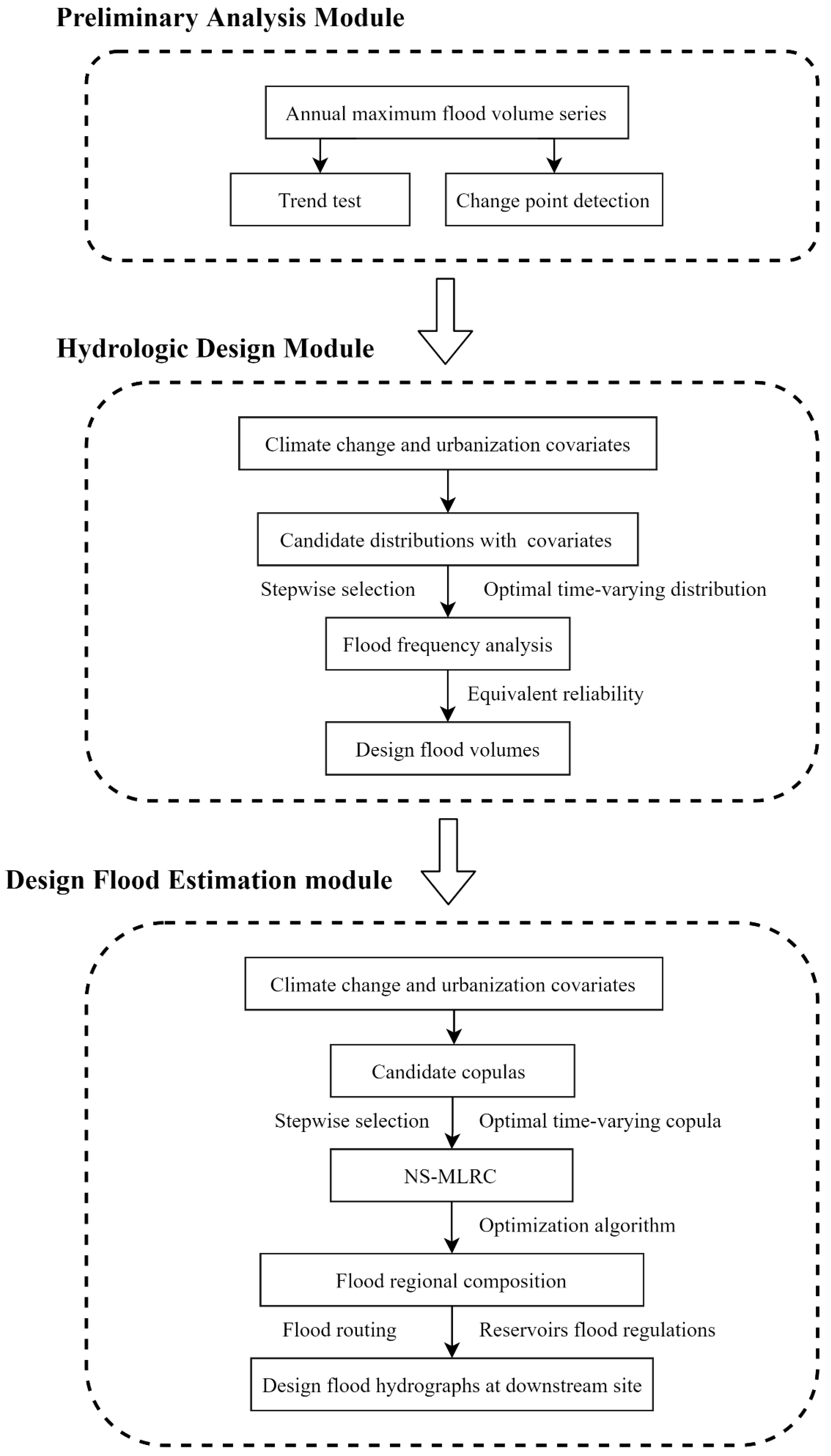
The flowchart of nonstationary design flood estimation for cascade reservoirs is shown in Figure 1, of which there are three main modules. The first module preliminarily analyzes the nonstationarity of the flood volume series. The second module calculates the design flood volumes based on nonstationary flood frequency analysis and ER criteria. The last module solves the flood regional compositions using the NS-MLRC method and derives the design flood hydrograph regulated by cascade reservoirs.
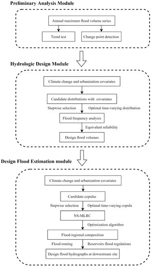
Figure 1.
Flowchart of nonstationary design flood estimation in response to climate change, population growth and cascade reservoir regulation.
2.1. Preliminary Analysis Module
This module aims to manipulate the dataset, determine the candidate univariate and multivariate distributions and covariates, and analyze the nonstationarity preliminarily.
2.1.1. Candidate Distribution Functions, Copulas and Covariates
For nonstationary univariate frequency analysis, the type of the probability distribution determines which form of frequency curves will be generated. Table 1 lists five probability distributions, namely Gamma, Weibull, Log-normal, Gumbel, and Pearson type III, which are the alternative distributions for flood frequency analysis with the different link functions [41,42,43]. On the other hand, the Archimedean copulas are widely used in hydrological researches [8,33]. Three mono-parameter Archimedean copulas, i.e., Gumbel-Hougaard, Frank and Clayton copulas (Table 2) are selected as the candidate copulas for the time-varying dependence structure modelling.

Table 1.
The univariate distributions used to model the flood series in this study.
Table 2.
Three Archimedean copulas used for the time-varying dependence structure modelling in this study.
The multiple covariates (i.e., explanatory variables, predictors or addictive terms) indicating both population growth and climate change are incorporated to explain the variation in nonstationary time series. The impact of urbanization and water consumption on the hydrologic flood series is considered by the population (Pop) [37,43], while the annual total precipitation (Prcp), one of the important hydro-climate factors, is applied to quantify the effects of climate change [10,44].
2.1.2. Trend Test and Change Point Detection
The Mann–Kendall trend test [45,46,47] and Pettitt’s test [48] are widely used for trend test and change point detection, which can be applied to analyze the nonstationarity of time series [43,44]. A nonparametric multiple change point analysis approach designed by Matteson and James [49] is used for change point analysis of multivariate time series in this study.
2.2. Hydrologic Design Module
This module is responsible for nonstationary flood frequency analysis and design flood volume estimation.
2.2.1. Time-Varying Moments
Generally, the nonstationary flood frequency analysis can be established by the time-varying moments [50,51] based on the GAMLSS model [27]. Furthermore, the time-varying moments can be improved by replacing time with other physical covariates which have physical meanings [8,10]. The generalized linear model (GLM) [52] is implemented to establish the function between distribution parameters and their predictors. To facilitate understanding, a three-parameter time-varying distribution is taken as an example in the remainder of this literature.
For the time-varying probability distribution function , let be the response variable at time () and the vector be the three time-varying parameters. Then each parameter can be expressed as a function of the covariates () via a link function as follows:
where are the link functions of distribution parameters for restricting the sample space [8]; are the GLM parameters. The time-varying moments are fitted by maximum penalized likelihood estimation [27,53]. The centile curve [54] and worm plot [55] are used for the goodness-of-fit test of univariate nonstationary distributions.
2.2.2. Selection of Time-Varying Distributions
The selection of the covariates and the type of probability distribution are the two steps for seeking the best time-varying moment model. For one specific time-varying distribution, the selection of covariates contains two aspects:
(1) The selection of the best GLM for a single parameter, which is conducted by the forward procedure [27]. In the forward procedure, all variables not currently in the model are considered for addition at each step, while all variables currently in the model are individually considered for deletion.
(2) For a given distribution, there exist diverse strategies to select the GLMs used to model all the parameters, i.e., μ, σ, and ν. The strategy proposed by Stasinopoulos and Rigby [27] is executed for GLMs selection of all the distribution parameters.
Since the shape parameter ν is too sensitive to the data series, it is often assumed as constant as other studies have done [10,56]. In practice, only the first two moments (i.e., μ and σ) are taken to consider nonstationary data series. The optimal probability distribution is selected from these five distributions mentioned in Table 1 based upon the Bayesian information criterion (BIC) [57]:
where ML denotes the log-likelihood within a likelihood-based inferential procedure; df represents the total effective degrees of freedom and; n is the length of the data series. Comparing with the widely used Akaike information criterion (AIC) [58], the BIC has a larger penalty on the over-fitting phenomenon.
After the above selection procedures is performed for each probability distribution, then the distribution corresponding to the smallest BIC value is selected as the optimal univariate distribution.
2.2.3. Equivalent Reliability (ER)
The hydrologic design criteria according to the definition of return period under stationary conditions might be modified to adapt nonstationarity [43,59]. To ensure that the nonstationary flood frequency analysis is closely relevant to the practical condition, the flood events can be linked with the design lifespan of hydraulic projects [39]. The project reliability in the no flood event exceeds the specific design value during the life period of the project, which is defined as follows [59]:
where is the exceedance probability at year for design value ; the superscript S and NS represent stationary and nonstationary conditions, respectively.
If a project is designed to withstand a flood event that occurs once in m years under stationary conditions, then the reliability within the design life period of the project is given by
The ER supposes that the hydrological design values derived using stationary and nonstationary flood control design standard should have the same reliability during the life time of hydraulic structures [39]. Assuming that , the nonstationary design value for a specific return period m is denoted by , which is measured by the following equation:
For given design life period and return period m, the stationary ER criteria is calculated by Equation (4) firstly, and then the nonstationary design value corresponding to m can be obtained eventually by solving Equation (5).
2.3. Design Flood Estimation Module
This module is used to establish the time-varying copula and derive the nonstationary design flood hydrographs based on the NS-MLRC method.
2.3.1. Time-Varying Dependence Parameter of Copulas
Traditional joint hydrological frequency analysis assumes that the parameters of both marginal distributions and copula functions are constant. Nevertheless, either the individual series or the dependence structure between the multiple series might be also nonstationary under changing environments [8,38]. To consider such possibility, a general form of the joint distribution of multiple random variables at any time , is built. According to Sklar’s theorem [60], the joint PDF can be expressed in terms of its marginal distributions and the associated dependence function, i.e., the time-varying copula can be expressed as follows:
where denotes the cumulative distribution function (CDF) that defines the dependence structure of multiple variables; represents the CDF of copula function; represents the CDF of the hydrological random variables; () are the time-varying marginal distribution parameters; denotes the time-varying copula parameter; and are the marginal CDFs of the time-varying copula, which should range on [0,1].
Like the univariate distribution parameters expressed in Equation (1), the time-varying copula parameter can also be expressed as a GLM function of the covariates via a proper link function as follows:
where relies on the limits of (Table 2); are the GLM parameters. The copula-based GAMLSS with non-random sample selection is applied in this study so that the non-stationarities of marginal distributions can be considered [61,62]. The time-varying dependence parameter of copula is estimated by a penalized likelihood framework with integrated automatic multiple smoothing parameter selections [63]. It is hard to calculate the distance between the fitted and the empirical frequency so that the Probability Integral Transformation (PIT) is used for the goodness-of-fit test of time-varying copula [64,65]. The forward procedure is applied for the selection of based on GLM, while the BIC criteria is used to select the optimal copula function.
2.3.2. Nonstationary Most Likely Regional Composition (NS-MLRC) Method
The sketch of flood regional composition with cascade reservoirs is shown in Figure 2, in which the random variables , and represent the natural inflow of reservoirs , intermediate basins , and downstream site C with the corresponding values , and , respectively.
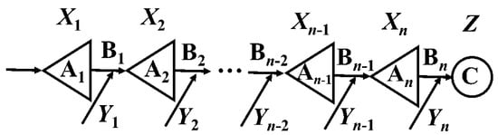
Figure 2.
Sketch diagram of the flood regional composition with cascade reservoirs.
For the A1-A2 sub-partition, the inflow of downstream reservoir A2(x2) consists of the inflow of reservoir A1(x1) and the inflow of intermediate basin B1(y1). The inflow of downstream reservoir A2 is affected by the operation of upstream reservoir A1. Then is determined as the FRC of , in which inflow can be turned into discharge based on the operation strategy of reservoir A1. Thus, the discharge of reservoir A2 is relevant to the FRC of A2, i.e.,. For the cascade reservoir system, all the FRC should satisfy the principle of the water balance equation [33]:
For the inherently stochastic mechanism of the flood generation, there exists multiple compositions of in compliance with the water balance equation. The output of the MLRC method is the FRC with the largest occurrence probability. Nevertheless, under changing environments, the FRC derived by the MLRC method may vary over time. According to Sklar’s theorem, the time-varying copula is expressed as follows
where denotes the PDF of copula; are the corresponding CDFs of , respectively; () and are the optimal time-varying marginal distributions of flood values occurring at reservoirs and downstream site C, respectively.
The composition is more likely to occur with the increase of PDF [66]. The NS-MLRC is obtained when is maximized by subjecting water balance constraint:
The joint PDF is maximized when its first-order derivative equals zero so that the following equation should be satisfied:
After deriving the composition from Equation (11), the NS-FRC can be obtained subsequently using NS-MLRC method. The Newton iteration algorithm is adopted to solve Equation (11) [33].
According to the flood prevention standard of cascade reservoirs, the design flood hydrographs of each sub-system are calculated by the peak and volume amplitude method [67,68] based on the results of the NS-MLRC method. River channel flood routing and reservoir flood control regulations are adopted to derive the design flood hydrograph at the downstream site C [34,69].
3. Study Area and Data
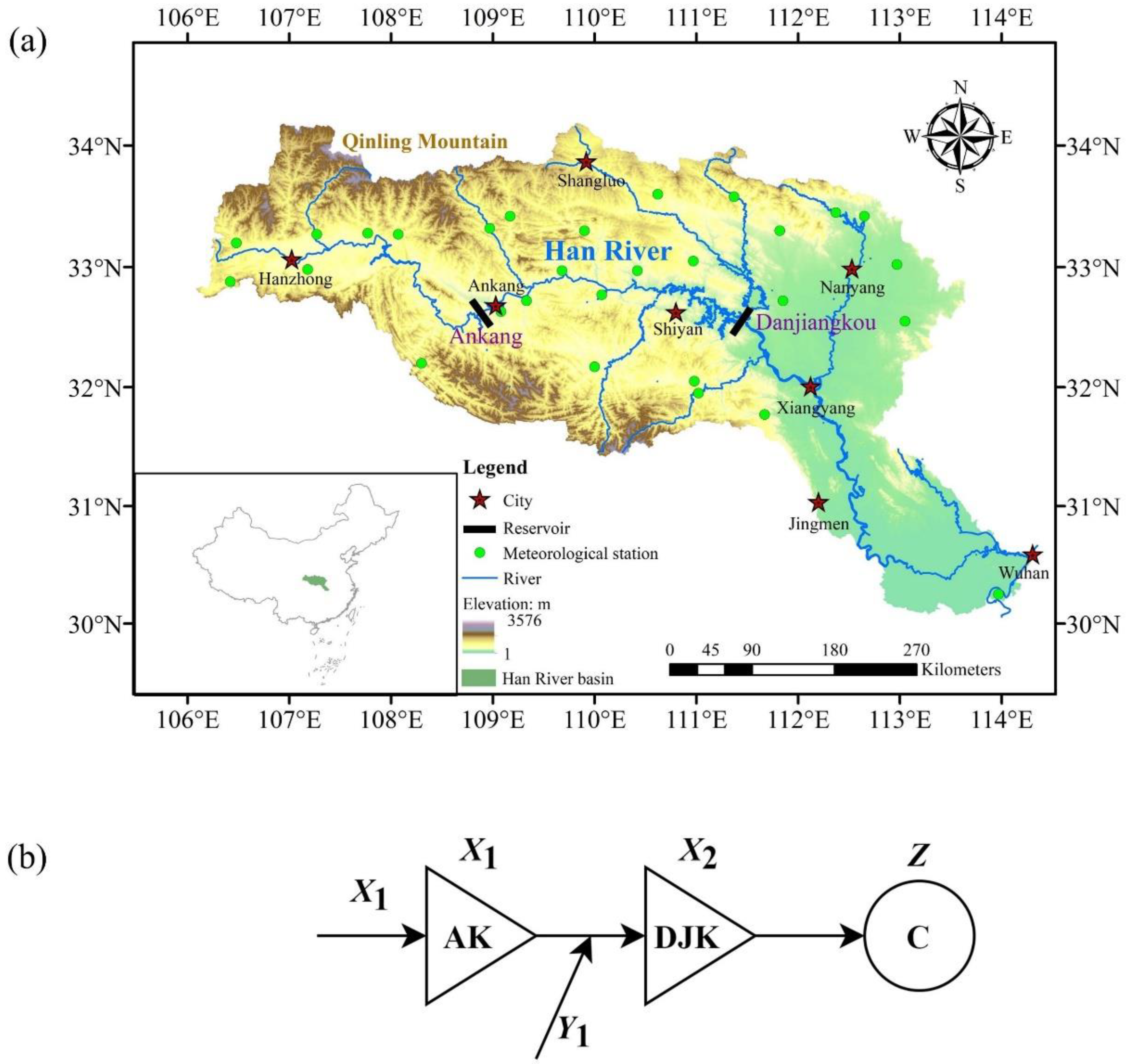
The Han River basin in China is located between 106–115° E and 30–35° N (see Figure 3), and has a total length of 1530 km. As one of the most important tributaries of the Yangtze River, The Han River rises in the southern of Qinling mountains, and flows from the northwest to the southeast. This mountainous region lies in the humid zone with a subtropical monsoonal climate. The annual average temperature is between 14 and 16 °C. The annual precipitation varies from 700 to 1100 mm, and about 70 to 80% of the annual precipitation occurs during the flood season (May to October), in which heavy rains in early summer and continuous rainfall in autumn often cause major floods.
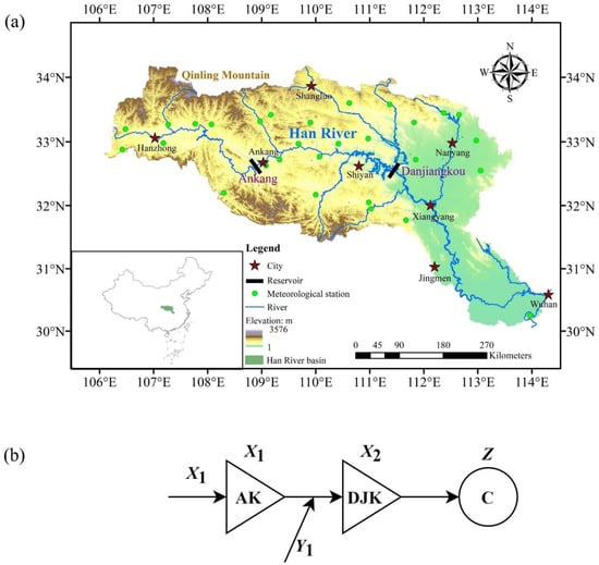
Figure 3.
(a) Map of the Han River basin and (b) sketch diagram of the flood regional composition with AK and DJK cascade reservoirs.
3.1. Cascade Reservoirs
The Ankang (AK) and Danjiangkou (DJK) cascade reservoirs are located at the upper and middle reach of the Han River basin, respectively. The AK reservoir was built in 1992 and provides hydropower generation and flood control, while the DJK reservoir was built in 1973 and its primary functions are flood control, water supply, hydropower generation, and irrigation. These two reservoirs are selected for the case study because their inflow data is lengthy enough (over 60 years) and they have large storage capacities.
The basic information of AK and DJK cascade reservoirs is listed in Table 3. The characteristic parameter values and current flood control operation rules of the AK and DJK reservoirs are provided by the Changjiang (Yangtze River) Water Resources Commission (CWRC), Ministry of Water Resource [70]. More information about AK and DJK reservoirs can be found in the references [71,72].
Table 3.
Characteristic parameter values of the cascade reservoirs in the Han River basin.
3.2. Dataset
Four categories of data series were collected, including restored streamflow data, observed hydro-climate data, population growth data and GCMs outputs from CMIP5. The observed data series provide information up to 2020, while a projected dataset of the future period from 2021 to 2095 is also used in this study.
(1) Restored mean daily streamflow data from both the inflow of AK reservoir and the inflow of DJK reservoir were provided by the Hydrology Bureau of the Changjiang (Yangtze River) Water Resources Commission during 1954–2020. The restoration of streamflow data can be taken as a natural flow series that eliminates the regulation impact of reservoirs.
(2) Observed daily precipitation series from 27 stations during 1951–2020 were obtained from the National Climate Center of the China Meteorological Administration (source: http://data.cma.cn/ (accessed on 16 April 2021)).
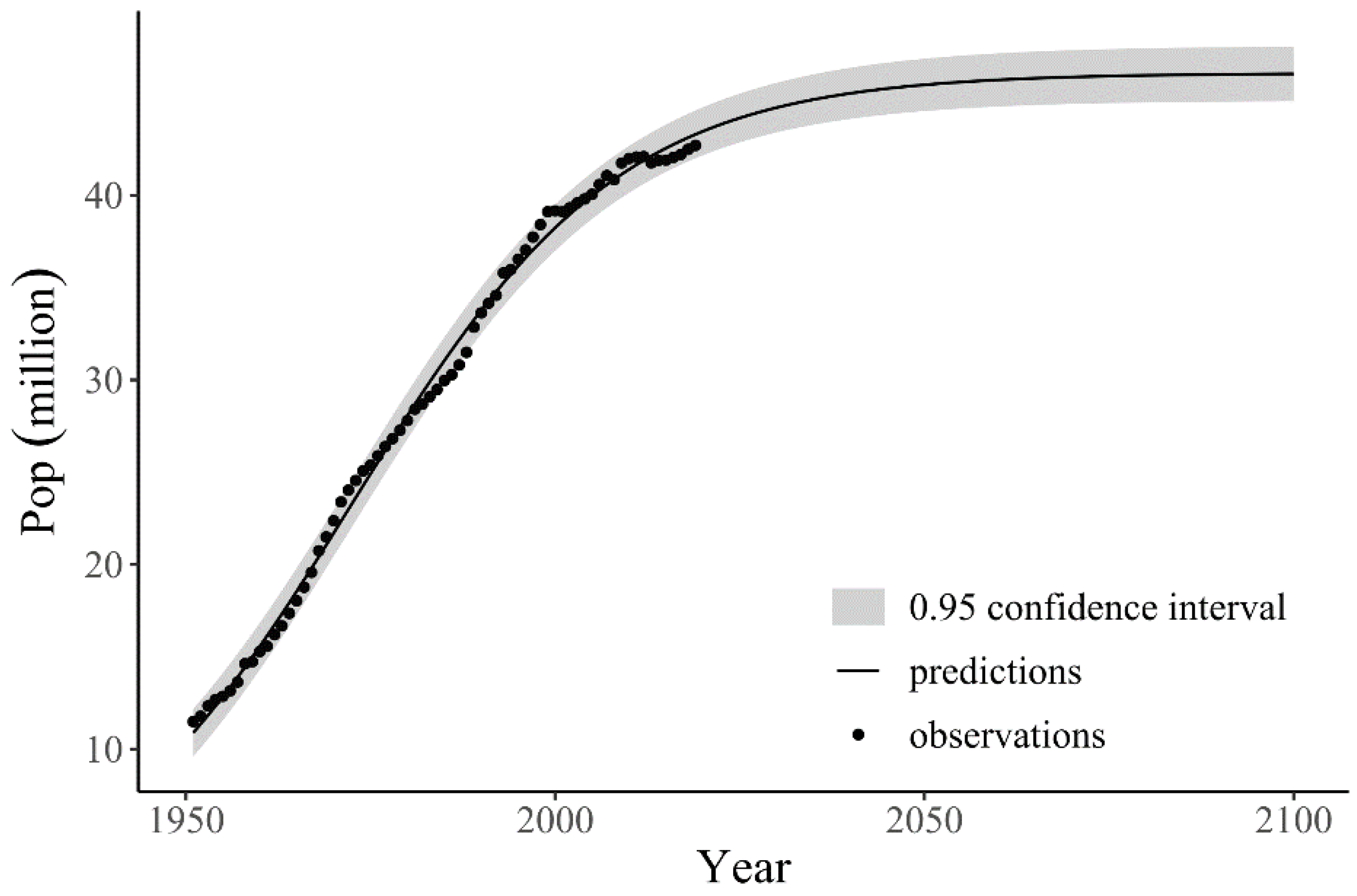
(3) Given the unavailability of population data at the basin scale, the total registered population of all the prefecture-level cities amidst in the Han River basin was collected. These cities include Wuhan, Shiyan, Jingmen, Xiangyang in Hubei province, Hanzhong, Ankang and Shangluo in Shanxi province, and Nanyang in Henan province. The annual registered population data in Han River basin were obtained from the China Compendium of Statistics 1949–2008 [73], the website of the National Bureau of Statistics of China (source: http://www.stats.gov.cn/tjsj/ndsj/ (accessed on 1 July 2021)) and the websites of statistical bureaus of the provinces and cities mentioned above. For future projection, the logistic growth model that adapts the growth restriction resulting from limited natural resources is applied to predict the growth of population [74]. Based on the logistic growth model, the evolution of the population for the period 1950–2100 is illustrated in Figure 4.
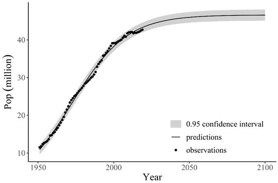
Figure 4.
Evolution of the population in Han River basin during 1950–2100.
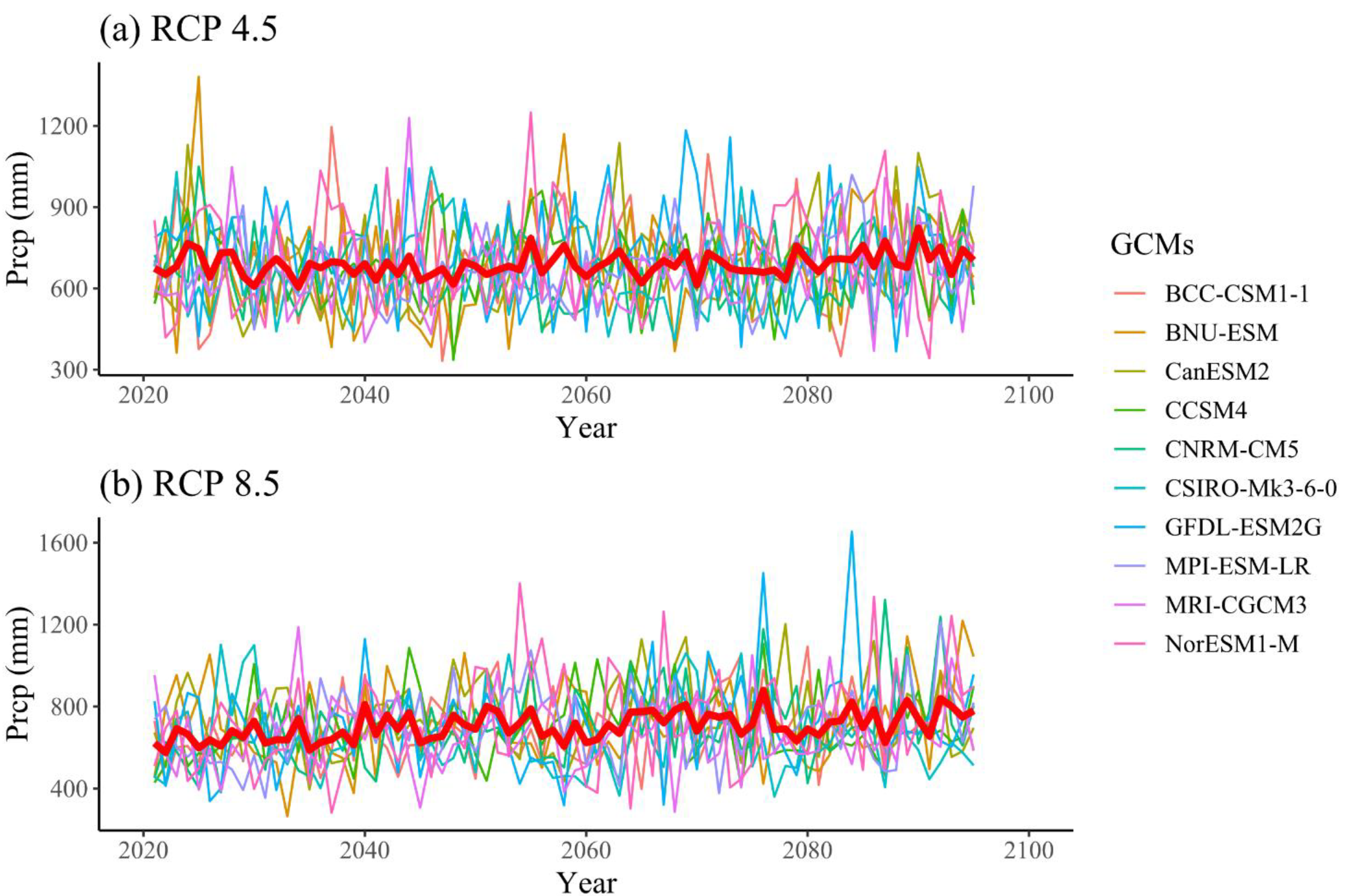
(4) Future daily precipitation is simulated by GCM using climate change scenarios [75]. Our lab research team, Tian et al. (2021) used 10 different GCMs (see Table 4) and two representative concentration pathways (RCPs) of 4.5 and 8.5 from the IPCC Fifth Assessment to project climate change for the Han River basin, which are employed in this study [76,77,78]. The RCP 4.5 scenario represents a future of medium emission where climate policies limit [79]. Without climate change policies, RCP 8.5 scenario presumes that high emissions of greenhouse gases continue in the future.
Table 4.
Description of the 10 GCMs used in this study.
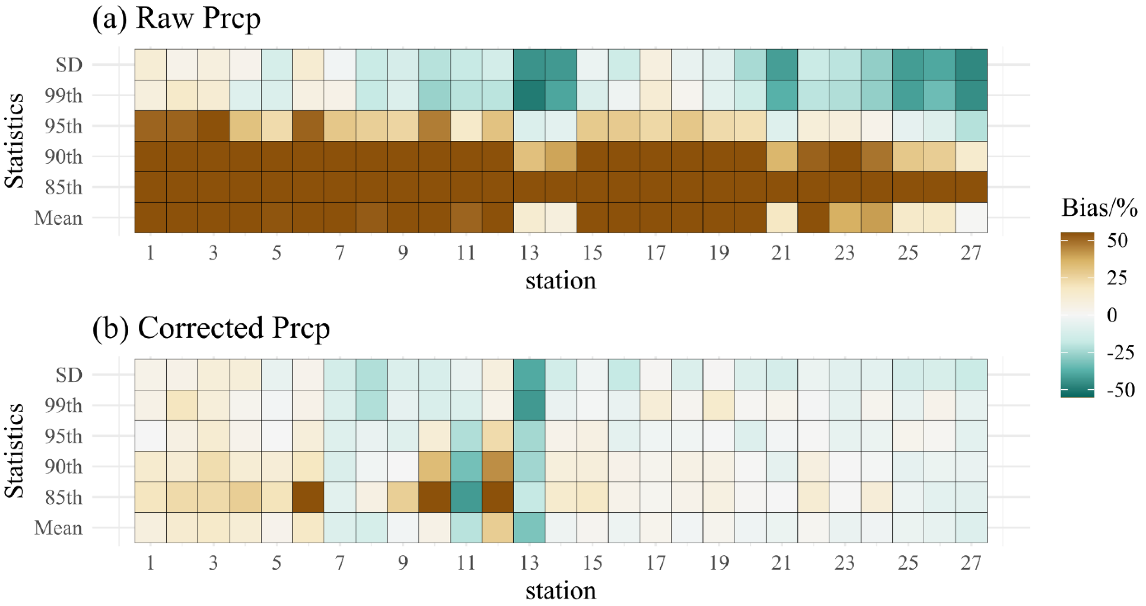
The outputs of the GCMs not only involve the historical period before 2006 as a reference, but also cover 2021–2095 for future projection. A daily bias correction method is applied in this study for statistical downscaling [80]. Six statistics containing mean, standard deviation, 85th, 90th, 95th and 99th percentiles of future precipitation series are used to test the performance of the daily bias correction method [80]. Taking the BCC-CSM1-1 model as an example, the bias of raw and the corrected model for daily precipitation series during 1991–2005 are illustrated in Figure 5, where the horizontal and vertical coordinates follow the 27 meteorological stations and the bias about the six statistics, respectively. These findings indicate the great performance of the statistical downscaling method so that it can be employed for future projection. Figure 6 shows the projected future precipitation under RCP 4.5 and RCP 8.5 scenarios. The arithmetic mean values of the 10 GCMs are employed in this study for nonstationary flood frequency analysis.
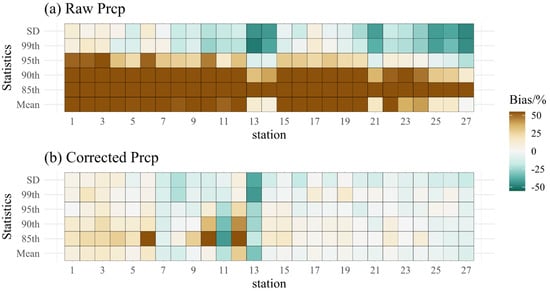
Figure 5.
The bias of (a) raw and (b) corrected BCC-CSM1-1 outputs during 1991–2005.

Figure 6.
Projected annual precipitation under (a) RCP 4.5 and (b) RCP 8.5 scenarios for 2021–2095. The bold red lines are the arithmetic mean value of the 10 GCMs.
4. Result Analysis
4.1. Preliminary Analysis
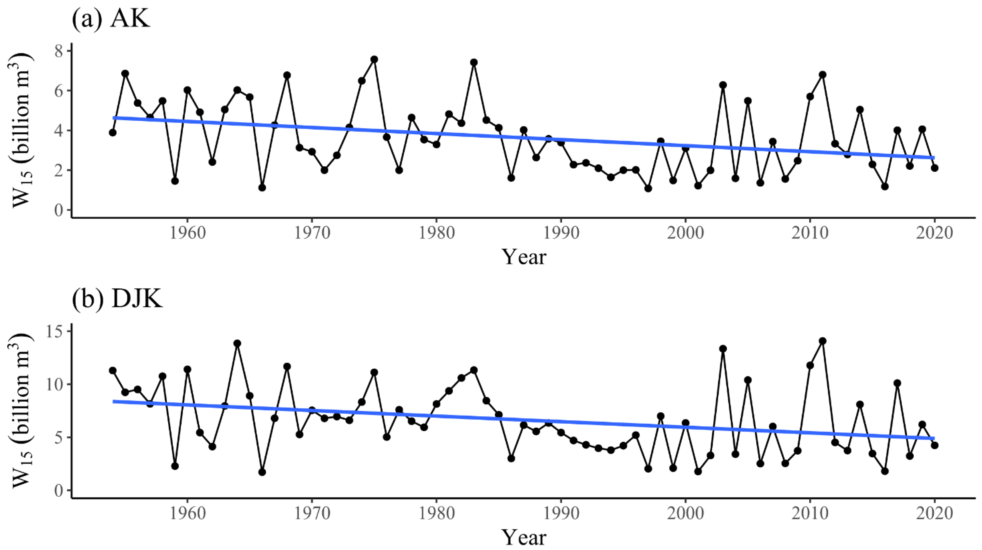
According to the regulation characteristics of cascade reservoirs in the Han River basin, the annual maximum 15-day (denoted as W15) flood volume series of the AK and DJK reservoir are selected for flood frequency analysis. Indicated by the fitted trend lines, the overall decreasing trends of W15 series in both AK and DJK reservoirs are shown in Figure 7. The significance of trends in the flood volume series and explanatory variables (i.e., Pop and Prcp) during 1954–2020 is analyzed by the Mann–Kendall test, and the Pettitt’s test is employed to detect the change points in the W15 series, which is summarized in Table 5. Findings show decreasing trends of the W15 series in both the AK and DJK reservoirs and the detected change-points are located at 1985–1986 (p-value < 0.05) for two reservoirs. The nonparametric multiple change point analysis method detects the change point of the W15 series between AK and DJK reservoirs, which takes place in 1985 (p-value < 0.05). This preliminary analysis demonstrates that both the univariate series and the dependence structure between the W15 series are all nonstationary.
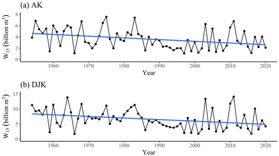
Figure 7.
The W15 series with the fitted linear trend lines of (a) AK and (b) DJK reservoirs.
Table 5.
Results of trend test, change-point detection and multiple change point analysis for the W15 series for the years 1954–2020 (* means the maximum of the absolute value of the vector U).
4.2. Nonstationary Design Flood Volumes
4.2.1. Univariate Nonstationary Flood Frequency Analysis
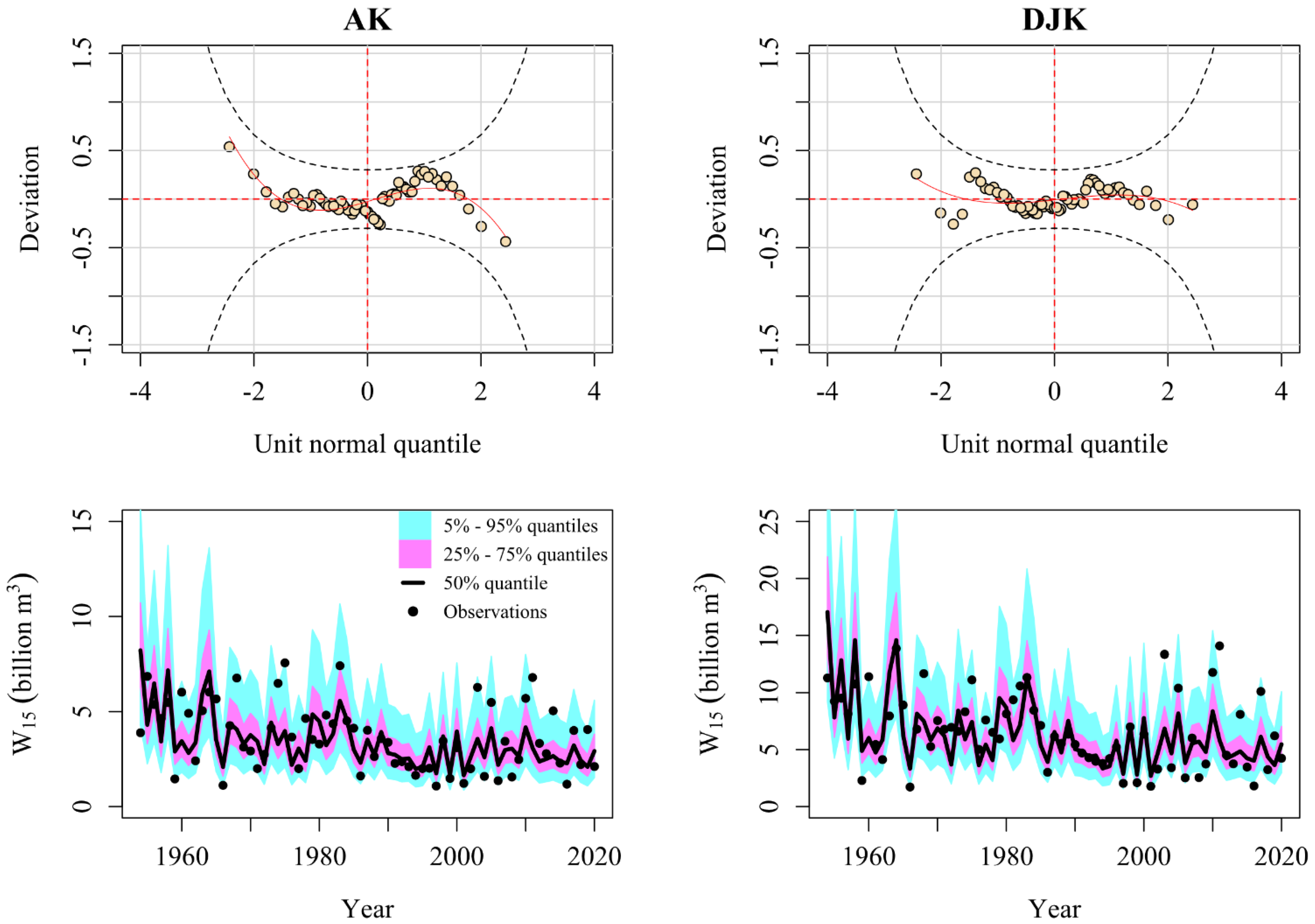
Based on the selection procedure mentioned in Section 2.2.2, we assume that the lower bounds of forward stepwise procedure for both μ and σ are constant (i.e., μ ~1, σ ~1), while the upper bounds are (Pop + Prcp). Table 6 lists the distribution parameters and BIC values for W15 at the AK and DJK reservoirs, in which the time-varying BICNS and constant BICS are also calculated. According to the minimum BICNS values, the Log-normal distribution is the best one for the W15 series in both the AK and DJK reservoirs. To demonstrate the fitting process, the detailed forward procedure applied in Log-normal distribution parameter μ is displayed in Table 7. The worm plot and centile curves for the Log-normal distribution are plotted in Figure 8. In the worm plot, all scatter points are within the 95% confidence intervals, illustrating a good fit between the optimal distribution and empirical frequency series. In terms of centile curves, the percentages of observation points within the 5th, 25th, 50th, 75th and 95th intervals are 5.97%, 26.86%, 59.70%, 70.14% and 94.02% (5.97%, 28.35%, 53.73%, 71.64% and 94.02%) for AK (DJK), respectively. The above results indicate that the selected optimal Log-normal distribution is more adequate to model the nonstationarity of the W15 series, and to express the similar type of GLMs for both AK and DJK reservoirs. As presented in Table 6, the location parameter of Log-normal distribution for modelling the W15 series is linked to Prcp and Pop while the scale parameter of W15 is constant. Furthermore, the BICNS value is always smaller than the BICS value for the same distribution. Compared to the stationary distributions, the optimal nonstationary Log-normal distribution can satisfactorily capture the nonstationarity in flood frequency analysis for both the AK and DJK reservoirs.
Table 6.
Distribution parameters and BIC values for W15 at the AK and DJK reservoirs.
Table 7.
The detailed forward procedure of Log-normal distribution for W15 at the DJK reservoir.
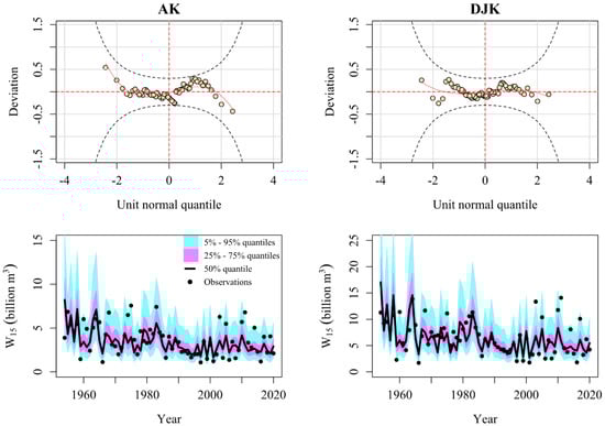
Figure 8.
Diagnostic plots (worm plot and centile curves) for evaluating the goodness-of-fit of the optimal nonstationary Log-normal distribution for the W15 series in the AK and DJK reservoirs.
4.2.2. Design Flood Volumes in DJK Reservoir
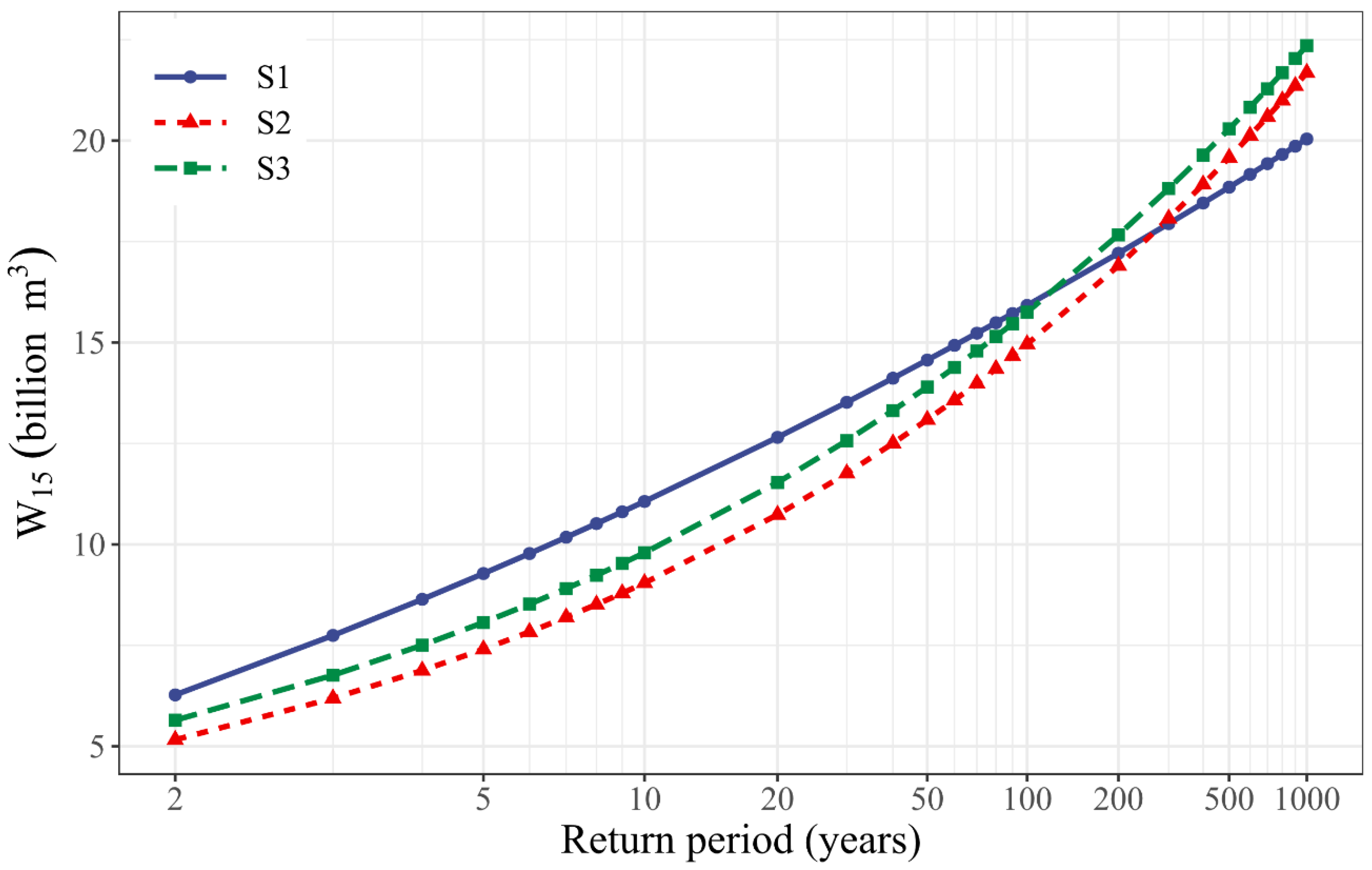
The nonstationary design value is essential for handling changing environments in considering future flood risk management. Since the total storage capacity of the DJK reservoir is approximately 31 times larger than that of the AK reservoir (Table 3), the DJK reservoir is considered as the key flood prevention project in the Han River basin. If we assume that the design lifespan for the DJK reservoir is 100 years (from 1973 to 2072), then the years of 2021–2072 are chosen as future projections. The design flood volume under nonstationary conditions is calculated by the ER criteria. Three scenarios, i.e., stationary distribution condition (S1), nonstationary conditions based on RCP 4.5 (S2), or RCP 8.5 (S3), are compared. It is worth noting that the S1 scenario only takes cascade reservoir regulation into account while the nonstationary attributes of climate change and population growth are omitted. To produce an intuitive comparison among these scenarios, Figure 9 plots the stationary and nonstationary design flood volumes W15 for return period . It should be noted that the design flood volumes in the stationary reference scenario are estimated by the Pearson type III distribution and curve-fitting estimation method recommended by the Ministry of Water Resources in China [32]. It is found that the design flood volumes of S2 (S3) are lower than S1 when the return periods are less than 300 (200) years, respectively. The design flood volumes of S3 are always larger than S2. Compared with the nonstationary distribution scenarios (i.e., S2 and S3), the method used under the S1 scenario overestimates the flood volumes at a lower return period while the extreme event is underestimated at a higher return period. For the 1000-year return period, the design W15 in the DJK reservoir under S1, S2 and S3 scenarios are 20.041, 21.680 and 22.352 billion m3, respectively. These results indicate that climate change and population growth have greater impact on the features of future W15 under the S2 and S3 scenarios so that the large uncertainty and flood hazard should be considered for future hydrological design and water resources management.
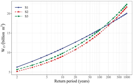
Figure 9.
Comparison of design W15 with different return periods and scenarios for the DJK reservoir.
4.3. Design Flood Estimation at Downstream Site
4.3.1. Nonstationary Flood Regional Composition
After the estimation of the design flood volumes at the DJK reservoir, the flood regional composition method can be applied for analyzing the flood generation mechanism of the cascade reservoirs in the Han River basin. For nonstationary analysis of the dependence structure, the forward selection procedure is implemented to model the dependence parameter of three copulas, i.e., the Gumbel-Hougaard, Frank, and Clayton copula. The lower and upper bounds of forward stepwise procedure for θc are constant (i.e., θc ~1) and (Pop + Prcp), respectively. Table 8 summarizes the fitted dependence parameters and the goodness-of-fit results for the optimal copulas under three scenarios for nonstationary modeling of the W15 series in AK and DJK reservoirs. The p-KS(Z1) and p-KS(Z2) are p-values of the KS test for the two Rosenblatt’s probabilities integral transformations Z1 and Z2, which should be uniformly and independently distributed on [0,1]. The p-Kendall is the p-value of the Kendall rank correlation test for Z1 and Z2. Table 8 shows that the p-KS(Z1), p-KS(Z2) and the p-Kendall values are larger than 0.05, which statistically supports the validity of the hypothetical models. The time-varying Gumbel-Hougaard copula is the optimal copula to model the dependence structure of the W15 series by comparing the BIC values. Obviously, the nonstationary spatial correlation of flood events can be sufficiently explained by the NS-MLRC method.
Table 8.
Dependence parameters and goodness-of-fit results for candidate copulas in nonstationary modeling.
Figure 3b illustrates that the flood volumes of the DJK reservoir are decomposed to the outflow of the AK reservoir and the inflow of the AK-DJK inter-basin. It is noted that the return period of the design flood is 1000 years in both the AK and DJK reservoirs, as shown in Table 3. The Log-normal distributions with explanatory variables shown in Table 6 are applied as the marginal distributions of the time-varying copulas. Following the procedures described in Section 2.3.2, the NS-MLRC results of the cascade reservoirs can be estimated.
Based on the NS-MLRC method, the nonstationary FRC of the AK and DJK reservoirs with the maximum occurrence probabilities are derived. It should be noted that there are one hundred (from 1973 to 2072) FRCs derived by the NS-MLRC method, compared with the individual result calculated by the MLRC method. Table 9 compares the FRC results under three scenarios during design lifespan with the same flood prevention standard according to ER. It is shown that the designed W15 in the AK reservoir (X1) of S2 and S3 is greater than that of nonstationary cases, while the design W15 at the (Y1) are overestimated when compared with S1.
Table 9.
The FRC results derived by the MLRC (S1 scenario) and NS-MLRC (S2 and S3 scenarios) methods during design lifespan with the same flood prevention standards based on ER. X1, Y1 and X2 represent the designed flood volume W15 at the AK reservoir, inter-basin, and the DJK reservoir, respectively.
4.3.2. Design Flood Hydrographs at Downstream Site
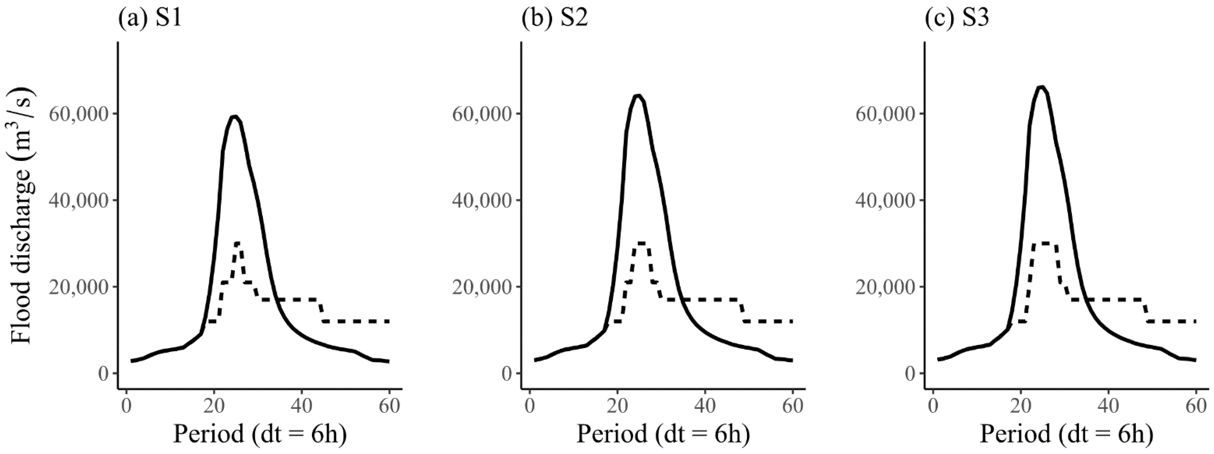
The estimation of design floods at downstream sites can be obtained using design inflow hydrographs and cascade reservoir regulations based on the derived FRC results. Different FRCs may differ in terms of their occurrence probabilities [35], and the FRCs with maximum occurrence probabilities among the lifespan of projects are analyzed. To generate the design flood at the downstream site C (Figure 3), the current flood control regulation and the commonly used Muskingum model provided by the CWRC are used. After flood control operation, 1000-year design flood hydrographs for the downstream sites under three scenarios with or without reservoir regulation are plotted in Figure 10. Table 10 lists the results of the 1000-year design floods under three scenarios with or without reservoir regulation.
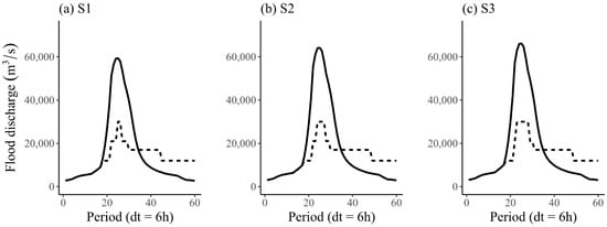
Figure 10.
Design flood hydrographs of 1000-year return period at downstream under three scenarios with (dash line) or without (solid line) cascade reservoir regulation.
Table 10.
Comparison of 1000-year design floods under three scenarios with or without reservoir regulation.
Figure 10 shows that the 1000-year design flood hydrographs vary considerably with less peaks and gentler flood processes at downstream sites after cascade reservoir regulation. As shown in Table 10, the design floods of the cascade reservoirs decrease significantly on account of the regulation of the AK and DJK reservoirs. Taking Qmax as an example, under the S1, S2, and S3 scenarios, the 1000-year design Qmax of AK (DJK) at downstream sites decreased by 10.97% (49.43%), 5.06% (53.25%) and 5.31% (54.66%), respectively due to cascade reservoir regulation. Furthermore, the W1 and W3 flood volumes are less than half of these without cascade reservoir regulation.
5. Discussion
5.1. Nonstationary Characteristics
Flood events differ according to climate, reservoir regulation, water consumption, and land use, which are the potential driving forces that link to flood design. When traditional hydrologic design criteria are extended for accommodating nonstationary conditions, the future covariates should be obtained on account of the hydraulic lifespan. However, it is difficult to predict the changes of some variables, such as deforestation, so that other land use indices are not considered in this study. Based on the case study in the Han River, the influence of climate change, population growth and cascade reservoir regulation on the design flood at the downstream site are discussed as follows.
Many studies have identified how the changing pattern brings diverse control on a flow process [28,33], which can be classified as either a direct and/or indirect impact. Climate change and population growth will alter the regional hydrological characteristics of the basin, and affect the flood data series as well as the flood design (Figure 8) [43]. Compared to these prolonged effects, the cascade reservoir regulation clips the flood peak and decreases the flood volumes in a transitory and swift way (Figure 10). Among the multiple driving patterns, the cascade reservoir regulation plays a dominant role in affecting the design floods at downstream sites. Furthermore, the cascade reservoir flood control strategies can be re-regulated for adapting the slow-to-change non-stationarity (such as climate change and population growth) in future work.
5.2. The Worst FRC during Reservoir Lifespan
In practical operations, the worst FRC during reservoir lifespan is more noteworthy in comparison with the most likely FRC. The reservoir water level is at the flood limited water level during flood season to provide sufficient storage for possible floods [81]. When a flood event occurs, the highest water level during the period of reservoir flood regulation can quantificationally indicate the flood hazard, such as dam-break risk, downstream inundation risk and so on. In this study, the highest water level of the DJK reservoir during the whole flood regulation process is applied as an indicator to specifically represent the hazard of flood events.
Although the MLRC method has a strong statistical basis and generates a single regional composition, it is unable to evaluate the composition of the worst regional flood. The NS-MLRC method can include varying factors such as precipitation and population growth. In this study, variant FRCs derived by the NS-MLRC method are used to amplify the typical flood hydrograph, forming one hundred (from 1973 to 2072) FRC types. After cascade reservoir regulation, the comparison of the highest water levels derived from both the most likely FRCs and the worst FRCs at the DJK reservoir during its lifespan is demonstrated in Table 11. It indicates that the highest water level estimated by the most likely FRC is lower than that of the worst FRC, which means the worst FRC under the S2 and S3 scenarios is more adverse than the most likely FRC. In practice, the worst FRC in S3 is worthy of noting for future flood risk management.
Table 11.
Comparison of the highest water level derived from both the most likely FRC and the worst FRC during reservoir lifespan at the DJK reservoir for different scenarios.
6. Conclusions
There is an increasing need to develop an effective design flood estimation framework to deal with nonstationary data series caused by climate change and anthropogenic activities. In this study, the univariate flood frequency analysis, nonstationary hydrologic design criteria and the NS-MLRC method were adopted to derive the nonstationary design flood volumes in the Han River. The design flood hydrographs at the downstream site were estimated after cascade reservoir regulation. The main conclusions are summarized as follows:
(1) The proposed NS-MLRC method can be effectively implemented as an extension of the MLRC method for explaining the nonstationary spatial correlation of the flood events. The multiple nonstationary driving forces, i.e., climate change and population growth, can be captured and precisely quantified by the proposed design flood estimation framework.
(2) The slow-to-change impacts of climate change and population growth are presented in design flood volumes according to the nonstationary flood frequency analysis method and ER criteria. The long-lasting driving factors imply the larger risks of the flood hazard. The 1000-year design W15 of the DJK reservoir under the stationary distribution scenario (S1), RCP 4.5-based (S2), and the RCP 8.5-based (S3) nonstationary scenario are 20.041, 21.680 and 22.352 billion m3, respectively.
(3) The swift effects of cascade reservoirs are reflected in design flood hydrographs with lower peaks and less volumes based on the NS-MLRC method and flood control operation rules. For instance, the 1000-year design Qmax of the AK (DJK) downstream site under the stationary distribution scenario (S1), RCP 4.5-based (S2), and RCP 8.5-based (S3) nonstationary scenario decrease by 10.97% (49.43%), 5.06% (53.25%) and 5.31% (54.66%), respectively due to cascade reservoir regulation.
As the dominant element affecting flood design, the current cascade reservoir operation strategies can be improved to accommodate the slow-to-change nonstationarity in further research.
Author Contributions
Y.X.: Conceptualization, Data curation, Methodology, Visualization. S.G., L.X.: Methodology, Supervision. J.T.: Resources, Data Curation. F.X.: Methodology, Validation. All authors have read and agreed to the published version of the manuscript.
Funding
This study was financially supported by the National Natural Science Foundation of China (51879192), China Three Gorges Corporation (0799254), and the Research Council of Norway (FRINATEK Project No. 274310).
Data Availability Statement
Data sharing is not applicable to this article as no new data were created or analyzed in this study.
Acknowledgments
The numerical calculations in this paper have been done on the supercomputing system in the Supercomputing Center of Wuhan University.
Conflicts of Interest
The authors declare no competing interests. The corresponding author is responsible for submitting a competing interest statement on behalf of all authors of the paper.
References
- Milly, P.C.D.; Betancourt, J.; Falkenmark, M.; Hirsch, R.M.; Kundzewicz, Z.W.; Lettenmaier, D.P.; Stouffer, R.J. Stationarity Is Dead: Whither Water Management? Science 2008, 319, 573–574. [Google Scholar] [CrossRef]
- Benyahya, L.; Gachon, P.; St-Hilaire, A.; Laprise, R. Frequency Analysis of Seasonal Extreme Precipitation in Southern Quebec (Canada): An Evaluation of Regional Climate Model Simulation with Respect to Two Gridded Datasets. Hydrol. Res. 2013, 45, 115–133. [Google Scholar] [CrossRef]
- Onyutha, C.; Willems, P. Uncertainty in Calibrating Generalised Pareto Distribution to Rainfall Extremes in Lake Victoria Basin. Hydrol. Res. 2014, 46, 356–376. [Google Scholar] [CrossRef]
- Qu, C.; Li, J.; Yan, L.; Yan, P.; Cheng, F.; Lu, D. Non-Stationary Flood Frequency Analysis Using Cubic B-Spline-Based Gamlss Model. Water 2020, 12, 1867. [Google Scholar] [CrossRef]
- Zhang, T.; Su, X.; Feng, K. The Development of a Novel Nonstationary Meteorological and Hydrological Drought Index Using the Climatic and Anthropogenic Indices as Covariates. Sci. Total Environ. 2021, 786, 147385. [Google Scholar] [CrossRef]
- Javelle, P.; Ouarda, T.B.M.J.; Lang, M.; Bobée, B.; Galéa, G.; Grésillon, J.-M. Development of Regional Flood-Duration–Frequency Curves Based on the Index-Flood Method. J. Hydrol. 2002, 258, 249–259. [Google Scholar] [CrossRef]
- Brandimarte, L.; Di Baldassarre, G. Uncertainty in Design Flood Profiles Derived by Hydraulic Modelling. Hydrol. Res. 2012, 43, 753–761. [Google Scholar] [CrossRef] [Green Version]
- Jiang, C.; Xiong, L.; Xu, C.-Y.; Guo, S. Bivariate Frequency Analysis of Nonstationary Low-Flow Series Based on the Time-Varying Copula. Hydrol. Process. 2015, 29, 1521–1534. [Google Scholar] [CrossRef]
- López, J.; Francés, F. Non-Stationary Flood Frequency Analysis in Continental Spanish Rivers, Using Climate and Reservoir Indices as External Covariates. Hydrol. Earth Syst. Sci. 2013, 17, 3189–3203. [Google Scholar] [CrossRef] [Green Version]
- Yan, L.; Li, L.; Yan, P.; He, H.; Li, J.; Lu, D. Nonstationary Flood Hazard Analysis in Response to Climate Change and Population Growth. Water 2019, 11, 1811. [Google Scholar] [CrossRef] [Green Version]
- Debele, S.E.; Bogdanowicz, E.; Strupczewski, W.G. Around and about an Application of the GAMLSS Package to Non-Stationary Flood Frequency Analysis. Acta Geophys. 2017, 65, 885–892. [Google Scholar] [CrossRef] [Green Version]
- Hui, R.; Herman, J.; Lund, J.; Madani, K. Adaptive Water Infrastructure Planning for Nonstationary Hydrology. Adv. Water Resour. 2018, 118, 83–94. [Google Scholar] [CrossRef]
- Villarini, G.; Smith, J.A.; Serinaldi, F.; Bales, J.; Bates, P.D.; Krajewski, W.F. Flood Frequency Analysis for Nonstationary Annual Peak Records in an Urban Drainage Basin. Adv. Water Resour. 2009, 32, 1255–1266. [Google Scholar] [CrossRef]
- Salvadore, E.; Bronders, J.; Batelaan, O. Hydrological Modelling of Urbanized Catchments: A Review and Future Directions. J. Hydrol. 2015, 529, 62–81. [Google Scholar] [CrossRef]
- Wang, H.; Mei, C.; Liu, J.; Shao, W. A New Strategy for Integrated Urban Water Management in China: Sponge City. Sci. China Technol. Sci. 2018, 61, 317–329. [Google Scholar] [CrossRef]
- Sto Domingo, N.D.; Refsgaard, A.; Mark, O.; Paludan, B. Flood Analysis in Mixed-Urban Areas Reflecting Interactions with the Complete Water Cycle through Coupled Hydrologic-Hydraulic Modelling. Water Sci. Technol. J. Int. Assoc. Water Pollut. Res. 2010, 62, 1386–1392. [Google Scholar] [CrossRef]
- Xu, Y.; Xu, J.; Ding, J.; Chen, Y.; Yin, Y.; Zhang, X. Impacts of Urbanization on Hydrology in the Yangtze River Delta, China. Water Sci. Technol. J. Int. Assoc. Water Pollut. Res. 2010, 62, 1221–1229. [Google Scholar] [CrossRef] [Green Version]
- Zhao, G.; Gao, H.; Naz, B.S.; Kao, S.-C.; Voisin, N. Integrating a Reservoir Regulation Scheme into a Spatially Distributed Hydrological Model. Adv. Water Resour. 2016, 98, 16–31. [Google Scholar] [CrossRef] [Green Version]
- He, S.; Guo, S.; Chen, K.; Deng, L.; Liao, Z.; Xiong, F.; Yin, J. Optimal Impoundment Operation for Cascade Reservoirs Coupling Parallel Dynamic Programming with Importance Sampling and Successive Approximation. Adv. Water Resour. 2019, 131, 103375. [Google Scholar] [CrossRef]
- Zhang, Q.; Chen, Y.; Tao, X.; Xu, C.-Y.; Chen, X. A Spatial Assessment of Hydrologic Alteration Caused by Dam Construction in the Middle and Lower Yellow River, China. Hydrol. Process. 2008, 22, 3829–3843. [Google Scholar] [CrossRef]
- Wang, W.; Li, H.-Y.; Leung, L.R.; Yigzaw, W.; Zhao, J.; Lu, H.; Deng, Z.; Demisie, Y.; Blöschl, G. Nonlinear Filtering Effects of Reservoirs on Flood Frequency Curves at the Regional Scale. Water Resour. Res. 2017, 53, 8277–8292. [Google Scholar] [CrossRef]
- Strupczewski, W.G.; Singh, V.P.; Feluch, W. Non-Stationary Approach to at-Site Flood Frequency Modelling I. Maximum Likelihood Estimation. J. Hydrol. 2001, 248, 123–142. [Google Scholar] [CrossRef]
- Strupczewski, W.G.; Kaczmarek, Z. Non-Stationary Approach to at-Site Flood Frequency Modelling II. Weighted Least Squares Estimation. J. Hydrol. 2001, 248, 143–151. [Google Scholar] [CrossRef]
- Strupczewski, W.G.; Singh, V.P.; Mitosek, H.T. Non-Stationary Approach to at-Site Flood Frequency Modelling. III. Flood Analysis of Polish Rivers. J. Hydrol. 2001, 248, 152–167. [Google Scholar] [CrossRef]
- Zhang, Q.; Gu, X.; Singh, V.P.; Xiao, M.; Chen, X. Evaluation of Flood Frequency under Non-Stationarity Resulting from Climate Indices and Reservoir Indices in the East River Basin, China. J. Hydrol. 2015, 527, 565–575. [Google Scholar] [CrossRef]
- Wen, Q.; Sun, P.; Zhang, Q.; Li, H. Nonstationary Ecological Instream Flow and Relevant Causes in the Guai River Basin, China. Water 2021, 13, 484. [Google Scholar] [CrossRef]
- Stasinopoulos, D.M.; Rigby, R.A. Generalized Additive Models for Location Scale and Shape (GAMLSS) in r. J. Stat. Softw. 2007, 23. [Google Scholar] [CrossRef] [Green Version]
- Du, T.; Xiong, L.; Xu, C.-Y.; Gippel, C.J.; Guo, S.; Liu, P. Return Period and Risk Analysis of Nonstationary Low-Flow Series under Climate Change. J. Hydrol. 2015, 527, 234–250. [Google Scholar] [CrossRef] [Green Version]
- Mondal, A.; Mujumdar, P.P. Return Levels of Hydrologic Droughts under Climate Change. Adv. Water Resour. 2015, 75, 67–79. [Google Scholar] [CrossRef]
- Su, C.; Chen, X. Assessing the Effects of Reservoirs on Extreme Flows Using Nonstationary Flood Frequency Models with the Modified Reservoir Index as a Covariate. Adv. Water Resour. 2019, 124, 29–40. [Google Scholar] [CrossRef]
- Xiong, B.; Xiong, L.; Xia, J.; Xu, C.-Y.; Jiang, C.; Du, T. Assessing the Impacts of Reservoirs on Downstream Flood Frequency by Coupling the Effect of Scheduling-Related Multivariate Rainfall with an Indicator of Reservoir Effects. Hydrol. Earth Syst. Sci. 2019, 23, 4453–4470. [Google Scholar] [CrossRef] [Green Version]
- Ministry of Water Resources. Regulation for Calculating Design Flood of Water Resources and Hydropower Projects; China Water & Power Press: Beijing, China, 2006. [Google Scholar]
- Guo, S.; Muhammad, R.; Liu, Z.; Xiong, F.; Yin, J. Design Flood Estimation Methods for Cascade Reservoirs Based on Copulas. Water 2018, 10, 560. [Google Scholar] [CrossRef] [Green Version]
- Xiong, F.; Guo, S.; Yin, J.; Tian, J.; Rizwan, M. Comparative Study of Flood Regional Composition Methods for Design Flood Estimation in Cascade Reservoir System. J. Hydrol. 2020, 590, 125530. [Google Scholar] [CrossRef]
- Xiong, F.; Guo, S.; Liu, P.; Xu, C.-Y.; Zhong, Y.; Yin, J.; He, S. A General Framework of Design Flood Estimation for Cascade Reservoirs in Operation Period. J. Hydrol. 2019, 577, 124003. [Google Scholar] [CrossRef]
- Sarhadi, A.; Burn, D.H.; Concepción Ausín, M.; Wiper, M.P. Time-Varying Nonstationary Multivariate Risk Analysis Using a Dynamic Bayesian Copula. Water Resour. Res. 2016, 52, 2327–2349. [Google Scholar] [CrossRef]
- Jiang, C.; Xiong, L.; Yan, L.; Dong, J.; Xu, C.-Y. Multivariate Hydrologic Design Methods under Nonstationary Conditions and Application to Engineering Practice. Hydrol. Earth Syst. Sci. 2019, 23, 1683–1704. [Google Scholar] [CrossRef] [Green Version]
- Feng, Y.; Shi, P.; Qu, S.; Mou, S.; Chen, C.; Dong, F. Nonstationary Flood Coincidence Risk Analysis Using Time-Varying Copula Functions. Sci. Rep. 2020, 10, 3395. [Google Scholar] [CrossRef]
- Liang, Z.; Hu, Y.; Huang, H.; Wang, J.; Li, B. Study on the Estimation of Design Value under Non-Stationary Environment. South-North Water Transf. Water Sci. Technol. 2016, 14, 50–53. [Google Scholar] [CrossRef] [PubMed]
- Wang, J.; Li, B.; Wang, H. Concept of Equivalent Reliability for Estimating the Design Flood under Non-Stationary Conditions. Water Resour. Manag. 2018, 32, 997–1011. [Google Scholar] [CrossRef]
- Koutrouvelis, I.A.; Canavos, G.C. Estimation in the Pearson Type 3 Distribution. Water Resour. Res. 1999, 35, 2693–2704. [Google Scholar] [CrossRef]
- Villarini, G.; Serinaldi, F.; Smith, J.A.; Krajewski, W.F. On the Stationarity of Annual Flood Peaks in the Continental United States during the 20th Century: Stationarity of Annual Flood Peaks. Water Resour. Res. 2009, 45. [Google Scholar] [CrossRef]
- Yan, L.; Xiong, L.; Guo, S.; Xu, C.-Y.; Xia, J.; Du, T. Comparison of Four Nonstationary Hydrologic Design Methods for Changing Environment. J. Hydrol. 2017, 551, 132–150. [Google Scholar] [CrossRef]
- Xiong, B.; Xiong, L.; Chen, J.; Xu, C.-Y.; Li, L. Multiple Causes of Nonstationarity in the Weihe Annual Low-Flow Series. Hydrol. Earth Syst. Sci. 2018, 22, 1525–1542. [Google Scholar] [CrossRef] [Green Version]
- Mann, H.B. Nonparametric Tests against Trend. Econometrica 1945, 13, 245–259. [Google Scholar] [CrossRef]
- Kendall, M.G. Rank Correlation Methods; Griffin: Oxford, UK, 1948. [Google Scholar]
- Yue, S.; Pilon, P.; Cavadias, G. Power of the Mann–Kendall and Spearman’s Rho Tests for Detecting Monotonic Trends in Hydrological Series. J. Hydrol. 2002, 259, 254–271. [Google Scholar] [CrossRef]
- Pettitt, A.N. A Non-Parametric Approach to the Change-Point Problem. J. R. Stat. Soc. Ser. C Appl. Stat. 1979, 28, 126–135. [Google Scholar] [CrossRef]
- Matteson, D.S.; James, N.A. A Nonparametric Approach for Multiple Change Point Analysis of Multivariate Data. J. Am. Stat. Assoc. 2014, 109, 334–345. [Google Scholar] [CrossRef] [Green Version]
- Katz, R.W.; Parlange, M.B.; Naveau, P. Statistics of Extremes in Hydrology. Adv. Water Resour. 2002, 25, 1287–1304. [Google Scholar] [CrossRef] [Green Version]
- Liu, D.; Guo, S.; Lian, Y.; Xiong, L.; Chen, X. Climate-Informed Low-Flow Frequency Analysis Using Nonstationary Modelling. Hydrol. Process. 2015, 29, 2112–2124. [Google Scholar] [CrossRef]
- Dobson, A.J.; Barnett, A.G. An Introduction to Generalized Linear Models, 4th ed.; Chapman and Hall/CRC: Boca Raton, FL, USA, 2018; ISBN 978-1-315-18278-0. [Google Scholar]
- Cole, T.J.; Green, P.J. Smoothing Reference Centile Curves: The LMS Method and Penalized Likelihood. Stat. Med. 1992, 11, 1305–1319. [Google Scholar] [CrossRef]
- Wang, C.; Zeng, B.; Shao, J. Application of Bootstrap Method in Kolmogorov-Smirnov Test. In Proceedings of the 2011 International Conference on Quality, Reliability, Risk, Maintenance, and Safety Engineering, Xi’an, China, 17–19 June 2011; pp. 287–291. [Google Scholar]
- Van Buuren, S.; Fredriks, M. Worm Plot: A Simple Diagnostic Device for Modelling Growth Reference Curves. Stat. Med. 2001, 20, 1259–1277. [Google Scholar] [CrossRef]
- Lima, C.H.R.; Lall, U.; Troy, T.J.; Devineni, N. A Climate Informed Model for Nonstationary Flood Risk Prediction: Application to Negro River at Manaus, Amazonia. J. Hydrol. 2015, 522, 594–602. [Google Scholar] [CrossRef]
- Schwarz, G. Estimating the Dimension of a Model. Ann. Stat. 1978, 6, 461–464. [Google Scholar] [CrossRef]
- Akaike, H. A New Look at the Statistical Model Identification. IEEE Trans. Autom. Control 1974, 19, 716–723. [Google Scholar] [CrossRef]
- Read, L.K.; Vogel, R.M. Reliability, Return Periods, and Risk under Nonstationarity. Water Resour. Res. 2015, 51, 6381–6398. [Google Scholar] [CrossRef]
- Nelsen, R. An Introduction to Copulas. Technometrics 2000, 42, 317. [Google Scholar] [CrossRef]
- Marra, G.; Radice, R. Bivariate Copula Additive Models for Location, Scale and Shape. Comput. Stat. Data Anal. 2017, 112, 99–113. [Google Scholar] [CrossRef]
- Wojtyś, M.; Marra, G.; Radice, R. Copula Based Generalized Additive Models for Location, Scale and Shape with Non-Random Sample Selection. Comput. Stat. Data Anal. 2018, 127, 1–14. [Google Scholar] [CrossRef]
- Marra, G.; Radice, R.; Bärnighausen, T.; Wood, S.N.; McGovern, M.E. A Simultaneous Equation Approach to Estimating Hiv Prevalence with Nonignorable Missing Responses. J. Am. Stat. Assoc. 2017, 112, 484–496. [Google Scholar] [CrossRef] [Green Version]
- Rosenblatt, M. Remarks on a Multivariate Transformation. Ann. Math. Stat. 1952, 23, 470–472. [Google Scholar] [CrossRef]
- Genest, C.; Rémillard, B.; Beaudoin, D. Goodness-of-Fit Tests for Copulas: A Review and a Power Study. Insur. Math. Econ. 2009, 44, 199–213. [Google Scholar] [CrossRef]
- Salvadori, G.; De Michele, C.; Durante, F. On the Return Period and Design in a Multivariate Framework. Hydrol. Earth Syst. Sci. 2011, 15, 3293–3305. [Google Scholar] [CrossRef] [Green Version]
- Zhong, Y.; Guo, S.; Liu, Z.; Wang, Y.; Yin, J. Quantifying Differences between Reservoir Inflows and Dam Site Floods Using Frequency and Risk Analysis Methods. Stoch. Environ. Res. Risk Assess. 2017, 6, 419–433. [Google Scholar] [CrossRef]
- Yin, J.; Guo, S.; Liu, Z.; Yang, G.; Zhong, Y.; Liu, D. Uncertainty Analysis of Bivariate Design Flood Estimation and Its Impacts on Reservoir Routing. Water Resour. Manag. 2018, 32, 1795–1809. [Google Scholar] [CrossRef]
- Franchini, M.; Bernini, A.; Barbetta, S.; Moramarco, T. Forecasting Discharges at the Downstream End of a River Reach through Two Simple Muskingum Based Procedures. J. Hydrol. 2011, 399, 335–352. [Google Scholar] [CrossRef]
- Ministry of Water Resources The Designed Operation Rules of Danjiangkou Reservoir for Water Diversion; Water Resources and Hydropower Press: Beijing, China, 2016.
- Yang, G.; Guo, S.; Li, L.; Hong, X.; Wang, L. Multi-Objective Operating Rules for Danjiangkou Reservoir under Climate Change. Water Resour. Manag. 2016, 30, 1183–1202. [Google Scholar] [CrossRef]
- He, S.; Guo, S.; Yang, G.; Chen, K.; Liu, D.; Zhou, Y. Optimizing Operation Rules of Cascade Reservoirs for Adapting Climate Change. Water Resour. Manag. 2020, 34, 101–120. [Google Scholar] [CrossRef]
- Department of Comprehensive Statistics of the National Bureau of Statistics of China. China Compendium of Statistics 1949–2008; Chinese Statistics Press: Beijing, China, 2010. [Google Scholar]
- Tsoularis, A.; Wallace, J. Analysis of Logistic Growth Models. Math. Biosci. 2002, 179, 21–55. [Google Scholar] [CrossRef] [Green Version]
- IPCC. Climate Change 2014: Impacts, Adaptation, and Vulnerability: Working Group II Contribution to the Fifth Assessment Report of the Intergovernmental Panel on Climate Change; Intergovernmental Panel on Climate Change, Ed.; Cambridge University Press: New York, NY, USA, 2014; ISBN 978-1-107-64165-5. [Google Scholar]
- Tian, J.; Guo, S.; Deng, L.; Yin, J.; Pan, Z.; He, S.; Li, Q. Adaptive Optimal Allocation of Water Resources Response to Future Water Availability and Water Demand in the Han River Basin, China. Sci. Rep. 2021, 11, 7879. [Google Scholar] [CrossRef]
- Moss, R.H.; Edmonds, J.A.; Hibbard, K.A.; Manning, M.R.; Rose, S.K.; van Vuuren, D.P.; Carter, T.R.; Emori, S.; Kainuma, M.; Kram, T.; et al. The next Generation of Scenarios for Climate Change Research and Assessment. Nature 2010, 463, 747–756. [Google Scholar] [CrossRef] [PubMed]
- Van Vuuren, D.P.; Edmonds, J.A.; Kainuma, M.; Riahi, K.; Weyant, J. A Special Issue on the RCPs. Clim. Chang. 2011, 109, 1–4. [Google Scholar] [CrossRef] [Green Version]
- Thomson, A.M.; Calvin, K.V.; Smith, S.J.; Kyle, G.P.; Volke, A.; Patel, P.; Delgado-Arias, S.; Bond-Lamberty, B.; Wise, M.A.; Clarke, L.E.; et al. RCP4.5: A Pathway for Stabilization of Radiative Forcing by 2100. Clim. Chang. 2011, 109, 77. [Google Scholar] [CrossRef] [Green Version]
- Chen, J.; Brissette, F.P.; Chaumont, D.; Braun, M. Performance and Uncertainty Evaluation of Empirical Downscaling Methods in Quantifying the Climate Change Impacts on Hydrology over Two North American River Basins. J. Hydrol. 2013, 479, 200–214. [Google Scholar] [CrossRef]
- Liu, P.; Li, L.; Guo, S.; Xiong, L.; Zhang, W.; Zhang, J.; Xu, C.-Y. Optimal Design of Seasonal Flood Limited Water Levels and Its Application for the Three Gorges Reservoir. J. Hydrol. 2015, 527, 1045–1053. [Google Scholar] [CrossRef]

Publisher’s Note: MDPI stays neutral with regard to jurisdictional claims in published maps and institutional affiliations. |
© 2021 by the authors. Licensee MDPI, Basel, Switzerland. This article is an open access article distributed under the terms and conditions of the Creative Commons Attribution (CC BY) license (https://creativecommons.org/licenses/by/4.0/).