A Literature Review and Result Interpretation of the System Identification of Arch Dams Using Seismic Monitoring Data

Abstract

The system identification of concrete dams using seismic monitoring data can reveal the practical dynamic properties of structures during earthquakes and provide valuable information for the analysis of structural seismic response, finite element model calibration, and the assessment of postearthquake structural damage. In this investigation, seismic monitoring data of the Pacoima arch dam were used to identify the structural modal parameters. The identified modal parameters of the Pacoima arch dam, derived in different previous studies that used forced vibration tests (FVT), numerical calculation, and seismic monitoring, were compared. Meanwhile, different modal identification results using the input-output (IO) methods and the output-only (OO) identification methods as well as the linear time-varying (LTV) modal identification method were adopted to compare the modal identification results. Taking into account the different excitation, seismic input, and modal identification methods, the reasons for the differences among these identification results were analyzed, and some existing problems in the current modal identification of concrete dams are pointed out. These analysis results provide valuable guidance regarding the selection of appropriate identification methods and the evaluation of the system identification results for practical engineering applications.

1. Introduction

With regards to the concrete dams in the meizoseismal area, it is very important to study the dynamic characteristics of dam structures under earthquake excitation [1,2]. The dynamic properties of concrete dams tend to be complicated due to several factors, including material non-linearity, dam–reservoir interactions, dam–foundation interactions, and seam opening and closing, which needed to be studied and verified by multiple methods [3]. These research methods include, for instance, theoretical derivation, in situ forced vibration tests (FVTs) [4], physical model tests, numerical simulations, ambient vibration tests (AVT) [5,6,7], and seismic monitoring [8,9]. Among them, the seismic monitoring reflects the practical dynamic property of the prototype structure under the excitation of earthquakes. The identification of structural system parameters using seismic monitoring can indicate the vibration characteristics in practical operation and the real dynamic properties of the structure. These can be used to assess the rationality of an anti-seismic design scheme for concrete dams in order to check whether the actual seismic performance of a structure meets the design requirements and update the numerical model. Following an earthquake, the strong earthquake observation data can be used to perform the damage diagnosis and the safety assessment of the dam structure. Therefore, many countries give high importance to observation data of earthquakes at dams. Chen [10] selected 299 relevant records from 758 strong earthquake records of hydraulic structures in China during 1996–1998 and published a monograph to introduce these seismic records. The Japan Commission on Large Dams (JCOLD) collected and sorted 5649 strong earthquake observations of various dams in Japan from 2000 to 2012 [11]. Since the 1990s, the Swiss Federal Office for Water and Geology (FOWG) has conducted a long-term research program to study the dynamic properties of concrete dams by setting strong-motion seismographs on them [12]. In the US, earthquake strong-motion data collected by the California Geological Survey (CGS) California Strong Motion Instrumentation Program, the US Geological Survey (USGS) National Strong Motion Project, and the Advanced National Seismic System (ANSS) can be searched and downloaded [13]. The Portuguese National Laboratory for Civil Engineering (PLNEC) developed a seismic and structural health monitoring (SSHM) system that was successfully applied to the seismic and environment vibration monitoring and health monitoring in Cabril Dam, Baixo Sabor Dam, and Cahora Bassa Dam [14].

Figure 1 shows the flowchart of the application of the vibration monitoring data of concrete dams. As shown in Figure 1, in order to realize the model calibration [15], the anti-earthquake analyses and structural health diagnoses [16,17] of concrete dams, through seismic monitoring, and the dynamic structural parameters, such as the modal parameters of concrete dams, need to be identified first. Modal identification methods are diverse, and many identification methods are being updated. Different system identification methods will produce different system identification results, which complicate the subsequent application of the system identification results of concrete dams. For practical engineering problems, further investigations are required to identify how to select the appropriate method to obtain the system identification results that reflect the actual dynamic characteristics of concrete dams through seismic monitoring data.

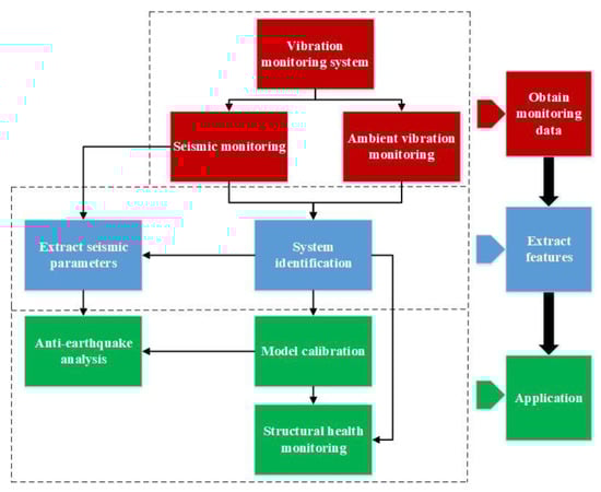
Figure 1. Application of the vibration monitoring data of concrete dams.

In this study, the modal identification of structures is compared and studied based on the seismic monitoring of dams, considering the Pacoima Dam as an example. Fundamental theories of different modal identification methods are introduced before analyzing the differences between different system identification results of methods and the induced causes. This was achieved by first sorting out the modal identification results of the Pacoima Dam from previous studies through different identification methods and comparing the system identification results based on FVTs and the finite element method (FEM). The linear time-invariant (LTI) modal identification, i.e., the input–output (IO) and output-only (OO) methods, as well as the linear time-varying (LTV) modal identification method, were separately adopted to identify the modal parameter identification of the Pacoima Dam and to compare and study the differences. The findings of this study would provide a reference for the selection of modal parameter identification methods of concrete dam modal identification and the analysis of system identification results based on strong earthquake observation in practical engineering.

2. Review of the Modal Identification Methods

In structural modal identification, it is generally assumed that the structural system is LTI, which implies that the system parameters do not change over time. The studies related to the system identification of dams using seismic monitoring are shown in Table 1.

Table 1. Statistics on the modal identification of concrete dams based on seismic observations.

Country /Region	Project Name	Height (m)	Modal Id. Method	Application of System Identification Results			FVT	AVT
				Seismic Parameter Extraction	Model Calibration	Damage Diagnosis
China	Ertan arch dam [18]	240	ARX	✔	✔			✔
	Shuikou gravity dam [19]	101	BSS	✔	✔	✔		✔
	Longyangxia arch dam [20]	178	PP	✔			✔	✔
	Xiluodu arch dam [21]	2855	SSI					✔
Taiwan, China	Fei-Tsui arch dam [22]	122.5	ARX	✔		✔	✔	✔
Switzerland	Emosson arch dam [23]	180	PP		✔	✔	✔	✔
	Mauvoisin arch dam [24]	250	PP		✔		✔	✔
	Punt-dal-Gall arch dam [24]	130	PP		✔		✔	✔
Japan	Kurobe arch dam [11]	186	FDD					✔
	Tagokura gravity dam [11]	145	FDD					✔
	Hitotsuse arch dam [25]	130	PP					✔
Portugal	Cabril arch dam [14]	132	FDD	✔	✔			✔
	Cahora Bassa arch dam [14]	170	FDD	✔	✔			✔
	Baixo Sabor arch dam [14]	123	FDD	✔			✔	✔
Iran	Karun IV arch dam [26]	230	FDD	✔	✔			✔

In FVTs of concrete dams, the commonly used system identification method includes curve fitting of frequency response functions (FRFs) or transfer functions (TFs). Table 1 demonstrates that the current seismic monitoring-based system identification of concrete dams mostly relies on the peak pick-up technique (PP) from power spectrum density (PSD), frequency domain decomposition (FDD), and the autoregressive model with exogenous terms (ARX). In addition, blind source separation (BSS) and the stochastic subspace identification (SSI) method have some application too. Alves et al. [27] proposed a modal identification method, MODE-ID, for concrete dams using an optimization algorithm. Bukenya et al. [28] made a literature review of the modal identification of dams. Classified from the way the model is built, the modal identification methods can be divided into IO-type and OO-type methods. For practical engineering issues, the input mechanism of seismic waves is very complicated and therefore requires some simplifications to be made. As shown in Figure 2, IO-type identification methods consider the seismic record of the free field of the dam foundation as the model input and the seismic response record on the dam body as the model output. In essence, in this case the foundation is regarded as rigid, and the seismic motion is applied to the dam body in the form of supporting excitation. The system identification results are the modal parameters of the dam body. When the IO-type methods are used for analysis, the uniform input form can be adopted, which means that the foundation of the dam is regarded as rigid, and the earthquake monitored by the free field of the dam foundation acts on the dam body in the form of a uniform input. The system identification results are the modal parameters of the dam body. If several strong-motion seismographs are set on the dam foundation, non-uniform input can be adopted, and the earthquake measured in different parts of the dam foundation is the input of the system. OO-type identification methods take the seismic monitoring data of the free field of the dam foundation and the dam body as the input. The seismic excitation is assumed to be random white noise, and the identified results are modal parameters of the reservoir–dam–foundation system. Because seismic excitation is generally not stationary white noise, the system identification results of this method need to exclude the dominant frequency contained in the seismic excitation.

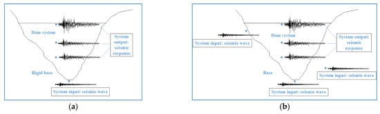
Figure 2. The input–output system of a concrete dam: (a) uniform support excitation; (b) non-uniform multiple-support excitation.

2.1. ARX

The ARX model with multiple inputs and a single output (MISO) is defined as follows:

$$A(q)y(t)=B_1(q)u_1(t-n{k}_1)+\dots +B_{nu}{u}_{nu}(t-n{k}_{nu})+e(t)$$

(1)

where $y(t)$ represents the single output; $u_i(t)$ represents the i-th input; nk_i represents the delay in the system from input $u_i(t)$ to the output; nu is the number of inputs; $A(q)$ and $B_i(q)$ are polynomials of the orders $n_a$ and $n_{bi}$, $A(q)=1+{\displaystyle \sum _{s=1}^{n_a}{a}_s{q}^{-s}}$, $B_i(q)={\displaystyle \sum _{s=1}^{n_{bi}}{b}_{si}{q}^{-s}}$, i = 1, 2, …, nu; and $e(t)$ represents the noise interference.

By minimizing the error between the structural seismic response predicted by the above model and the measured seismic response, the coefficients of the model could be derived. After finding out the roots, qm, m = 1, 2, …, n, of the polynomial A(q), the structural frequency, $f_m$, and damping ratio, ${\xi }_m$, can be obtained using the following equations:

$$f_m=\frac{\left|\ln \left(q_m\right)\right|}{2\pi \mathsf{\Delta }t}, {\xi }_m=-\frac{\mathrm{Re}\left(\ln \left(q_m\right)\right)}{\left|\ln \left(q_m\right)\right|}$$

(2)

where $\mathrm{Re}\left(\ln \left(q_m\right)\right)$ is the real part of $\ln \left(q_m\right)$ and $\mathsf{\Delta }t$ is the time interval of sampling.

It is easy to extend the above model to the multiple input/multiple output (MIMO) ARX model [18]. If the system input is white noise, the ARX model is simplified into the AR model.

2.2. FDD

FDD, which is the most widely applied method, is a frequency domain class modal identification method. It is an evolved version of the PP technique. Extended frequency domain decomposition (EFDD) is an improved version of FDD [29]. As the FDD technique is based on using a single frequency line from fast Fourier transform analysis (FFT), the accuracy of the estimated natural frequency depends on the FFT resolution, and no modal damping is calculated. However, the EFDD technique gives an improved estimation of both the natural frequencies and the mode shapes and includes the damping ratios. In addition to EFDD, the frequency domain decomposition renovated by the wavelet transform (FDD-WT) is also another method to improve FDD.

If the input of an LTI system is white noise, the power spectral density function, $G_{yy}(j\omega )$, of the output response signal, y(t), of l channels can be expressed as:

$$G_{yy}(j\omega )=H^{*}(j\omega )G_{xx}{H}^T(j\omega )$$

(3)

where $G_{xx}$ is the input signal power spectrum matrix; $H(j\omega )$ is the frequency response function matrix; ${(•)}^{\ast }$ represents the matrix of a complex conjugate; ${(•)}^{\mathrm{T}}$ represents the matrix of the transpose; and j represents an imaginary unit.

At the m-order mode, Equation (3) can be simplified to:

$$\underset{\omega \to {\omega }_m}{G_{yy}^T(j\omega )}\approx {\phi }_m\left[diag\left(2\mathrm{R}\mathrm{e}\left(\frac{c_m}{j\omega -{\lambda }_m}\right)\right)\right]{\phi }_m^T$$

(4)

where ${\phi }_m$ is the m-th-order vibration mode shape vector; $diag(\cdot )$ is the diagonal matrix; $c_m$ is a real scalar; and ${\lambda }_m$ is the m-th-order pole.

According to the response signals measured in each channel, it is estimated that the spectra and the spectral density of each signal need to be calculated before the singular value decomposition (SVD) is performed.

$$[{\stackrel{⌢}{\mathbf{G}}}_{yy}({\omega }_r)]=U_r{\Sigma }_r{U}_r^{\mathrm{H}}$$

(5)

The singular spectral curve is obtained by the singular value decomposition of the power spectral density matrix of the structural response. At a specific peak value, if only the m-order mode plays a controlling role, the estimated value of the m-order vibration mode of the structure can be obtained by the unitary vector, $U_r$, which corresponds to the maximum singular value. The frequency and the damping are available in a logarithmic decay of the corresponding single degree of the freedom-dependent function (the inverse Fourier transform of the power spectrum function).

2.3. ERA and SSI

The eigensystem realization algorithm (ERA) and SSI are based on the stochastic subspace model. The equilibrium equation of the n-degree of the freedom structure vibration can be expressed in the form of a deterministic-stochastic discrete state-space model [30]:

$$\{\begin{array}{c}{z}_{k+1}=A{z}_k+B{u}_k+w_k\\ y_k=C{z}_k+D{u}_k+v_k\end{array}$$

(6)

where z_k and y_k are the system state vector and observation vector, respectively; u_k is the system excitation; w_k and v_k are the stochastic and observation noise, respectively; and A, B, C, and D are the discrete system matrix, input matrix, observation matrix, and direct transfer matrix, respectively.

When the system excitation can be substituted by Gaussian white noise, the stochastic subsystem is written as:

$$\{\begin{array}{c}{z}_{k+1}=A{z}_k+w_k\\ y_k=C{z}_k+v_k\end{array}$$

(7)

A typical ERA identification method needs an impulse response function to construct the Hankel matrix or the Toeplitz matrix, but the impulse response is difficult to obtain directly. However, a natural excitation technique (NExT) can be adopted to obtain the impulse response, such as ERA with the natural excitation technique (ERA-NExT) or ERA with the modified natural excitation technique using average Markov parameters (ERA-NExT-AVG) [31], according to the correlation function matrix, $R_i^{}=E[y_k{y}_{k+i}^T]$, between the measured responses.

The Hankel matrix is defined as:

$$H=\left[\begin{array}{cccc}{R}_0& R_1& \dots & R_i\\ R_1& R_2& \dots & R_{i+1}\\ ⋮& ⋮& \ddots & ⋮\\ R_i& R_{i+1}& \dots & R_{2i}\end{array}\right]$$

(8)

in which i is the number of data blocks in the columns.

ERA-observer/Kalman filter identification for OO systems (ERA-OKID-OO) and ERA-observer/Kalman filter identification for IO systems (ERA-OKID-IO) are improved versions of ERA based on the observer/Kalman filter identification (OKID) approach to overcome the difficulties in retrieving the system Markov parameters that can arise related to the problem of dimensionality and numerical conditioning [32]. System realization using information matrix (SRIM) is another modified version of ERA using the information matrix that is introduced, which consists of the autocorrelation and cross-correlation matrices of the shifted input and output data [33].

SSI is another class of the commonly used modal identification methods. SSI can be divided into the realization-based method and the direct method (data-driven method), which has two categories [34,35]. The realization-based method (such as SSI-COV) is similar to ERA. Data-driven SSI (SSI-Data) uses monitoring data directly, with no need for Markov parameters, to obtain the reasonable estimations of matrices A, B, C, and D (IO-type method) or A and C (OO-type method). Due to the use of robust numerical tools such as QR decomposition and singular value decomposition (SVD), these identification techniques are often implemented for multivariable systems. The implementation algorithm of the SSI-Data method mainly includes multivariable output-error state-space (MOESP), the numerical algorithms for subspace state-space system identification (N4SID) methods, and canonical variation analysis (CVA). This study only introduces the N4SID implementation algorithm. In order to remove spurious modes, stabilization graphs were plotted [36].

2.4. Time-Varying Modal Identification Using RSSI

If considering the time-variant features of a dam structural system during an earthquake, the time-variant modal identification method could be adopted, and the system identification results of the corresponding modal parameters can be obtained at each sampling moment. The recursive ARX model (RARX) and its improved version, adaptive forgetting through multiple models (AFMM), were proposed by Gong [37]. The most commonly used LTV modal identification method is recursive SSI (RSSI).

For the LTV system, the estimation expression of the Hankel matrix shown in Equation (8) is no longer valid. Thus, the Hankel matrix $H(t)$ at time instant t should be updated online to identify the time-varying modal parameters from the vibration measurement. If the Hankel matrix $H(t-1)$ is available for the newly incoming data vector $y_t$, the new Hankel matrix $H(t)$ can be updated using the sliding window method or the forgetting factor method. For each time step, if the SVD is performed, the computation consumes too much processing power. Based on the extended instrumental variable version of the past (EIV-Past) algorithm [38,39], in order to avoid the time-consuming SVD, an unstrained optimization problem is solved instead:

$$\begin{array}{ll}\hfill \overline{V}\left[U_1(t)\right]& ={\Vert {\displaystyle \sum _{k=2i+1}^t{y}_k^{+}{y}_k^{-}{}^T-U_1(t)U_1^T(t){\displaystyle \sum _{k=2i+1}^t{y}_k^{+}{y}_k^{-}{}^T}}\Vert }_{\mathrm{F}}^2\\ & ={\Vert H_1(t)-U_1(t)U_1^T(t)H_1(t)\Vert }_{\mathrm{F}}^2\hfill \\ & ={\Vert H_1(t)-U_1(t){\overline{H}}_1(t)\Vert }_{\mathrm{F}}^2\hfill \end{array}$$

(9)

in which ${\Vert \cdot \Vert }_{\mathrm{F}}^{}$ represents the Frobenius norm. The orthonormal matrix $U_1(t)$ comprises the first 2n eigenvectors of the Hankel matrix at the time instant t. The two vectors are $y_k^{+}={\left[\begin{array}{cccc}{y}_{{}_{k-i+1}}^T& y_{{}_{k-i+2}}^T& \dots & y_{{}_k}^T\end{array}\right]}^T$, $y_k^{-}={\left[\begin{array}{cccc}{y}_{{}_{k-i}}^T& y_{{}_{k-i-1}}^T& \dots & y_{{}_{k-2i+1}}^T\end{array}\right]}^T$.

From the above recursive procedures, the orthonormal matrix $U_1(t)$ can be updated. Then, at the k-th time interval, the discrete state space matrix, A, and the observation matrix, C, are realized, and the modal parameters can be obtained at the time interval.

3. Pacoima Arch Dam and Its Earthquake Observation

To make a case study on the modal identification issues on concrete dams, this work considers the example of the Pacoima arch dam, which is located in San Gabriel Mountain in Los Angeles, southern California, USA. The Pacoima arch dam and the arrangement of acceleration sensors are shown in Figure 3. The height of the dam is 113 m, the top of the dam is 180 m long and 3.2 m thick, and the bottom is 30.2 m thick. Therefore the dam is classified as a medium-thick concrete arch dam [40].

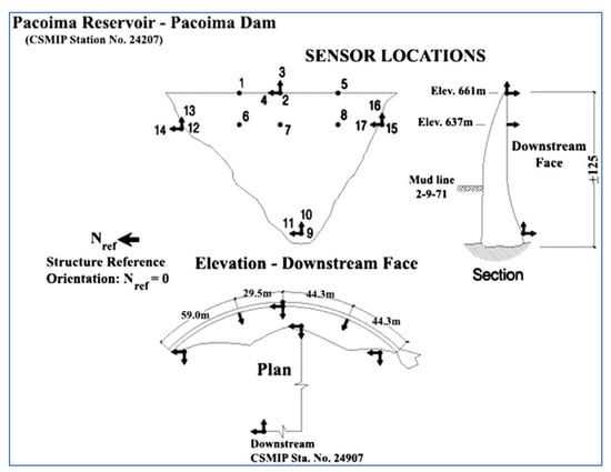
Figure 3. Pacoima arch dam and the layout of the acceleration sensors (http://www.strongmotioncenter.org/NCESMD/photos/CGS/lllayouts/ll24207.gif ) (accessed on 1 July 2021).

This area has experienced several earthquakes of different magnitudes, as shown in Table 2. Amongst them, the San Fernando earthquake on 9 February 1971 and the Northridge earthquake on 17 January 1994 were the strongest. During the San Fernando earthquake in 1971, the horizontal acceleration recorded by the accelerometer, which was installed on the left abutment 15 m above the dam top, was 1.25 g, and the peak value of the vertical acceleration was 0.7 g. A 6.35–9.7 mm crack with a depth of 13.7 m appeared between the dam and the left bank of the gravity pier. Due to the severe damage that was afflicted during the San Fernando earthquake in 1971, the dam was repaired by installing 35 steel tension cables to stabilize the upper-left abutment rock in 1976. In 1977, the dam body, foundation, and abutment of the Pacoima arch dam were assigned 9 acceleration sensors and 17 observation channels, as shown in Figure 3. Observation channels 1–8 were located on the dam body, 9–11 were located on the base rock, and 12–17 were on the right and left shoulders, which were at 80% of the dam height (elevation 637 m). The measurement direction of channels 1, 2, 5, 6, 7, 8, 9, 12, and 15 was in the radial direction, and channels 4, 11, 14, and 17 were in the tangential direction, while channels 3, 10, 13, and 16 were in the vertical direction. The structural damage caused by the Northridge earthquake on 17 January 1994 was more severe than that in the San Fernando earthquake in 1971. This earthquake caused a 50 cm downstream sliding of the thrust pier, and the horizontal opening of the expansion seam near the top of the dam was up to 5 cm. Serious cracks occurred on the left abutment of the dam [41], but no noticeable damage was found on the right abutment. After that, the dam was repaired specifically to strengthen the rocks on the left abutment. Most of the 17 channels for observing a strong earthquake at the dam could not record data due to the large seismic amplitude and high frequency. Only channels 1~3 and channels 8~11 recorded data, and the observed strong-motion sampling frequency was f_s = 50 Hz.

Table 2. The earthquakes of Pacoima arch dam.

Earthquake Name	Date	Water Level below Crest (m)	Earthquake Magnitude (Richter Scale)	Epicentral Distance from the Dam (km)	Depth of Hypocenter (km)	Horizontal Peak Acceleration (g)
						Ground	Structure
San Fernando	9 February 1971	45	6.6	8.0	9.0	1.250	-
Northridge	17 January 1994	40	6.7	18.0	19.0	1.530	2.010
San Fernando	13 January 2001	41	4.3	6.1	9.0	0.021	0.164
Chino Hills	29 July 2008	40	5.5	71.9	13.7	0.006	0.0043
Newhall	1 September 2011	-	4.2	7.8	-	0.003	0.045

After the Northridge earthquake in 1994, the strong-motion observation system was updated, and the strong-motion responses of three different earthquakes, i.e., the 2001 San Fernando earthquake, the 2008 Chino Hills earthquake, and the 2011 Newhall earthquake, were recorded. The sampling frequency of the seismic observation data was changed to fs = 200 Hz. The measurements during the San Fernando earthquake of observation channels 1, 2, 5, 6, 7, 8, 9, 12, and 15 are shown in Figure 4.

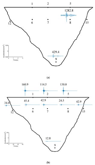
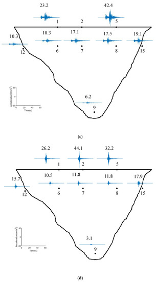
Figure 4. Earthquake responses of observation channels 1, 2, 5, 6, 7, 8, 9, 12, and 15 in the radial direction: (a) 1994 Northridge; (b) 2001 San Fernando; (c) 2008 Chino Hills; (d) 2011 Newhall.

4. Modal Identification Results Using LTI Methods

Taking the Pacoima Dam as an engineering example and combining the system identification results of the modal parameters of the Pacoima Dam obtained from various studies, the effects of various factors on the modal identification results are discussed, including the excitation, identification methods, reservoir level, and earthquake intensity as well as other factors. The reasons for the differences in the system identification results by various methods are analyzed.

4.1. Identification Results for Frequency and Damping Ratio Based on a Literature Review

The natural frequency and damping ratio of the Pacoima Dam, identified by some researchers, are shown in Table 3. Figure 5 shows the change in the second-order natural frequency of the dam over time. The following points can be derived from Table 3 and Figure 5.

Table 3. Statistics on the results of the self-resonance frequency and the damping ratio of the Pacoima arch dam by different scholars.

Num.	System Ident. by	Date	Water Level below Crest (m)	Excitation Input	Id. Method	Frequency (Hz)				Damping (%)
						1		2	3	1	2
1	Reimer [27]	July 1971	empty	Vibrator	curve fitting of FRF	5.10		5.56	-	-	-
2	ANCO Engineers [27]	April 1980	23	Vibrator	curve fitting of FRF	5.45		5.60	-	7.3	9.8
3	Alves [27]	July/August, 2002	36	Vibrator	curve fitting of FRF	5.35~5.45		5.65~5.75	-	4.0~7.0	4.5~5.5
4	Alves [27]	17 January 1994	40	Northridge earthquake	MODE-ID	undamaged	4.80	5.20	-	10.0	8.0
						damaged	3.80	4.70	-	6.0~9.0	-
5	Jalali [27]	17 January 1994	40	Northridge earthquake	ARX	undamaged	4.90	-	-	-	-
						damaged	3.90	-	-	-	-
6	Alves [42]	13 January 2001	41	San Fernando earthquake	MODE-ID	4.73~4.83		5.06	-	6.2	6.6~7.3
7	Tarinejad [43]	13 January 2001	41	San Fernando earthquake	FDD-WT	3.67		4.85	5.20	-	-
8	Tarinejad [43]	13 January 2001	41	San Fernando earthquake	4-spectral	3.60~3.70		4.80–5.00	5.10~5.30	-	-
9	Fatehi [44]	13 January 2001	41	San Fernando earthquake	ARX	4.68		5.07	-	-	-
10	Wang [45]	13 January 2001	41	San Fernando earthquake	Half-power bandwidth	-		-	-	7.0	6.7
11	Someh [44]	29 July 2008	40	Chino Hills earthquake	ARX	5.40		5.75	-	-	-
12	Alves [46]	13 January 2001	38	-	SCADA (calibrated using 2001 San Fernando earthquake)	4.82		5.02	-	-	-
13	Tarinejad [47]	29 July 2008	40	-	EACD-3D2008 (calibrated using 2008 Chino Hills earthquake)	5.43		5.60	-	-	-

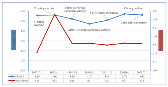
Figure 5. Evolution of the natural frequency and water levels (mode 2).

(1) The fundamental frequencies (the first-order natural frequency) of the dam identified by different scholars were different. With the excitation from a vibration generator, the fundamental frequency based on the FVT identification fell between 5.1 and 5.45 Hz. Therein, the FVT identification in 1971 was conducted in the case of an empty reservoir, and the frequency of the dam should theoretically be greater than that of a reservoir storing water. However, the FVT identification results in 1980 and 2002 were greater than that in 1971, which may be attributed to the increase in the stiffness of the dam concrete due to the contraction along the construction joints under increasing hydrostatic pressure.

(2) Okamoto [48] summarized the modal identification results of some concrete arch dams through prototype vibration tests and proposed an empirical relationship formula between the basic natural vibration period, T, of the dam and the dam height, H, as follows:

$$T=0.1+0.2\left(\frac{H}{100}\right)$$

(10)

Based on this formula, the fundamental frequency, $f=\frac{1}{T}$, of the Pacoima Dam is 3.067 Hz.

Based on the modal identification results of 40 arch dams, through a regression analysis, Kou et al. [49,50] obtained an empirical formula as follows:

$$T=\{\begin{array}{c}0.06683+0.00227H,\mathrm{for} \mathrm{mode} 1\\ \begin{array}{l}0.06658+0.00184H,\mathrm{for} \mathrm{mode} 2\\ 0.04592+0.00147H,\mathrm{for} \mathrm{mode} 3\end{array}\end{array}$$

(11)

Using this regression equation, the first three orders of natural frequency of the Pacoima arch dam were calculated to be 3.093 Hz, 3.643 Hz, and 4.716 Hz, respectively.

By comparing the empirical results expressed above with the modal identification results shown in Table 3, it can be seen that the fundamental frequencies of the Pacoima Dam identified by different scholars were obviously greater than other arch dams. It is possible that the actual first-order frequency of the structure has not been identified.

(3) When the same earthquake records were adopted for modal identification, the results from different scholars were also quite different. For example, in the San Fernando earthquake recorded in 2001, the identification results by Tarinejad were significantly smaller than those of other scholars. It should be noted that Tarinejad used an OO-type modal identification method, and the system identification results could contain a fundamental lower-order frequency. The identified fundamental frequencies based on the Northridge seismic records in 1994 were 4.8~4.9 Hz and 3.8~3.9 Hz before and after structural damage, respectively. The natural frequency of the dam abruptly changed after the Northridge earthquake in 1994, mainly because of the structural damage. The FVT results in 1980 and 2002 were consistent, and the two changes in the water level of the FVT reservoir were noted, showing that the restoration project after the 1994 Northridge earthquake recovered the overall rigidity of the dam.

(4) The system identification results of the damping ratio changed greatly, of which the first order fell between 4 and 10% and the second order fell between 4.5 and 9.8%. The identified damping of the Northridge earthquake in 1994, based on strong vibration, was bigger than several other seismic system identification results, thereby showing that the energy dissipation of the arch dam is more significant when the earthquake is strong. At present, this factor is not considered in the seismic FEM numerical analysis of arch dams. The damping ratio of the common concrete material measured by testing is generally lower than 2%, which also has considerable differences from the identification results. When the seismic intensity is low, the damping ratio is consistent or slightly bigger than when the FVT is performed. When the seismic intensity is high (e.g., in the Northridge earthquake in 1994), the natural frequency of the arch dam reduces significantly, while the damping ratio increases by up to 6~10%. Similar analysis results for the damping were obtained at some other arch dams. For example, the identified damping ratio of the Fei-Tsui arch dam, Emosson arch dam, and Mauvoisin arch dam are below 4% when using FVT, but the damping increases to 8–15% under the excitation of strong earthquakes. The main reason for the difference might be the discrepancy in the vibration magnitudes and the peak acceleration under the different excitations. Therefore, the opening degree of the horizontal seam of the arch dam, the dislocation of the foundation rock fault, and the non-linearity of the earthquake are different.

(5) Based on the modal identification results of the San Fernando earthquake in 2001, Alves modified the linear FEM model. The FEM model was built using the Smeared Crack Arch Dam Analysis (SCADA) software. Based on the identified modal parameters that were recorded in the Chino Hills earthquake in 2008, Tarinejad modified the linear FEM model that was built using the EACD-3D2008 software. The errors between the structural frequency and the modal identification results calculated by the modified model are relatively small. The calculated results of the FEM model and the modal identification results are different, which is mainly caused by the error in the FEM simulation. The FEM model is limited by many uncertain factors, such as the interception of the complex boundary conditions and the selection of the structural physical parameters, which might incorporate some errors. It is necessary to modify the model according to the modal identification results based on seismic monitoring.

4.2. Identification Results Comparison for the Frequency and Damping Ratio Using Different Methods

4.2.1. Identification Results Using OO-Type Method

The identified first four ordered frequency and the damping ratio using all seismic monitoring channel data of the dam body and the dam foundation and some OO-type methods are shown in Table 4. The identified frequency and damping using only the seismic monitoring channel data of the dam body are presented in Table 5. It is essential to determine how to eliminate the dominant frequency of seismic waves. In this work, stabilization diagrams are used. Figure 6 describes the stabilization diagram corresponding to the ERA-OKID-OO and N4SID-OO method. Since the dynamic property of the dam obviously varies over time, the earthquake record of the 1994 Northridge earthquake was not analyzed using the LTI modal identification methods.

Table 4. Modal identification results of the identified frequency and damping using all seismic monitoring channel data of the dam body, dam foundation, and OO-type method.

Earthquake	ID. Method	Frequency (Hz)				Damping (%)
		1	2	3	4	1	2	3	4
2001 San Fernando	AR	3.52	4.45	5.25	6.14	2.88	0.98	2.78	5.69
	ERA-NExT	3.55	4.35	5.17	6.23	1.71	2.44	1.81	1.03
	ERA-NExT-AVG	-	4.37	5.23	6.24	-	7.74	2.30	2.48
	ERA-OKID-OO	3.52	4.38	5.16	6.15	9.44	2.46	1.98	5.41
	N4SID-OO	3.47	4.43	5.17	6.23	6.75	1.38	1.57	1.28
	EFDD	3.42	4.39	5.19	6.15	4.55	5.03	4.39	4.78
2008 Chino Hills	AR	3.91	4.34	5.31	-	9.38	8.37	5.88	-
	ERA-NExT	3.73	4.26	5.29	-	5.91	5.33	4.96	-
	ERA-NExT-AVG	3.88	4.26	5.41	-	4.40	3.45	1.13	-
	ERA-OKID-OO	3.85	4.23	5.31	-	9.66	5.46	5.88	-
	N4SID-OO	3.73	4.20	5.22	-	6.06	8.80	6.83	-
	EFDD	3.71	4.29	5.37	6.05	4.15	3.66	5.76	1.55
2011 Newhall	AR	-	4.20	5.65	6.79	-	1.52	1.96	3.16
	ERA-NExT	-	4.26	5.66	6.87	-	2.89	1.18	0.67
	ERA-NExT-AVG	-	4.27	5.70	6.82	-	4.75	1.38	1.66
	ERA-OKID-OO	-	4.27	5.59	6.79	-	7.58	3.22	3.90
	N4SID-OO	-	4.28	5.70	6.92	-	6.03	4.13	5.98
	EFDD	-	4.20	5.66	6.83	-	0.16	3.11	3.72

Table 5. Modal identification results of the identified frequency and damping using only seismic monitoring channel data of the dam body and the OO-type method.

Earthquake	ID. Method	Frequency (Hz)				Damping (%)
		1	2	3	4	1	2	3	4
2001 San Fernando	AR	3.58	4.34	5.13	6.25	9.20	8.00	2.59	3.83
	ERA-NExT	3.59	-	5.21	6.27	2.73	-	1.59	2.54
	ERA-NExT-AVG	3.66	4.30	5.32	6.14	4.88	6.71	3.98	2.93
	ERA-OKID-OO	3.58	4.33	5.15	6.30	9.20	7.52	2.87	2.88
	N4SID-OO	3.56	4.41	5.24	6.18	9.50	8.85	3.47	2.42
	EFDD	3.42	4.39	5.19	6.15	4.29	4.15	4.61	4.91
2008 Chino Hills	AR	3.88	4.16	5.30	-	3.88	7.19	6.40	-
	ERA-NExT	3.78	-	5.33	-	5.69	-	9.79	-
	ERA-NExT-AVG	3.79	4.23	5.26	-	8.66	7.13	4.80	-
	ERA-OKID-OO	3.83	4.17	5.30	-	8.93	7.33	6.41	-
	N4SID-OO	3.97	4.36	5.37	-	6.65	6.87	5.95	-
	EFDD	3.71	4.29	5.37	6.05	1.28	3.41	3.88	2.00
2011 Newhall	AR	-	4.27	5.64	6.79	-	4.02	3.14	2.82
	ERA-NExT	-	4.24	5.65	6.83	-	2.34	2.05	0.77
	ERA-NExT-AVG	-	4.22	5.71	6.84	-	4.38	1.70	3.31
	ERA-OKID-OO	-	4.27	5.72	6.84	-	2.71	9.66	2.99
	N4SID-OO	-	4.23	5.71	6.85	-	4.98	2.66	1.96
	EFDD	-	4.20	5.66	6.83	-	4.42	3.22	3.22

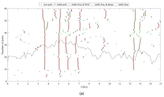
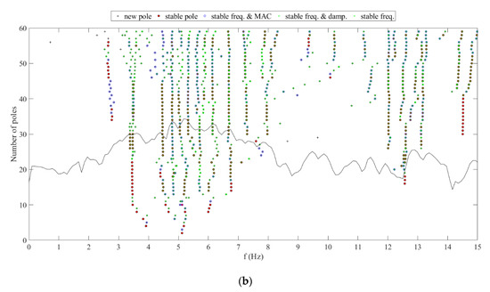
Figure 6. Stabilization diagram corresponding to different methods of modal identification in the San Fernando earthquake in 2001: (a) ERA-OKID-OO method; (b) N4SID-OO method.

(1) Compared with Table 4 and Table 5, one can see that no more order modes can be identified by using all the observation channel data. This indicates that, while only the observation channel of the dam body was used for modal identification, the system identification results would include the effect of the foundation. Therefore, the modal parameters obtained by the OO-type identification methods can be regarded as the modal parameters of the “dam-reservoir-foundation” system. Since, in theory, using more observation channels can improve the accuracy of modal identification, in the following section, only the identification results using all seismic monitoring channel data are discussed.

(2) Using different seismic records, the modal identification results showed significant differences. The identified fundamental frequency based on the Newhall earthquake in 2011 was greater than those of the other earthquakes. There are apparent differences between the system identification results identified by some methods and other methods, which may be caused by the calculation errors of the corresponding methods. Some OO-type modal identification methods depend significantly on the assumption that the excitation is steady. However, seismic waves are unsteady, and the violation of this assumption reduces the accuracy of the modal identification results.

(3) Similar to the modal identification results by Tarinejad in Table 3, the structural first-order natural frequency obtained by the OO-type identification method was smaller. For the San Fernando earthquake in 2001, the fundamental frequency was mostly below 3.8 Hz. The identified fundamental frequency based on the Newhall earthquake in 2011 was higher than that of the other earthquakes. Overall, considering the changes in the water level and seismic intensity, the greater the seismic excitation intensity, the higher the water level and the smaller the fundamental frequency.

(4) The system identification results of the damping ratio varied greatly, which was mainly caused by the high complexity of the damping characteristics of the dam structure.

4.2.2. Identification Results for IO-Type Method

Considering the spatial variability of the input excitation, both the multi-input and single-input system models were employed in input/output modal identification. Figure 7 shows diagrams of the frequency response functions calculated from four different seismic records. For the IO-type modal identification methods, when the foundation free field data input exhibits a weak coherence with the output data of the dam body, an improved IO-type model will not be built. Consequently, the IO-type recognition accuracy of the modal identification method will be significantly affected, and the identification results will yield some interference.

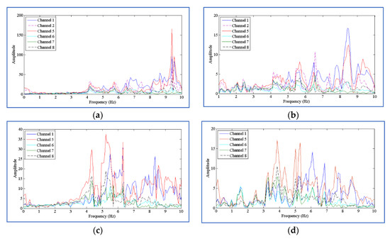
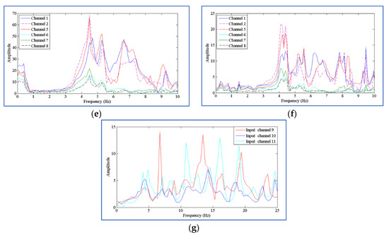
Figure 7. Structural frequency response function with different inputs: (a) 2011 Newhall earthquake, input: channel 9, output: channels 1, 5, 6, 7, and 8; (b) 2011 Newhall earthquake, input: channel 15, output: channels 1, 5, 6, 7, and 8; (c) 2008 Chino Hills earthquake, input: channel 9, output: channels 1, 5, 6, 7, and 8; (d) 2008 Chino Hills earthquake, input: channel 15, output: channels 1, 5, 6, 7, and 8; (e) 2001 San Fernando earthquake, input: channel 9, output: channels 1, 5, 6, 7, and 8; (f) 2001 San Fernando earthquake, input: channel 15, output: channels 1, 5, 6, 7, and 8; (g) 1994 Northridge earthquake, input: channels 9, 10, and 1; output: channel 8.

Table 6 and Table 7 are the system identification results of the frequency and damping with uniform input and non-uniform input, respectively. Figure 8 describes the comparison of the system identification results of the natural frequency by different identification methods using four different seismic records. From the figures and tables, it can be seen that:

Table 6. Record of observation channels 9, 12, and 15 of the dam foundation following the river as a uniform input; record of observation channels 1, 2, 5, 6, 7, and 8 of the dam body following the river as the output; and the system identification results of frequency and damping.

Earthquake	ID. Method	Frequency (Hz)				Damping (%)
		1	2	3	4	1	2	3	4
2001 San Fernando	ARX	-	4.32	5.15	6.17	-	4.59	4.06	5.49
	ERA-OKID-IO	-	-	-	-	-		-	-
	SRIM	3.50	4.27	5.28	6.19	3.39	8.87	1.33	0.71
	N4SID-IO	-	4.28	5.22	-	-	5.50	3.47	-
2008 Chino Hills	ARX	-	4.16	5.29	-	-	7.39	6.09	-
	ERA-OKID-IO	-	4.15	5.26	-	-	7.09	6.50	-
	SRIM	-	4.17	5.29	-	-	7.72	1.46	-
	N4SID-IO	-		5.32	5.91	-	-	8.19	5.30
2011 Newhall	ARX	-	4.20	-	5.80	-	6.10	-	6.89
	ERA-OKID-IO	-	-	-	-	-	-	-	-
	SRIM	3.18	4.25	-	5.61	3.25	1.77	-	7.27
	N4SID-IO	-	-	-	5.67	-	-	-	3.34

Table 7. Channels 9~17 of the dam foundation as a non-uniform input, the record of observation channels 1~8 of the dam body as the output, and the system identification results of frequency and damping.

Earthquake	ID. Method	Frequency (Hz)				Damping (%)
		1	2	3	4	1	2	3	4
2001 San Fernando	ARX	-	4.33	5.08	6.16	-	2.18	3.79	2.31
	ERA-OKID-IO	-	4.28	5.04	-	-	6.18	3.01	5.01
	SRIM	3.47	4.27	5.15	6.19	1.90	1.61	0.89	2.07
	N4SID-IO	3.59	-	5.27	-	2.98	8.78	4.17	3.77
2008 Chino Hills	ARX	3.35	-	5.14	5.87	9.75	-	8.11	1.22
	ERA-OKID-IO	-	-	5.14	5.70	-	-	4.63	4.40
	SRIM	3.23	4.19	5.14	-	0.56	1.42	1.64	-
	N4SID-IO	-	-	5.17	5.80	-	-	6.30	3.99
2011 Newhall	ARX	-	-	-	5.80	-	-	2.94	-
	ERA-OKID-IO	-	4.18	-	5.63	-	9.74	3.97	-
	SRIM	3.21	4.15	-	5.74	3.10	2.20	0.66	1.61
	N4SID-IO	-	-	-	5.73	-	-	3.96	4.71

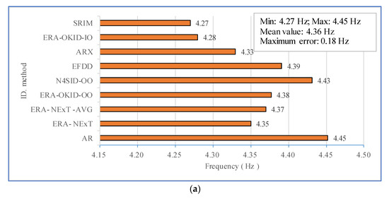
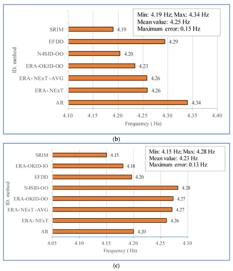
Figure 8. Mode 2 frequency obtained by the different identification methods: (a) 2001 San Fernando earthquake; (b) 2008 Chino Hills earthquake; (c) 2011 Newhall earthquake 2011.

(1) Comparing Table 6 with Table 7, in the case of non-uniform input, the identification ability of the various modal identification methods was better, and more multi-order modal parameters were identified. In the following section, only the identification results shown in Table 7 are analyzed.

(2) Comparing Table 7 with Table 4, for the same seismic monitoring, the OO-type method generally identified more order modes because the modal parameters corresponding to the dam foundation (not the modal frequency of the dam body) might be identified using OO-type methods.

(3) In three earthquakes, the fundamental frequency identified from the San Fernando earthquake in 2001 was approximately 3.2~3.6 Hz, and the damping ratio fluctuated greatly; the first-order frequency identified from the Chino Hills earthquake was approximately at 3.7 Hz, the second-order frequency was approximately 5.2~5.4 Hz, the third-order frequency was approximately 5.5~5.7 Hz, and the damping ratio fell between 4.5~6.7%; and the second-order frequency identified from the Newhall earthquake was approximately 5.6~5.8 Hz, and the damping ratio fell between 5.6~6.7%.

4.3. Identification Results Comparison for Modal Shapes

Figure 9 shows a comparison between the first-order symmetric vibration modes and the first-order anti-symmetric vibration modes of the dam body, indicating that the vibration modes identified by the different researchers exhibit some differences, but the basic shapes of the vibration modes do not differ significantly.

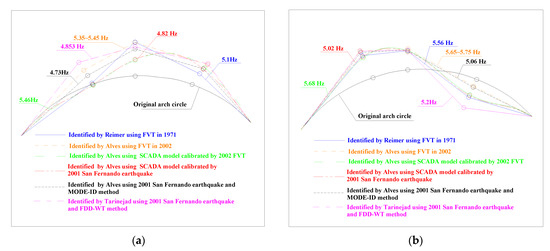
Figure 9. Comparison of the system identification results of the vibration modes in the literature: (a) the first-order symmetric vibration mode; (b) the first-order anti-symmetric vibration mode.

The first-order symmetric vibration modes of the arch dam identified by MODE-ID, SRIM, ERA-OKID-OO, and N4SID-IO using 2001 San Fernando seismic records, were compared with the mode shape calculated using FEM and that identified by FVT in 2002, as shown in Table 8. The modal confidence factor (MAC) was used to quantitatively analyze the differences between the vibration modes. From Table 8, it can be derived that, even if the FEM model was modified by the seismic system identification results, the error between the vibration modes calculated by the modified FEM model and the modal identification was still significant, which further reveals that the FEM numerical simulation of the concrete dams still yields some model errors. The accuracy of the model calibration using the identified natural frequencies is not enough.

Table 8. Comparison between the identified first-order symmetric vibration modes based on San Fernando seismic monitoring in 2001 and the analysis results of FVT and FEM.

ID. Method	FEM	2002 FVT
MODE-ID	MAC = 0.708	MAC = 0.900
SRIM	MAC = 0.876	MAC = 0.950
ERA-OKID-OO	MAC = 0.818	MAC = 0.849
N4SID-IO	MAC = 0.872	MAC = 0.912

For four modal identification methods, MODE-ID, SRIM, ERA-OKID-OO, and N4SID-IO, the comparison of the first-order symmetric vibration modes is shown in Figure 10. The errors between the vibration modes obtained by these four modal identification methods were relatively small, which reveals that the system identification results of the vibration modes of the various methods can be verified by each other.

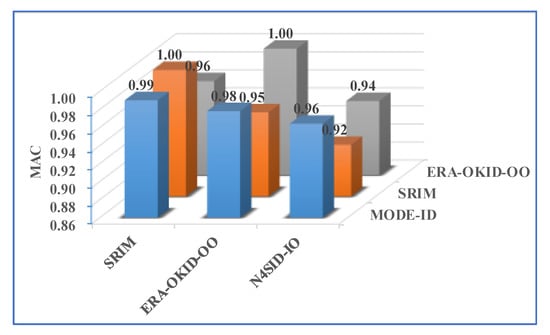
Figure 10. Comparison between the first-order symmetric vibration modes identified by San Fernando seismic monitoring in 2001 using different methods.

5. Modal Identification Using LTV Methods

Under the excitation of strong earthquakes, the interaction of a “dam-reservoir-foundation” system may cause time-variant characteristics due to the non-linearity of the dam body and dam foundation materials and the opening and closing of the horizontal seam of the dam [39]. Based on seismic records, one scheme of the time-variant modal parameter identification of concrete dams is dividing the whole seismic process into several typical periods and treating the system as an LTI system in each period. The modal identification method of LTI is adopted for the analysis of each period. This method is effective when the structural system is slowly changing. Dividing time can be realized by the method of equal time intervals (e.g., 1 s per period) or the characteristics of seismic waves (i.e., according to the arrival time of S waves). For example, Alves and Tarinejad analyzed and considered that the Pacoima Dam showed time-variant features in the Northridge earthquake in 1994 and the San Fernando earthquake in 2001. Alves [27] employed the modal identification program MODE-ID to analyze the San Fernando seismic record in 2001. Using overlapping 4 s windows ranging between 4 s and 22 s into the seismic record, the windows were overlapped so that there was a window centered every second from 6 s to 20 s into the record. For the Northridge earthquake in 1994, a window was over the first 3.2 s of the earthquake, before the arrival of the shear wave pulse. After the arrival of the shear wave, three 2 s non-overlapping windows between 4.8 s and 10.8 s were used to identify the system. Someh [44] conducted similar research using an ARX model method and a different time window length. For the Northridge earthquake in 1994, the seismic records were windowed as “before the main shock” (0–3 s), “main shock” (3–5 s), and “after the main shock” (5–8 and 8 s–end) portions to evaluate the time variation of the modal parameters. For the San Fernando earthquake in 2001, the modal identification was implemented by using “before main shock” (0–6.5 s), “main shock” (6.5–13 s), and “after main shock” (13–20, 20–27, 27–34, and 34 s–end) non-overlapping windows of the records. The time-varying natural frequency identification results of the Pacoima arch dam obtained by Alves and Tarinejad are shown in Figure 11.

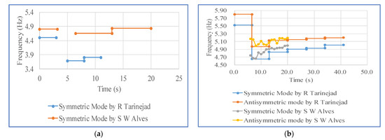
Figure 11. Time-variant frequency identification results of seismic records obtained by Tarinejad and Alves: (a) 1994 Northridge earthquake; (b) 2001 San Fernando earthquake.

Another method of time-varying modal identification is the method of recursive modal parameter identification. The RSSI method was used to identify the variation in the natural frequency of the Pacoima Dam in the San Fernando seismic records. Table 5 shows that the natural frequencies identified using the SSI method, i.e., N4SID-IO, were constant during the whole earthquake. The constant values for the first four natural frequencies were 3.56 Hz, 4.41 Hz, 5.24 Hz, and 6.18 Hz, respectively. Figure 12 shows the time-variant features of the arch dam during the earthquakes when the RSSI method was adopted. When the amplitude of the acceleration response was large, the frequency of the dam body decreased after the earthquake. The decrease in structural stiffness during the earthquake might have been caused by the decrease in the structural frequency, which needs to be further studied in the future.

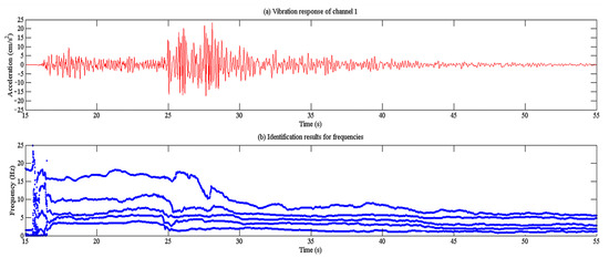
Figure 12. Variation in the structural frequency of the Pacoima Dam identified by the RSSI method during the San Fernando earthquake in 2001.

6. Conclusions

This study analyzed different modal identification results of the Pacoima arch dam using different seismic records and identification methods. After comparing these different identification results, the main conclusions can be summarized as follows:

(1) Using different excitation manners, such as FVT, AVT, and earthquake, the modal identification results had some differences. The identified modal parameters based on different seismic records also exhibited some differences. In this case, the vibration amplitude of seismic excitation was a vital factor. When the seismic excitation is strong, the jointing seam of the concrete dam may open. The dam and foundation material show apparent non-linearity, and the energy dissipation of the arch dam is more obvious when the damping of the structure is bigger. Thus, the modal identification results of the dam have some relevance to the excitation, which brings many difficulties for structural health monitoring and model calibration.

(2) The dynamic characteristics of concrete dams during big earthquakes vary over time. In particular, when the amplitude of the acceleration response is relatively large, the time-varying characteristics of the arch dam during earthquakes can be observed. The vibration amplitude of the seismic excitation should be considered during the selection of the identification methods of the modal parameters. For strong earthquakes, identification methods of time-variant modal parameters are more suitable for the analysis. One possible solution is to use the AFMM algorithm to determine whether the structural system has time-varying characteristics before modal parameter identification.

(3) The significant changes in the modal parameters of the Pacoima Dam before and after the Northridge earthquake indicate that the structural modal parameters can be used as an index for structural health diagnosis. However, the damage sensitivity of the modal parameters with minimal structural damage needs to be further investigated.

(4) Using different identification methods, the modal identification results had some differences. Thus, the modal identification results of a dam have some relevance for the choice of the identification method. How to choose an appropriate method with sufficient accuracy is an important problem that needs to be studied in the future. It suggests using a variety of different modal identification methods to verify each other and discarding the results that differ greatly from the other methods.

(5) The mode of concrete dams is very dense and the difference between two adjacent modes is very small. In addition, among all the modes, not every mode can always be identified. Thus, how to determine the actual mode order of the structure corresponding to each identified mode is a very important problem. In order to evaluate the identification results of the modal parameters, in addition to the mutual verification of the results of various modal identification methods, we suggest comparing the identification results of modal parameters with the empirical results shown in Formulas (10) and (11) as well as the results of finite element numerical simulation to judge if the modes have been correctly identified.

(6) The identified modal parameters based on the measured vibration response exhibit some differences compared to the results calculated by the FEM method. Modeling calibration is a classical step in static conditions through monitoring results comparisons. In dynamic conditions it remains more difficult and needs more research.

References

- Hansen, K.D.; Nuss, L.K. Lessons learned from the earthquake performance of concrete dams. Int. Water Power Dam Constr. 2011, 63, 32–34, 36–37. [Google Scholar] [CrossRef]
- Hall, J.F. The dynamic and earthquake behaviour of concrete dams: Review of experimental behaviour and observational evidence. Soil Dyn. Earthq. 1988, 7, 58–121. [Google Scholar] [CrossRef]
- Chopra, A.K. Earthquake analysis of arch dams: Factors to be considered. J. Struct. Eng. 2012, 138, 205–214. [Google Scholar] [CrossRef]
- Tarinejad, R.; Ahmadi, M.T.; Harichandran, R.S. Full-scale experimental modal analysis of an arch dam: The first experience in Iran. Soil Dyn. Earthq. Eng. 2014, 61–62, 188–196. [Google Scholar] [CrossRef]
- Birtharia, A.; Jain, S.K. Applications of ambient vibration testing: An overview. Int. Res. J. Eng. Technol. 2015, 02, 845–852. [Google Scholar]
- Bukenya, P. Ambient Vibration Testing of Concrete Dams. Master’s Dissertation, University of Cape Town, Cape Town, South Africa, 2011. [Google Scholar]
- Cheng, L.; Yang, J.; Zheng, D.J. The Health Monitoring Method of Concrete Dams Based on Ambient Vibration Testing and Kernel Principle Analysis. Shock Vib. 2015, 2015, 342358. [Google Scholar] [CrossRef]
- Cheng, L.; Yang, J.; Zheng, D.J.; Tong, F.; Zheng, S.Y. The dynamic finite element model calibration method of concrete dams based on strong-motion records and multivariate relevant vector machines. J. Vibroengineering 2016, 18, 3811–3828. [Google Scholar] [CrossRef]
- Darbre, G.R. Strong-motion instrumentation of dams. Earthq. Eng. Struct. Dyn. 1995, 24, 1101–1111. [Google Scholar] [CrossRef]
- Chen, H.Q. Important Strong Earthquake Data and Analysis of China’s Hydraulic Structure; Seismological Press: Beijing, China, 2000. (In Chinese) [Google Scholar]
- Fry, J.J.; Matsumoto, N. Validation of dynamic analyses of dams and their equipment. In Edited Contributions to the International Symposium on the Qualification of Dynamic Analyses of Dams and their Equipments; CRC Press: Saint-Malo, France, 2018. [Google Scholar]
- Darbre, G.R.; De Smet, C.A.M.; Kraemer, C. Natural frequencies measured from ambient vibration response of the arch dam of Mauvoisin. Earthq. Eng. Struct. Dyn. 2000, 29, 577–586. [Google Scholar] [CrossRef]
- Morrison, P.; Maley, R.; Brady, G.; Porcella, R. Earthquake Recordings on or Near Dams; USCOLD Committee on Earthquakes: Pasadena, CA, USA, 1977. [Google Scholar]
- Oliveira, S.; Alegre, A. Seismic and structural health monitoring of dams in Portugal. In Seismic Structural Health Monitoring; Springer: Cham, Switzerland, 2019; pp. 87–113. [Google Scholar] [CrossRef]
- Cheng, L.; Tong, F.; Li, Y.L.; Yang, J.; Zheng, D.J. Comparative Study of the Dynamic Back-Analysis Methods of Concrete Gravity Dams Based on Multivariate Machine Learning Models. J. Earthq. Eng. 2018, 2018, 1–22. [Google Scholar] [CrossRef]
- Cheng, L.; Tong, F. Application of Blind Source Separation Algorithms and Ambient Vibration Testing to the Health Monitoring of Concrete Dams. Math. Probl. Eng. 2016, 2016, 4280704. [Google Scholar] [CrossRef]
- Moyo, P.; Bukenya, P. Experiences with continuous monitoring of deformation and modal properties of an arch dam. In Proceedings of the 8th Structural Health Monitoring of Intelligent Infrastructure Conference, Brisbane, Australia, 5 December 2017. [Google Scholar]
- Yang, J.; Jin, F.; Wang, J.T.; Kou, L.H. System identification and modal analysis of an arch dam based on earthquake response records. Soil Dyn. Earthq. Eng. 2017, 92, 109–121. [Google Scholar] [CrossRef]
- Cheng, L.; Zheng, D.J. The identification of a dam’s modal parameters under random support excitation based on the Hankel matrix joint approximate diagonalization technique. Mech. Syst. Signal Process. 2014, 42, 42–57. [Google Scholar] [CrossRef]
- Zhang, L.F.; Xing, G.L.; Zhang, M. Analysis of strong earthquake of gravity arch dam in Longyang gorge. J. Hroelectric Eng. 1998, 1998, 14–17. [Google Scholar] [CrossRef]
- Li, S.; Wang, J.T.; Jin, A.Y. Parametric analysis of SSI algorithm in modal identification of high arch dams. Soil Dyn. Earthq. Eng. 2020, 129, 105929. [Google Scholar] [CrossRef]
- Loh, C.H.; Wu, T.S. Identification of Fei-Tsui arch dam from both ambient and seismic response data. Soil Dyn. Earthq. Eng. 1996, 15, 465–483. [Google Scholar] [CrossRef]
- Proulx, J.; Darbre, G.R.; Kamileris, N. Analytical and experimental investigation of damping in arch dams based on recorded earthquakes. In Proceedings of the 13th WCEE, Vancouver, BC, Canada, 1–6 August 2004. [Google Scholar]
- Chopra, A.K. Comparison of recorded and computed responses of arch dams. In Proceedings of the International Symposium on Dams, Kyoto, Japan, 23 July 2012. [Google Scholar]
- Okuma, N.; Etou, Y.; Kanazawa, K.; Hirata, K. Dynamic property of a large arch dam after forty-four years of completion. In Proceedings of the 14th World Conference on Earthquake Engineering, Beijing, China, 12–17 October 2008. [Google Scholar]
- Tarinejad, R.; Falsafian, K.; Aalami, M.T. Modal identification of Karun IV arch dam based on ambient vibration tests and seismic responses. J. Vibroengineering 2016, 18, 3869–3880. [Google Scholar] [CrossRef]
- Alves, S.W. Nonlinear Analysis of Pacoima Dam with Spatially Non-Uniform Ground Motion. Ph.D. Dissertation, Rep. EERL 2004-11 Earthquake Engineering Research Lab., CA. Inst. of Tech., Pasadena, CA, USA, 2005. [Google Scholar]
- Bukenya, P.; Moyo, P.; Beushausen, H.; Oosthuizen, C. Health monitoring of concrete dams: A literature review. J. Civ. Struct. Health Monit. 2014, 4, 235–244. [Google Scholar] [CrossRef]
- Ghalishooyan, M.; Shooshtari, A.; Abdelghani, M. Output-only modal identification by in-operation modal appropriation for use with enhanced frequency domain decomposition method. J. Mech. Sci. Technol. 2019, 33, 3055–3067. [Google Scholar] [CrossRef]
- Chang, M.; Pakzad, S.N.; Leonard, R. Modal identification using SMIT. In Topics on the Dynamics of Civil Structures; Springer: New York, NY, USA, 2012. [Google Scholar] [CrossRef]
- Chang, M.; Pakzad, S.N. Modified natural excitation technique for stochastic modal identification. J. Struct. Eng. 2013, 139, 1753–1762. [Google Scholar] [CrossRef]
- Lus, H.; Betti, R.; Longman, R.W. Identification of linear structural systems using earthquake induced vibration data. Earthq. Eng. Struct. Dyn. 1999, 28, 1449–1467. [Google Scholar] [CrossRef]
- Juang, J.N. System realization using information matrix. J. Guid. Control. Dyn. 2012, 20, 492–500. [Google Scholar] [CrossRef]
- Kim, J.; Lynch, J.P. Subspace system identification of support-excited structures-part I: Theory and black-box system identification. Earthq. Eng. Struct. Dyn. 2012, 41, 2235–2251. [Google Scholar] [CrossRef]
- Van Overschee, P.; De Moor, B. Subspace algorithms for the stochastic identification problem. Automatica 1993, 29, 649–660. [Google Scholar] [CrossRef]
- Ruben, L.B.; Joaquin, A.B. Interpretation of stabilization diagrams using density-based clustering algorithm. Eng. Struct. 2019, 178, 245–257. [Google Scholar] [CrossRef]
- Gong, M.S. Structural modal parameters identification and application based on earthquake response data. Ph.D. Dissertation, Institute of Engineering Mechanics of China Earthquake Administration, Harbin, China, 2005. [Google Scholar]
- Liu, Y.C.; Loh, C.H.; Ni, Y.Q. Stochastic subspace identification for output-only modal analysis: Application to super high-rise tower under abnormal loading condition. Earthq. Eng. Struct. Dyn. 2013, 42, 477–498. [Google Scholar] [CrossRef]
- Cheng, L.; Tong, F.; Yang, J.; Zheng, D.J. Online modal identification of concrete dams using the subspace tracking-based method. Shock Vib. 2019, 2019, 7513261. [Google Scholar] [CrossRef]
- Processed data for Pacoima Dam—Channels 8 through 11 from the Northridge Earthquake of 17 January 1994; Report OSMS 94-15 A; California Strong Motion Instrumentation Prg: Sacramento, CA, USA, 1994.
- Phase 1 data for Pacoima Dam—Channels 1-6, 12, 13 and 15-17 from the Northridge Earthquake of 17 January 1994; Report OSMS 95-05; California Strong Motion Instrumentation Prg: Sacramento, CA, USA, 1995.
- Alves, S.W.; Hall, J.F. System identification of a concrete arch dam and calibration of its finite element model. Earthq. Eng. Struct. Dyn. 2006, 35, 1321–1337. [Google Scholar] [CrossRef]
- Tarinejad, R.; Damadipour, M. Extended FDD-WT method based on correcting the errors due to non-synchronous sensing of sensor. Mech. Syst. Signal Process. 2016, 72–73, 547–566. [Google Scholar] [CrossRef]
- Someh, R.F. Modal identification of an arch dam during various earthquakes. In Proceedings of the 1st International Conference on Dams & Hydropower, Tehran, Iran, 1 January 2012. [Google Scholar]
- Wang, J.T.; Chopra, A.K. Linear analysis of concrete arch dams including dam-water-foundation rock interaction considering spatially varying ground motions. Earthq. Eng. Struct. Dyn. 2010, 39, 731–750. [Google Scholar] [CrossRef]
- Alves, S.W.; Hall, J.F. Generation of spatially nonuniform ground motion for nonlinear analysis of a concrete arch dam. Earthq. Eng. Struct. Dyn. 2006, 35, 1339–1357. [Google Scholar] [CrossRef]
- Tarinejad, R.; Fatehi, R.; Harichandran, R.S. Response of an arch dam to non-uniform excitation generated by a seismic wave scattering model. Soil Dyn. Earthq. Eng. 2013, 52, 40–54. [Google Scholar] [CrossRef]
- Okamoto, S. Introduction to Earthquake Engineering, 2nd ed.; University of Tokyo Press: Tokyo, Japan, 1984. [Google Scholar]
- Kou, L.H.; Jin, F.; Chi, F.D.; Wang, L. Analysis of prototype dynamic test of concrete arch dams at home and abroad. J. Hydroelectr. Eng. 2007, 26, 31–37. [Google Scholar] [CrossRef]
- Liu, N.F.; Li, N.; Li, G.F.; Song, Z.P.; Wang, S.J. Method for Evaluating the Equivalent Thermal Conductivity of a Freezing Rock Mass Containing Systematic Fractures. Rock Mech. Rock Eng. 2022. [Google Scholar] [CrossRef]
Publisher’s Note: MDPI stays neutral with regard to jurisdictional claims in published maps and institutional affiliations. |
© 2022 by the authors. Licensee MDPI, Basel, Switzerland. This article is an open access article distributed under the terms and conditions of the Creative Commons Attribution (CC BY) license (https://creativecommons.org/licenses/by/4.0/).