Abstract
Machine learning (ML) models are now widely used in digital twins of water treatment facilities. These models are commonly trained based on historical datasets, and their predictions serve various important objectives, such as anomaly detection and optimization. While predictions from the trained models are being made continuously for the digital twin, model updating using newly available real-time data is also necessary so that the twin can mimic the changes in the physical system dynamically. Thus, a synchronicity framework needs to be established in the digital twin, which has not been addressed in the literature so far. In this study, a novel framework with new coverage-based algorithms is proposed to determine the necessity and timing for model updating during real-time data transfers to improve the ML performance over time. The framework is tested in a prototype water treatment facility called the secure water treatment (SWaT) system. The results show that the framework performs well in general to synchronize the model updates and predictions, with a significant reduction in errors of up to 97%. The good performance can be attributed particularly to the coverage-based updating algorithms which control the size of training datasets to accelerate the ML model updating during synchronization.
1. Introduction
Digital twin, a digital replica of the physical asset which can safeguard the physical asset as well as optimize its operations, is becoming the most promising enabling technology for smart manufacturing in the Industry 4.0 concept [1,2]. Machine learning (ML) models are also widely used in the digital twinning process of cyber-physical systems for various purposes [3]. For example, Min et al. [4] integrated ML and industrial big data in their digital twin to optimize petrochemical production. Snijders et al. [5] used a temporal convolutional neural network for the digital twin of a cyber-physical energy system to predict its responsiveness to specific power setpoint instructions. In addition, Xu et al. [6] adapted a generative adversarial network model in their digital twin to detect anomalies.
In the digital twinning process, real-time model updating is essential so that the twin can continuously mimic the dynamic changes of the physical asset. However, this topic is not well addressed in the literature and only a few studies have investigated model updating of the digital twin so far. Wang et al. [7] proposed a model updating scheme based on parameter sensitivity analysis, which was basically a direct error correction between their digital twin and the physical system. Wei et al. [8] used a consistency retention method for their computer-numerical-control machine tool to detect the performance attenuation in the digital twin, and then subsequently update the finite element model. Farhat et al. [9] built a numerical model to simulate the data for ML predictive models in a digital twin, and then demonstrated the importance of the updated parameters for prediction accuracy. Adam et al. [10] further pointed out the importance of model updating to limit error amplification in a healthcare setting. However, for the real-time updating of ML models in the digital twin, there has not been any study reported in the literature as far as we are aware.
It is well known that the performance of ML models depends largely on their training datasets [11,12]. In our previous study on the anomaly detection framework for the digital twin of water treatment facilities [13], the ML model trained with one dataset performed poorly on another test dataset due to their different coverage, which was defined as the interval between the minimum and maximum target value in the dataset. In other words, if the target value has not appeared within the range in the training dataset, it is normally difficult to predict with good accuracy in the test dataset [14]. Thus, it is always desirable to continuously carry out real-time ML model updating to expand coverage so that the ML predictions in the digital twin is accurate for ongoing operations. However, this issue has not yet received proper attention and is the focus of the present study.
Computational speed is crucial for real-time model updating. If the speed is fast enough that the updating can be completed within the time step, the update can be performed continuously, and the synchronicity framework would not be needed in theory. Unfortunately, this is not the situation in most cases; hence, approaches for incremental learning need to be considered to speed up the model updating and include new knowledge with the real-time data, while inherent knowledge is maintained [15]. We importantly note that it is also possible that ML can suffer from catastrophic forgetting when learning new information incrementally [16,17,18]. For example, eXtreme Gradient Boosting (XGBoost) adopts the exact greedy algorithm to enumerate all possible splits for each tree node and to determine the best splits [19], and it is difficult for XGBoost to achieve the best splits with incremental learning [20]. Other tree-boosting methods opt to integrate new classifiers and discard outdated ones in classification tasks [21], but this approach is infeasible for regression tasks. Therefore, more research on incremental ML is still needed in the future.
In the present study, we propose a novel framework with real-time model updating to optimize the simultaneous objectives of providing predictions based on current ML models while generating updated ML models in the background. It is the first framework to deal with ML model forecasts and ML model updates in parallel, as far as we are aware. New coverage-based updating algorithms are developed to determine the sufficiency of training datasets and to speed up the updating circle. Histogram selection and area selection are also established to optimize the database for a better model-updating performance. This framework can be broadly applied to predictive models in real-time digital twins with out-of-range issues. It is tested and verified in a prototype water treatment facility called the secure water treatment (SWaT) system, hosted in iTrust in Singapore.
In the following, the details of the real-time data-processing framework and coverage-based updating algorithms are first described in Section 2. Subsequently, the prototype facility, datasets and models used in this study are introduced in Section 3. The implementation of the framework in the SWaT system is presented with discussions of training and operational parameters in Section 4. Finally, a conclusion is drawn in Section 5.
2. Materials and Methods
2.1. Real-Time Data-Processing Framework
Real-time data transfer is integral to the digital twin, and the ML models inside the twin make predictions and forecasts continuously based on the data input. At the same time, model updating must also be implemented in parallel to improve the dynamic prediction performance of the models based on the real-time data inputs. Previous studies typically implement these two procedures sequentially (e.g., Guajardo et al. [22]). However, an optimal digital twin requires both to be carried out in parallel, and thus a framework for their synchronicity is needed which is yet to be established.
In this study, we propose a real-time data-processing framework for simultaneous forecasting and model updating as shown in Figure 1. In this framework, the communications between the two processes are accomplished through two sharing flags (1 = true and 0 = false). Flag 1 controls the retraining/updating and is checked at each timestep in the updating script. When Flag 1 is true, the system examines the new data collected during the time step(s). If the new data are judged to be useful or capable of improving model insufficiency, retraining will be activated. Otherwise, no action is taken. The details of the criteria for the judgement of ‘useful data’ and ‘sufficient’, etc., are discussed in the following section.
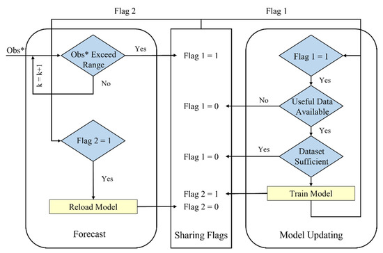
Figure 1.
Real-time model-updating framework (Obs* represents observations from digital twin and k represents timestep).
The usage of Flag 2 is more straight forward. It is set as true after each training and is written back to false after the system has reloaded the updated model. Similar to Flag 1, Flag 2 is read by the forecasting script at each timestep as shown in Figure 1. In any case, forecasting is always made by the ML models regardless of the status of Flag 2.
2.2. Coverage-Based Updating Algorithms
The judgement of whether a ML model needs retraining can be complex due to various reasons, such as sensor drifts [23,24], constant offsets [25] and low selectivity [26], as well as other reasons related to model uncertainty [27]. In this study, we focus on the reduction in model uncertainty due to the insufficient coverage of the training dataset. When operating the facility, additional new information appears from time to time with different feed inputs and reactor conditions; thus, continuous ML model updating with expanded coverages is needed for every facility.
With the digital twin, real-time information is made available continuously due to the online data transfer. As discussed above, in terms of model updating, it might not be feasible to collect all data and to train the model at every time step because such an approach is costly and prone to catastrophic forgetting, as well as computationally intensive. Previous studies used fixed time windows [22] and training subsets [28] to reduce computational complexity in the training process. In this study, we propose new coverage-based algorithms to incrementally update the training dataset by retaining the original dataset while limiting the amount of new data to be added to the datasets to shorten the computational time. The details of the algorithm are provided below.
There are two key considerations on whether the new data should be incorporated into the training dataset, i.e., whether the new data can expand the coverage of the existing dataset (called area selection) and whether the new data should be added to the insufficient bins (called histogram selection). In the algorithm, these two considerations are carried out by sequentially checking on the existing training dataset as shown in Figure 2.
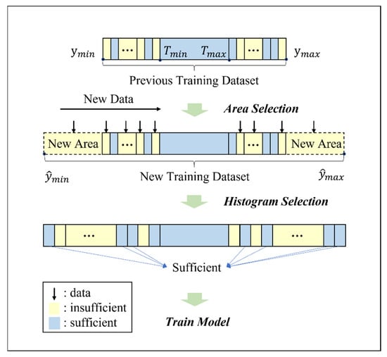
Figure 2.
Dataset evolution during the training process.
In the area selection step, if the new data appears in the out-of-range area that can expand coverage, the need for model updating will be activated as shown in Figure 2. Two new areas can be possibly added in this case: (a) the max area from the maximum target value in the original training dataset to the maximum target value in the new training dataset ; and (b) the min area from the minimum target value in the original training dataset to the minimum target value in the new training dataset .
In the histogram selection step, each new area is divided into bins with equal width, and the frequency (i.e., the number of samples) in each bin is counted as for . The bin density can then defined in terms of its frequency as:
In this framework, we choose to fix the number of bins instead of the bin width. Given that the coverage can change significantly when new data appears and thus the bin number can explode if the bin width is fixed. Subsequently, a threshold for frequency density can be set as the histogram selection criteria as follows:
No additional sample needs to be added for sufficient bins despite the availability of new data. On the other hand, new samples are incorporated in the insufficient bins when available (i.e., the new data is considered as ‘useful’ for subsequent procedures). This procedure limits the size of the training dataset in order to speed up the computational time for the model updating. In the event that the new data provides too many useful samples in the insufficient bins, a random selection is implemented as follows:
where is the number of useful samples in the insufficient bin and is the bin width. When both the area and histogram selection steps are completed, model updating will then be executed with the new training dataset.
3. Datasets and Models
3.1. Testbed and Datasets
The proposed data-processing framework was tested using datasets collected from the prototype facility of the SWaT system, which is a scaled-down water treatment testbed in iTrust [13]. More details of the setups for the SWaT system can be found in Mathur and Tippenhauer [29] and Raman et al. [30]. The SWaT system consists of six treatment stages. Each stage has multiple sensors and actuators which are controlled by operation logics in the programmable logic controller (PLC). The sensors related to chemical concentrations are critical components in water treatment facilities. However, they vary continuously and are usually difficult to predict with traditional methods, and ML models are more likely to be effective [31,32,33,34]. Here, we tested and evaluated the real-time data-processing framework based on the ML models of the sensor AIT202, which measures the pH value of the water after the chemical dosing stage. It should be noted that the framework can be implemented to all sensors in water treatment facilities, and their parameters and ML models can be specified independently. For actuators, we adopted the PLC-based whitelist system for the digital twin studied by Wei et al. [13], which used PLC logics to verify the status of actuators. These PLC logics are typically pre-established with historical data and do not need to be updated if the PLC programs are constant. Thus, this study focuses on predictive ML models built for sensors that need updates to maintain accuracy.
Three datasets were used to evaluate the framework as shown in Table 1. Dataset 1 was the original training dataset. It was collected within a short duration and thus had a narrow coverage for the target value. Dataset 2 represented the real-time operation scenario, and the data at each time step was obtained every second, according to the status of the SWaT system. The coverage-based updating algorithms were able to extract useful samples from Dataset 2 and combine them with Dataset 1 to generate new training datasets over time. Dataset 3 was a combination of multiple smaller datasets, which had more samples compared with the other two datasets, and it was used to examine the effect due to the frequency density as discussed in the following sections.

Table 1.
Size of the three datasets used in this study.
It should be noted that the real-time requirements of physical systems vary a lot. In this study, the update frequency of the SWaT system is every second, and the communication latency is within seconds, which is more advanced when compared with real-world water treatment facilities. Although computational time may not be the main concern for current facilities that collect data at a low frequency such as daily or hourly, the accelerating digitization trend will lead to changes in the near future, and the real-time concern could then become critical for them at that time.
3.2. Models and Assessment of Accuracy
The ML approach of natural gradient boosting (NGBoost) was adopted to establish the data-driven models in the digital twin described in our previous study [13]. NGBoost uses multi-parameter boosting and natural gradients to integrate the base learner, probability distribution and scoring rule into a modular algorithm for probabilistic assessment. The model can output both predictions and uncertainty estimations, and it has been found to perform well in real-time forecasting tasks for water treatment facilities, where pre-processing to reframe the time series of observations into pairs of input and output sequences is required before the training [13]. The focus of this study is on the synchronicity framework with new optimization algorithms for model updating. Details of the mathematical theories and ML model structures will not be covered here. The readers are referred to more information about the NGBoost model provided in Duan et al. [35], and its application in the anomaly detection of the digital twin in water treatment facilities in our earlier paper, conducted by Wei et al. [13].
As a tree-boosting method that partitions the data into axis-aligned slices for training, incremental training is not suitable for NGBoost as discussed in Section 1. However, NGBoost can execute with fast computational speed, which makes it efficient to retrain from scratch. In this study, only the predictions from NGBoost were evaluated in the data-processing framework for model updating, and uncertainty estimations could be used for anomaly detection in previous work [13]. It is also important to note that the framework proposed here is applicable to other ML models because the coverage-based updating algorithms can expand the useful training data over time, which can lead to an improvement in the prediction accuracy of ML models in general.
Some ML studies included feature selections and grid searches in the model updating scheme [22]. In this framework, however, these procedures are completed in the preparation stage for the digital twin because they are time-intensive for real-time tasks. For water treatment facilities with PLCs, feature selection can largely benefit from embedded logics because almost all the important relationships between sensors and actuators have been written in PLC programs. A correlation-based feature selection method [36] was also used as the supplement to evaluate the merit of features for the SWaT testbed. Then, the main network hyperparameters (see Table 2) were selected based on a grid search [37] with three-fold cross validation, and NGBoost with the five-time-step inputs was found to yield the best prediction performance according to our previous study, conducted by Wei et al. [13].
Table 2.
Hyperparameter of the NGBoost model in this study.
During real-time operations, validation datasets used in the training processes were randomly split from the whole training datasets with a rate of 20%. In addition, 2000 samples were randomly chosen in advance from Dataset 3 as the test dataset to examine the effect due to frequency density. The results in the following sections were obtained by running the subprocess module with the function Popen, and the NGBoost models were built on Scikit-learn in Python.
In this study, we evaluate the performance of the real-time data-processing framework using mean absolute error (MAE) and root mean square error (RMSE). MAE is a criterion that measures the sum of errors between the actual observation and predicted values over the entire period, and then divides the sum obtained by the number of observations as shown in Equation (4). RMSE is the standard deviation of the prediction errors and indicates the spread for the residuals as shown in Equation (5).
where is the actual observation and represents the prediction, and n is the number of time steps over this period.
4. Results and Discussion
The original performance without the implementation of the data-processing framework is used as the benchmark in all the following discussions. Dataset 1 was chosen as the original training dataset, and Dataset 2 was used to simulate the real-time operational data streams from the digital twin as mentioned in Section 3.1. Dataset 2 had a wider coverage of target values than Dataset 1, with more than four times the number of samples. Figure 3 shows the target values of both Datasets 1 and 2, with the blue area highlighting the samples within the original range [6.99, 8.24]. It can be observed that in Dataset 2, many samples were lower than the minimum of the original range and that sporadic samples were higher than the maximum. Figure 3c compares the predictions from the original ML model and the true observations from the physical system. Despite the small size of Dataset 1 for training, all the targets within the original range were well predicted by the ML model. It is also observed from Figure 3c that nearly all out-of-range samples were not predicted well due to an insufficient training dataset, with a high MAE of 0.53 for the total 3591 samples in the red area. In the following discussions, only the out-of-range area (i.e., red area in the figure) is discussed, and the training samples within the original range were not included during the real-time model updating due to their good performance.
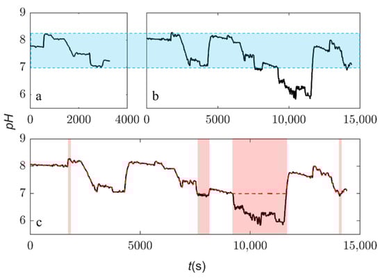
Figure 3.
Dataset information and original predictions. Title represents: (a) = Dataset 1; (b) = Dataset 2; (c) = original model performance on Dataset 2. Black solid line = observations from the physical system and red dashed line = predictions. Blue area = the range of Dataset 1 and red area = samples that are out of range.
As discussed previously, the computational time required is crucial for real-time model updating. Here, the training time of each model during the model-updating process was tracked under the conditions of frequency density = 4000 and number of bins = 10. The model was trained 139 times during the real-time simulation with operational data from Dataset 2. The training time increased progressively with expanded training datasets and was nearly double for the last training as shown in Figure 4. It should be noted that the increase in training time during the operation remained acceptable for this pilot water treatment facility, SWaT, due to the fast computational speed of the NGBoost model using a laptop processor with Intel® Core™ i7-8565U CPU @ 1.80 GHz and training datasets of a limited size. However, the general concern for time needs to be highlighted because other ML models can have a much longer training time, leading to a significant worsening of the model-updating performance. For example, deep neural networks, such as long short-term memory networks, can take ten times longer to train. Thus, optimizing the model updating, as well as utilizing faster hardware, is essential to meeting the real-time accuracy requirements.
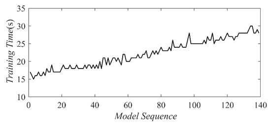
Figure 4.
Training time evolution for the model with coverage-based model-updating framework (frequency density = 4000, the number of bins = 10).
To further illustrate the impact of the computational training time, an investigation was carried out with extra time added to each training process. The predictions and observations during the period of 7000–12,000 s are shown in Figure 5a, with their differences displayed in Figure 5b, accordingly. It is obvious that the prediction error can be significant during this period. On the other hand, the prediction lines, by adopting the original training time or plus an extra 60 s, fitted the observation lines well, and the corresponding red and magenta lines in Figure 5b are always around 0. Except for these two conditions, the other prediction lines in Figure 5a are obviously jagged, particularly for the long duration between 9200 s to 11,600 s. This is because closer predictions typically occur after each reloading of the new model and before the next round of model updating, during which the existing model produces erroneous results in the out-of-range areas until the model is updated. In this framework, the model is continually retrained when new out-of-range data appears, and thus the training time decides the width of the jaggedness.
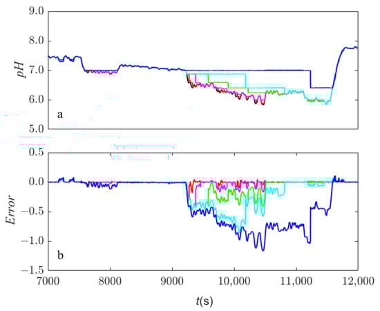
Figure 5.
Model predictions and corresponding errors using the coverage-based model-updating framework with different training speed: (a) predictions of the pH value; and (b) errors between predictions and observations. Color represents black = observations, red = original speed, magenta = extra 60 s, green = extra 300 s, cyan = extra 600 s and blue = extra 1800 s.
Table 3 summarizes the MAE between the predictions and observations with different extra training time. The MAE with real-time model updating was 0.01, indicating that 97% of out-of-range errors can be reduced because the MAE of the initial predictions was 0.53. However, the MAE increased dramatically with more extra time added to the training process, and the improvement from the model updating became negligible when the extra time reached 1800 s (see Table 3). Therefore, we can conclude that the computational training time is critical and lengthening the training time can largely increase the prediction errors.
Table 3.
Prediction accuracy with different extra time added in the model updating.
To optimize the computational training time, the size of the training dataset should be restricted in terms of its frequency density as discussed in Section 2.2; however, this restriction can also lead to a deterioration in prediction accuracy. Here, Dataset 3 was used to investigate the impact of frequency density on prediction accuracy. Samples from Dataset 3 were extracted with different intervals, and then combined as the new training datasets. During the evaluation, three models were trained with each training dataset, and their average performance is plotted in Figure 6. As expected, the performance of larger datasets (i.e., smaller extraction interval) tends to perform better with a smaller MAE and RMSE, as shown in the figure. At the same time, the variations of MAE/RMSE were small when the extraction interval was smaller than 25, as highlighted in blue area. This implies an optimal strategy to slightly sacrifice the single prediction performance for the overall improvement, with restrictions on the frequency density of the training datasets. In addition, the analysis provides a rough estimation of the suitable density for the training dataset. According to the definition of frequency density, the overall density with the extraction interval 25 was around 7000, implying that the density parameter in the algorithms can be set to be lower than 7000 because the samples in Dataset 3 were not evenly distributed.
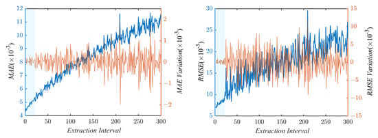
Figure 6.
MAE/RMSE and their variations on the test dataset with different extraction intervals. Blue line = MAE/RMSE and orange line = variations. Blue area indicates small variations.
Figure 7 shows the histograms of Datasets 1 and 2 with different bin widths. Unprocessed datasets are usually uneven, as shown in Figure 7. If reducing the computational training time is an exigent mission for a specific case, the samples in the original training dataset can even be screened off according to the minimum frequency density suggested above, and new samples can be added only to the sparse areas during the histogram selection step. In this case, the ML models with the original training dataset already performed well with an acceptable computational training time, and therefore the screening was not necessary. It can also be observed from Figure 7 that histograms with smaller bin width have a more accurate distribution, and their frequency can change dramatically with bin width. For example, the highest frequency of Dataset 2 with a bin width of 0.1 was ~2400, while that with a bin width of 0.02 was even smaller at ~700. This demonstrates the necessity of choosing frequency density, instead of the frequency itself, as the key parameter for the coverage-based model-updating algorithms.
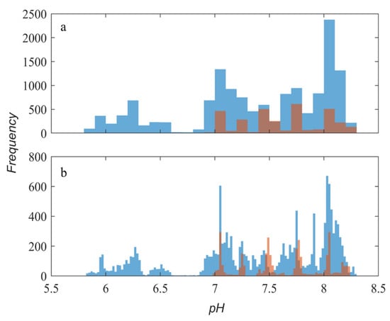
Figure 7.
Histograms of Datasets 1 and 2 with different bin width. Bin width = (a) 0.1 and (b) 0.02. Color represents orange = dataset 1 and blue = dataset 2.
Figure 8 plots the frequency density of the different histograms. The orange lines with and without markers represent the density distribution of Dataset 1 with a bin width of 0.1 and 0.02, respectively. It can be observed that their density distributions were consistent with each other in general. In addition, the blue lines from Dataset 2 showed similarity as well, and frequency densities of both bin widths were in the same order of magnitude. Thus, the results show that the effects due to frequency density and bin width are relatively independent.
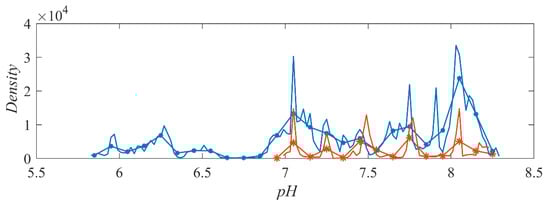
Figure 8.
Frequency density of different histograms. Color represents orange = Dataset 1 and blue = Dataset 2. Solid line without marker = bin width 0.02 and with marker = bin width 0.1.
Experiments with various frequency densities were also conducted for further investigations, and their prediction accuracies in terms of MAE are listed in Table 4. When the frequency density was higher than 1000, the performance became steady, indicating that sufficient samples were collected for the training datasets. If the density was smaller than 1000, the MAE of the predictions began to grow and increased 60% when the density decreased from 1000 to 20. As discussed above, although a higher density can potentially lead to a higher prediction accuracy, the overall performance may deteriorate due to redundant samples in the training datasets, and thus a longer training time is required. For example, a frequency density of 4000 yielded the best performance in this study according to Table 4, instead of a frequency density of 15,000.
Table 4.
Prediction accuracy with different frequency densities (number of bins = 10).
The effect due to the number of bins was also analyzed in this study, and the results are summarized in Table 5. Different bins with a frequency density of 4000 were investigated first, and the results showed no obvious difference in MAE between the predictions and observations. This can be attributed to the fact that a frequency density of 4000 was sufficient in this case regardless of the number of bins. A smaller frequency density of 100 was also examined, and the prediction accuracy was affected by the number of bins in this case. The MAE increased from 0.017 to 0.019, 0.020 and 0.021 when the number of bins decreased to 50, 10 and 2, respectively. Thus, the overall results showed that the sample distribution is more important under the circumstance of a limited training dataset, and more bins are needed to achieve a balanced dataset with a narrower sparse area.
Table 5.
MAE of predictions with different number of bins and densities.
In summary, both the frequency density and number of bins can affect the overall prediction accuracy by affecting the time needed to reload the model in the forecast updating script. The reloading records of the scenarios listed in Table 4 are tracked and further shown in Figure 9a. It is obvious that reloading was more frequent in the scenarios with a higher frequency density. In addition, with a smaller density, the reloading process tended to stop much earlier because their dataset sizes had already hit the limit. For example, the reloading records for densities of 40 and 20 only appeared before 11,000 s, while the models were continuously reloaded after 14,000 s for densities higher than 1000. Similarly, Figure 9b shows the records of the scenarios with a density of 100 in Table 5. The performance with different bins can be explained by the reloading process as well, in that a smaller MAE comes with more model updates. Thus, it can be summarized that a more frequent reloading process will eventually lead to better overall performance in the coverage-based model-updating framework.
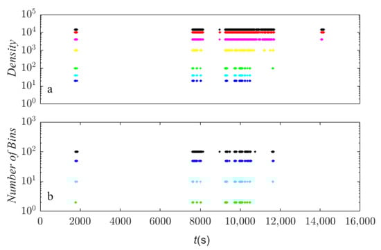
Figure 9.
Reloading records for various scenarios: (a) 10 bins with different frequency density; and (b) 100 frequency density with different number of bins. Color represents (a) black = 15,000, red = 10,000, magenta = 4000, yellow = 1000, green = 100, cyan = 40, blue = 20, and (b) black = 100, blue = 50, cyan = 10, green = 2.
5. Conclusions
In this study, a novel data-processing framework for the digital twin of water treatment facilities was proposed with real-time model updating in the process control. New coverage-based updating algorithms were developed to improve the framework performance in terms of prediction accuracy. Furthermore, the framework was comprehensively tested in the protype facility of the SWaT system under real-time operational scenarios. The overall test results show that the framework can synchronize the simultaneous forecasting and model updating, and optimized algorithms embedded in the framework can lead to a large reduction in error of up to 97%, compared to without the real-time updating. This good performance can be attributed to the coverage-based updating algorithms which control the size of training datasets with a suitable frequency density and bins to accelerate ML model updating during synchronization.
Author Contributions
Conceptualization, Y.W. and A.W.-K.L.; methodology and analysis, Y.W.; data curation, Y.W.; writing—original draft preparation, Y.W.; writing—review and editing, Y.W., A.W.-K.L.; supervision, A.W.-K.L. and C.Y.; funding acquisition, A.W.-K.L. All authors have read and agreed to the published version of the manuscript.
Funding
This research was funded by the National Research Foundation (NRF), Prime Minister’s Office, Singapore, under its National Cybersecurity R&D Program and administered by the National Satellite of Excellence in Design Science and Technology for Secure Critical Infrastructure, Award No. NSoE_DeST-SCI2019-0011.
Conflicts of Interest
The authors declare no conflict of interest.
Nomenclature
| frequency of ith bin | |
| frequency of ith bin in max area | |
| frequency of ith bin in min area | |
| density of ith bin | |
| density of ith bin in max area | |
| density of ith bin in min area | |
| threshold of frequency density in histogram selection criteria | |
| number of bins | |
| number of useful samples in the insufficient bin | |
| maximum target value in the original training dataset | |
| minimum target value in the original training dataset | |
| bin width | |
| maximum target value in the previous training dataset | |
| minimum target value in the previous training dataset | |
| maximum target value in the new training dataset | |
| minimum target value in the new training dataset |
References
- Tao, F.; Zhang, H.; Liu, A.; Nee, A.Y. Digital twin in industry: State-of-the-art. IEEE Trans. Ind. Inform. 2018, 15, 2405–2415. [Google Scholar] [CrossRef]
- Kaur, M.J.; Mishra, V.P.; Maheshwari, P. The convergence of digital twin, IoT, and machine learning: Transforming data into action. In Digital Twin Technologies and Smart Cities; Springer: Berlin/Heidelberg, Germany, 2020; pp. 3–17. [Google Scholar]
- Silva, A.J.; Cortez, P.; Pereira, C.; Pilastri, A. Business analytics in industry 4.0: A systematic review. Expert Syst. 2021, 38, e12741. [Google Scholar] [CrossRef]
- Min, Q.; Lu, Y.; Liu, Z.; Su, C.; Wang, B. Machine learning based digital twin framework for production optimization in petrochemical industry. Int. J. Inf. Manag. 2019, 49, 502–519. [Google Scholar] [CrossRef]
- Snijders, R.; Pileggi, P.; Broekhuijsen, J.; Verriet, J.; Wiering, M.; Kok, K. Machine learning for digital twins to predict responsiveness of cyber-physical energy systems. In Proceedings of the 2020 8th Workshop on Modeling and Simulation of Cyber-Physical Energy Systems, online, 21 April 2020; pp. 1–6. [Google Scholar]
- Xu, Q.; Ali, S.; Yue, T. Digital twin-based anomaly detection in cyber-physical systems. In Proceedings of the 2021 14th IEEE Conference on Software Testing, Verification and Validation (ICST), Porto de Galinhas, Brazil, 12–16 April 2021; pp. 205–216. [Google Scholar]
- Wang, J.; Ye, L.; Gao, R.X.; Li, C.; Zhang, L. Digital Twin for rotating machinery fault diagnosis in smart manufacturing. Int. J. Prod. Res. 2019, 57, 3920–3934. [Google Scholar] [CrossRef]
- Wei, Y.; Hu, T.; Zhou, T.; Ye, Y.; Luo, W. Consistency retention method for CNC machine tool digital twin model. J. Manuf. Syst. 2021, 58, 313–322. [Google Scholar] [CrossRef]
- Farhat, M.H.; Chiementin, X.; Chaari, F.; Bolaers, F.; Haddar, M. Digital twin-driven machine learning: Ball bearings fault severity classification. Meas. Sci. Technol. 2021, 32, 044006. [Google Scholar] [CrossRef]
- Adam, G.A.; Chang, C.-H.K.; Haibe-Kains, B.; Goldenberg, A. Error Amplification When Updating Deployed Machine Learning Models. In Proceedings of the Machine Learning for Healthcare Conference, Durham, NC, USA, 5–6 August 2022. [Google Scholar]
- Li, D.-C.; Chang, C.-C.; Liu, C.-W.; Chen, W.-C. A new approach for manufacturing forecast problems with insufficient data: The case of TFT–LCDs. J. Intell. Manuf. 2013, 24, 225–233. [Google Scholar] [CrossRef]
- Li, D.-C.; Wu, C.-S.; Tsai, T.-I.; Lina, Y.-S. Using mega-trend-diffusion and artificial samples in small data set learning for early flexible manufacturing system scheduling knowledge. Comput. Oper. Res. 2007, 34, 966–982. [Google Scholar] [CrossRef]
- Wei, Y.; Law, A.W.-K.; Yang, C.; Tang, D. Combined Anomaly Detection Framework for Digital Twins of Water Treatment Facilities. Water 2022, 14, 1001. [Google Scholar] [CrossRef]
- Qi, D.; Majda, A.J. Using machine learning to predict extreme events in complex systems. Proc. Natl. Acad. Sci. USA 2020, 117, 52–59. [Google Scholar] [CrossRef]
- Gepperth, A.; Hammer, B. Incremental learning algorithms and applications. In Proceedings of the European Symposium on Artificial Neural Networks (ESANN), Bruges, Belgium, 27–29 April 2016. [Google Scholar]
- Castro, F.M.; Marín-Jiménez, M.J.; Guil, N.; Schmid, C.; Alahari, K. End-to-end incremental learning. In Proceedings of the European Conference on Computer Vision (ECCV), Munich, Germany, 8–14 September 2018. [Google Scholar]
- Rebuffi, S.-A.; Kolesnikov, A.; Sperl, G.; Lampert, C.H. icarl: Incremental classifier and representation learning. In Proceedings of the IEEE Conference on Computer Vision and Pattern Recognition, Honolulu, HI, USA, 21–26 July 2017. [Google Scholar]
- Wu, Y.; Chen, Y.; Wang, L.; Ye, Y.; Liu, Z.; Guo, Y.; Fu, Y. Large scale incremental learning. In Proceedings of the IEEE/CVF Conference on Computer Vision and Pattern Recognition, Long Beach, CA, USA, 15–20 June 2019. [Google Scholar]
- Chen, T.; Guestrin, C. Xgboost: A scalable tree boosting system. In Proceedings of the 22nd ACM SIGKDD International Conference on Knowledge Discovery and Data Mining, San Francisco, CA, USA, 13–17 August 2016. [Google Scholar]
- Tarasenko, A. Is It Possible to Update a Model with New Data without Retraining the Model from Scratch? Available online: https://github.com/dmlc/xgboost/issues/3055#issuecomment-359648107 (accessed on 1 September 2022).
- Zhang, P.; Zhou, C.; Wang, P.; Gao, B.J.; Zhu, X.; Guo, L. E-Tree: An Efficient Indexing Structure for Ensemble Models on Data Streams. IEEE Trans. Knowl. Data Eng. 2015, 27, 461–474. [Google Scholar] [CrossRef]
- Guajardo, J.A.; Weber, R.; Miranda, J. A model updating strategy for predicting time series with seasonal patterns. Appl. Soft Comput. 2010, 10, 276–283. [Google Scholar] [CrossRef]
- Liu, Q.; Hu, X.; Ye, M.; Cheng, X.; Li, F. Gas recognition under sensor drift by using deep learning. Int. J. Intell. Syst. 2015, 30, 907–922. [Google Scholar] [CrossRef]
- Wang, X.; Fan, Y.; Huang, Y.; Ling, J.; Klimowicz, A.; Pagano, G.; Li, B. Solving Sensor Reading Drifting Using Denoising Data Processing Algorithm (DDPA) for Long-Term Continuous and Accurate Monitoring of Ammonium in Wastewater. ACS EST Water 2020, 1, 530–541. [Google Scholar] [CrossRef]
- Leigh, C.; Alsibai, O.; Hyndman, R.J.; Kandanaarachchi, S.; King, O.C.; McGree, J.M.; Neelamraju, C.; Strauss, J.; Talagala, P.D.; Turner, R.D. A framework for automated anomaly detection in high frequency water-quality data from in situ sensors. Sci. Total Environ. 2019, 664, 885–898. [Google Scholar] [CrossRef]
- Maag, B.; Zhou, Z.; Thiele, L. A survey on sensor calibration in air pollution monitoring deployments. IEEE Internet Things J. 2018, 5, 4857–4870. [Google Scholar] [CrossRef]
- Malinin, A.; Prokhorenkova, L.; Ustimenko, A. Uncertainty in Gradient Boosting via Ensembles. In Proceedings of the International Conference on Learning Representations, Online, 3–7 May 2021. [Google Scholar]
- Yang, Y.; Che, J.; Li, Y.; Zhao, Y.; Zhu, S. An incremental electric load forecasting model based on support vector regression. Energy 2016, 113, 796–808. [Google Scholar] [CrossRef]
- Mathur, A.P.; Tippenhauer, N.O. SWaT: A water treatment testbed for research and training on ICS security. In Proceedings of the 2016 International Workshop on Cyber-Physical Systems for Smart Water Networks (CySWater), Vienna, Austria, 11 April 2016. [Google Scholar]
- Raman, M.G.; Dong, W.; Mathur, A. Deep autoencoders as anomaly detectors: Method and case study in a distributed water treatment plant. Comput. Secur. 2020, 99, 102055. [Google Scholar] [CrossRef]
- Wang, D.; Thunéll, S.; Lindberg, U.; Jiang, L.; Trygg, J.; Tysklind, M.; Souihi, N. A machine learning framework to improve effluent quality control in wastewater treatment plants. Sci. Total Environ. 2021, 784, 147138. [Google Scholar] [CrossRef]
- Li, L.; Rong, S.; Wang, R.; Yu, S. Recent advances in artificial intelligence and machine learning for nonlinear relationship analysis and process control in drinking water treatment: A review. Chem. Eng. J. 2021, 405, 126673. [Google Scholar] [CrossRef]
- Al Aani, S.; Bonny, T.; Hasan, S.W.; Hilal, N. Can machine language and artificial intelligence revolutionize process automation for water treatment and desalination? Desalination 2019, 458, 84–96. [Google Scholar] [CrossRef]
- Newhart, K.B.; Goldman-Torres, J.E.; Freedman, D.E.; Wisdom, K.B.; Hering, A.S.; Cath, T.Y. Prediction of peracetic acid disinfection performance for secondary municipal wastewater treatment using artificial neural networks. ACS EST Water 2020, 1, 328–338. [Google Scholar] [CrossRef]
- Duan, T.; Anand, A.; Ding, D.Y.; Thai, K.K.; Basu, S.; Ng, A.; Schuler, A. Ngboost: Natural gradient boosting for probabilistic prediction. In Proceedings of the International Conference on Machine Learning, Online, 13–18 July 2020; pp. 2690–2700. [Google Scholar]
- Salcedo-Sanz, S.; Cornejo-Bueno, L.; Prieto, L.; Paredes, D.; García-Herrera, R. Feature selection in machine learning prediction systems for renewable energy applications. Renew. Sustain. Energy Rev. 2018, 90, 728–741. [Google Scholar] [CrossRef]
- Liashchynskyi, P.; Liashchynskyi, P. Grid search, random search, genetic algorithm: A big comparison for nas. arXiv 2019, arXiv:1912.06059. [Google Scholar]


Publisher’s Note: MDPI stays neutral with regard to jurisdictional claims in published maps and institutional affiliations. |
© 2022 by the authors. Licensee MDPI, Basel, Switzerland. This article is an open access article distributed under the terms and conditions of the Creative Commons Attribution (CC BY) license (https://creativecommons.org/licenses/by/4.0/).