Seasonal Variability of the Dynamics and Energy Transport in the Black Sea by Simulation Data

Abstract

This paper presents an assessment of the seasonal variability of the velocity fields, mean and eddy kinetics, and available potential energies, and the energy conversion rates for the eddy and basin-scale circulation regimes. The data were obtained through the numerical modeling of the Black Sea circulation for 2011 and 2016. It revealed significant differences in the current structure in the southern and central sea parts for 2011 and 2016. In 2011, the Rim Current was an almost continuous cyclonic basin-scale gyre, while in 2016 a system of mesoscale anticyclones was observed in the southern part. The variability of the mean kinetic energy depends more on the circulation regime than on the season of the year, while the distribution of the mean available potential energy is predominantly seasonal. The eddy kinetic energy depends on both the circulation regime and the season. In winter, the energy transport from the mean current via a barotropic instability mechanism sustains the mesoscale eddy generation. In summer, the mesoscale variability in the basin-scale regime is provided by commensurate contributions of barotropic and baroclinic instability, and, in the eddy regime, mainly by the energy transport from the available potential energy through the baroclinic instability.

1. Introduction

The movement of water and air masses is accompanied by the transformation of energy in the system because of the barotropic and baroclinic instability of currents [1]. A collaborative analysis of the regularities of circulation structure variability and the kinetic and potential energy budgets makes it possible to detect the most significant physical processes and to assess their influence on the fluxes of matter and energy in different spatial-temporal scales. The study of the mechanisms of circulation variability based on the analysis of energy budget components has been widely used since the middle of the 20th century, starting with the works of Lorenz for the atmosphere [2], and Holland and Lin for the ocean [3]. The concept presented in [2,3] operates with such definitions as mean and eddy energies, characterizing some time-mean circulation and a time-varying deviation from this mean state, respectively. In this approach, the total energy is determined by four components: mean and eddy kinetic energies (MKE and EKE, respectively), and mean and eddy available potential energies (MPE and EPE, respectively). According to the Lorenz methodology, the general estimates of all components of the energy cycle for the global atmosphere and ocean are given in [4,5], respectively. Oceanologists use this method to investigate separate components of the energy cycle both on global [6,7] and regional [8] spatial scales. The special interest of researchers is focused on EKE and the mechanisms of its variability [9,10,11,12,13], since this component of the energy cycle characterizes the mesoscale dynamics in the ocean.

The Black Sea is a unique semi-enclosed basin, where water exchange with the world ocean is limited by the narrow Bosporus Strait. The geographical features of the sea include the relatively narrow shelf zone and the steep continental slope. The maximum sea depth is 2210 m. The Northwest Shelf (NWS) is considered a shallow zone with a depth of 5–50 m and occupies about 16% of the sea area. The map of the sea bottom topography is shown in Figure 1 with the names of the main geographical points mentioned in the paper.

Numerous studies and satellite data confirm the essential mesoscale nature of the Black Sea circulation. Work to investigate the mesoscale dynamics here was started by Blatov [14], Stanev [15,16], Oguz [17], Knysh [18], Enriquez [19], etc. In addition to the structure of the current fields and thermohaline characteristics, the authors also considered the formation mechanisms of mesoscale eddies, including the analysis of the energy in the basin. The motivation of recent numerical studies of the Black Sea lies primarily in the need to improve the accuracy of the sea forecasts—for example [20,21], to assess the impact of climate change on its main characteristics [22,23], and to study small-scale (less than 1 km) dynamics [24,25].

According to the definition introduced in [26], which is confirmed by studies [14,15,16,17,18,19], the Black Sea circulation can be represented by two types:

• Basin-scale circulation (“gyre type” in [26]) is a regime when the entire basin is covered by the cyclonic Main Black Sea Current (the Rim Current), which spreads over the continental slope;
• Eddy circulation (“sub-basin type” in [26]) is a regime when the Rim Current is partially or completely destroyed and intense mesoscale eddies evolve in the abyssal part of the sea.

Independently of the circulation regime, the structure of the Lorenz energy cycle obtained by the authors in [27] for the Black Sea differs from the world ocean one [5] because of the geographical isolation of the basin and the strong seasonal variability of atmospheric conditions. In particular, the integral energy flux, formed as a result of the conversion between MKE and MPE, is directed from MPE to MKE (in contrast to [5]), and is also confirmed by our results on the energy analysis of the Black Sea climatic current fields [28]. A number of works addressed the assessment of the influence of atmospheric condition variability on the Black Sea circulation structure and its energy characteristics, where both the modeling results [15,16,17,18,29,30,31] and the observation data [29,32] were presented.

The analysis of long-term data series shows that because of climate change in recent decades, the circulation pattern in the Black Sea has also changed: such trends as an increase in the temperature of the cold intermediate layer [33], the rise of sea level [34], enhancement of the Rim Current, and mesoscale anticyclones [22] are observed. The energy budget study can help in identifying the main physical processes determining the changes of circulation and in understanding the reasons and consequences of the observed trends. The circulation regime and the season of the year form the contribution ratio of internal and external forces to the energy budget. Therefore, the seasonal variability of the mechanisms of generation and evolution of the current field for different quasi-stable circulation regimes is of interest. Thus, the aim of this work is to study the common features and/or differences in the seasonal variability of the energy cycle components and the rates of energy conversion depending on the circulation regime. This paper continues our studies of the Black Sea energy [27,35], applying the numerical analysis of the kinetic and potential energy budget equations [28], the main construction principle of which was in exact correspondence to the finite-difference formulation of the model equations. We found that wind forcing, buoyancy fluxes, and friction are the main factors determining variations in the total energy of the Black Sea. Due to the fact that in [28] the components of the energy budget equations are calculated simultaneously with thermohydrodynamical fields, it is difficult to directly assess the eddy energy transport associated with the deviation from the mean motion. Therefore, here we use the Lorenz methodology [2] in relation to the results of the numerical modeling of the Black Sea circulation.

Section 2 describes the circulation model, numerical experiments, and formulae for the calculation of the energy characteristics. Simulation results of the Black Sea currents, the numerical assessments of the spatial-temporal variability of the energy components, and conversion rates are presented in Section 3. Features of the seasonal variability of the EKE, and the barotropic and baroclinic instability contributions are considered in Section 3.3. The interpretation of the results and the relationship between energy, forcing, and thermohaline characteristics are discussed in Section 4. The main conclusions are summarized in Section 5. Validation of the simulation data is shown in the Supplementary Materials.

2. Materials and Methods

The Black Sea simulation is carried out by using the eddy-resolving z-model of the Marine Hydrophysical Institute of the Russian Academy of Sciences, Sevastopol, Russia (MHI-model) developed by the authors [18,35,36,37]. The MHI-model is based on the Navier-Stokes equations in the Boussinesq, hydrostatics, and seawater incompressibility approximations in a Cartesian coordinate system (the x axis is directed to the east, the y axis is to the north, and the z axis is downward from the surface to the bottom). The state equation is a nonlinear function of temperature and salinity. Sea surface height is calculated from the linear kinematic surface conditions, taking into account the mass flux (the precipitation minus evaporation) from the atmosphere. The boundary conditions on the free surface also set the horizontal momentum exchange (wind stress) and the heat flux between the atmosphere and the sea. The horizontal turbulent viscosity and diffusion are approximated by a biharmonic Laplace operator with constant coefficients [37]; the vertical turbulent mixing is parameterized by the Level 2.5 Mellor-Yamada closure model [38]. In the framework of this parametrization, the model equations are supplemented with two differential equations of the kinetic energy of turbulence and the macroscale of turbulence, on the basis of which the coefficients of vertical viscosity and diffusion are calculated ([35], Equations (17)–(25)). The MHI-model configuration takes into account the monthly climatic runoff of the Dnieper, Danube, Dniester, Sakarya, Kizilirmak, Yeshilirmak, and Rioni rivers, and the exchange through the Bosporus and Kerch straits [39]. The lateral boundary conditions are free-slip for solid boundaries, and the Dirichlet condition for liquid ones. The sea level, temperature, salinity, and horizontal velocity are set at an initial moment. The main numerical methods used in the MHI-model are the following: the finite-difference approximation of the model equations is implemented on a C-grid [40]; time stepping is the Leap Frog scheme [41]; a TVD-scheme [42] is used for advective terms in salt and heat equations; the tridiagonal matrix algorithm [43] is used on vertical coordinate in momentum, heat, and salt equations; and the successive over-relaxation method [44] is used to solve the sea level equation. The complete MHImodel formulation and the features of its numerical realization are presented in detail in [35,36]. The MHI-model was tested and validated in the European Union’s ARENA, ASCABOS, ECOOP, and MyOcean framework projects. The model demonstrated a high level of agreement between reconstructed hydrophysical fields and observation data [45,46]. The limitations of the MHI-model are in the following assumptions. The model was constructed in a hydrostatic approximation using linearized conditions on the free surface and climatic flows in rivers and straits. The mass balance in the model is maintained by the inflow with the lower Bosporus current, which is calculated based on the balance of water coming from the atmosphere plus the climatic inflow of rivers plus the outflow with the upper Bosporus current. The SST is assimilated in the model to reduce the error in calculating the local density in the upper sea layer caused by the inaccuracy of atmospheric heat fluxes. The MHI-model does not take into account the tidal forcing, since the tidal fluctuations in the Black Sea do not exceed 17 cm (according to observational and modeling data [47]) because of the narrowness of the Bosporus Strait and the relatively large sea surface area of 422,000 km².

The Black Sea model domain is a uniform grid with a horizontal resolution of (1/48)° longitude and (1/66)° latitude, which is equal to about 1.6 km in the area between 27.34–41.9 E and 40.86–46.56 N. The model domain bathymetry is built on the data of the European Marine Observation and Data Network (EMODnet, http://portal.emodnet-bathymetry.eu, accessed on 24 November 2021) with the resolution of (1/8)′. The vertical resolution is 27 horizons with depths of 2.5, 5, 10, 15, 20, 25, 30, 40, 50, 62.5, 75, 87.5, 100, 112.5, 150, and 200 m, from 200 till 500 m every 100 m, and from 700 till 2100 m every 200 m. Also note that the horizontal grid step used is much smaller than the baroclinic Rossby deformation radius (10–30 km according to observations [48]), so physical eddies are explicitly resolved in the model. It was confirmed in [27,37], where model current maps were compared with satellite images, and it was shown that the main mesoscale eddies in the simulated velocity field qualitatively correspond to the real pattern of currents. The influence of the spatial grid step size was evaluated by comparing the simulated results of the Black Sea circulation with a resolution of 5 km and 1.6 km [35]. We found that with an increase in the model resolution the current structure was barely changed qualitatively since mesoscale eddies were resolved explicitly, but the energy and phase characteristics were changed quantitatively.

The circulation is driven by realistic 6-h forcing (including wind velocity, thermal, latent, sensible, and solar heat fluxes, evaporation, precipitation, and sea surface temperature SST), which is provided by the SKIRON/Dust modeling system with the spatial resolution of 0.1° [49]. In the text we refer to it as SKIRON data. Numerical experiments started from the initial fields constructed on the CMEMS reanalysis data for the Black Sea [50]. The CMEMS reanalysis is forced by ERA-5.Therefore, we use a quasi-geostrophic adjustment procedure [36] to reconcile the hydrophysical and atmospheric fields at a preliminary stage. The model output is of daily fields of sea level, temperature, salinity, and current velocities.

The energy analysis is carried out for two time intervals (2011 and 2016), when the mean Black Sea circulation corresponded to the regimes described in [26]. Maps of the annual mean surface currents velocity for 2011 and 2016 are shown in Figure 2. It can be seen that the basin-scale circulation regime with the Rim Current covering the entire sea was realized in 2011 (Figure 2a). The eddy regime with mesoscale eddies prevailing in the central sea part was observed in 2016 (Figure 2b). The structure and description of the hydrophysical fields and comparison with in situ data are given in [27,37]. Some validation results are also presented in Tables S1 and S2, and in Figure S1 of the Supplementary Materials.

According to [3,5], the ocean energy cycle is formed by four main components—MKE, EKE, MPE, and EPE. External conditions (such as wind, fluxes of heat, and freshwater) are the sources of energy, the decrease in energy occurs because of dissipation and diffusion. The energy transport from MKE to EKE took place through the mechanism of barotropic instability (denote BT) caused by a shift in the current velocity. If the change in the current velocity is due to the increase in slope of the isopycnal planes, then the energy conversion occurs from MPE via EPE to EKE through the mechanism of baroclinic instability (denote BC). A preliminary analysis of the simulation results shows that the zones of MPE→EPE transport qualitatively and quantitatively correspond to the zones of EPE→EKE transport. Therefore, in this work, we consider the MPE→EPE transport to estimate the BC in the Black Sea. Note that this energy flux is a measure of baroclinic production. The exchange between MPE and MKE is provided by the buoyancy work (denote BW). As it is known, one of the main factors determining the Black Sea circulation regime is wind forcing [17,29,30,51]. Analysis of the annual mean components of the Lorentz energy cycle for 2011 and 2016 [52] shows that our results agree with this concept. In addition, we found that the energy transport caused by barotropic and baroclinic instability can be commensurate with the contribution of the wind stress work under a weakening of the wind forcing. Therefore, in this work we focus on studying the energy conversion caused by the buoyancy work and instability processes.

To analyze the mechanisms of the spatial-temporal variability of the energy cycle components, the parameters MKE, EKE, MPE, EPE, BT, BC, and BW are calculated using the MHI-simulation data on the current velocity (u, v, w) and seawater density (ρ). Following [5,10], the energy parameters can be written as:

$$\begin{gathered} MKE=\frac{1}{2}{\rho }_0\left({\overline{u}}^2+{\overline{v}}^2\right), EKE=\frac{1}{2}{\rho }_0\overline{\left({u^{\prime }}^2+{v^{\prime }}^2\right)}, \\ MPE=\frac{1}{2}g{\left(\frac{\partial \langle \overline{\rho }\rangle }{\partial z}\right)}^{-1}{\overline{{\rho }^{*}}}^2, EPE=\frac{1}{2}g{\left(\frac{\partial \langle \overline{\rho }\rangle }{\partial z}\right)}^{-1}\overline{{\rho }^{{*}^{\prime }}{}^2}, \\ BT=-{\rho }_0\left[\overline{{u^{\prime }}^2}\frac{\partial \overline{u}}{\partial x}+\overline{{v^{\prime }}^2}\frac{\partial \overline{v}}{\partial y}+\overline{u^{\prime }{v}^{\prime }}\left(\frac{\partial \overline{v}}{\partial x}+\frac{\partial \overline{u}}{\partial y}\right)\right], {\rho }^{*}=\rho -{\rho }_{ref}\left(z\right), \\ BC=g{\left(\frac{\partial \langle \overline{\rho }\rangle }{\partial z}\right)}^{-1}\left(\overline{u^{\prime }{\rho }^{*\prime }}\frac{\partial \overline{{\rho }^{*}}}{\partial x}+\overline{v^{\prime }{\rho }^{*’}}\frac{\partial \overline{{\rho }^{*}}}{\partial y}\right), BW=g\overline{{\rho }^{*}}\overline{w}, \end{gathered}$$

(1)

where g is the gravity acceleration, ρ_ref is the reference density, and ρ₀ = 1000 kg/m³. The overbar denotes time averaging, the prime denotes the deviation from the mean value, and angle brackets denote area averaging. Also note that the z axis is directed downward in the MHI-model, so the square of the Brunt-Vaisala frequency is N² > 0 ($N^2=\frac{g}{\rho }\frac{\partial \rho }{\partial z}$). The parameter ρ_ref is calculated as the average area density for the corresponding horizon; it is a constant for each model layer. It is known that the typical lifetime of the main mesoscale eddies in the Black Sea varies from 3 (for example, the Sevastopol Eddy) to 9 months (the Batumi Eddy) [39]. In this work, the time-averaging interval is one month, which allows us to estimate seasonal variations in the energy fluxes without smoothing the mesoscale structure of the current field. Later in the text, we consider the hydrological seasons of the year: winter is from January–March, spring is April–June, summer is July–September, and autumn is October–December.

3. Results

3.1. Seasonal Variability of the Velocity Field

Let us consider the seasonal variability of the Black Sea circulation structure according to the MHI-simulation data in 2011 and 2016. Current velocity fields averaged over each hydrological season are analyzed on 5, 30, 50, 100, and 200 m horizons. As an example, Figure 3 shows currents velocity maps on the 5 m horizon for each season.

In winter (Figure 3a) and spring (Figure 3b) of 2011, the Rim Current is a strong narrow jet located above the continental slope. The Rim Current is practically continuous, excluding the eastern part of the basin, and is found in a 0–200 m layer. In summer, the current is broken near the Caucasian coast (Figure 3c), and there is a weakening and meandering of the Rim Current at the border of the NWS. In autumn, an extensive meander in the central part of the basin near the Anatolian coast (Figure 3d) practically divides the Rim Current into western and eastern cyclonic gyres, which are detected to a depth of 100 m. An anticyclonic gyre is formed from the indicated meander at 200 m deep. The Rim Current is the most intense in spring on the considered horizons, especially in the western part of the basin. The maximum velocities during this period reach 30–33 cm/s in a 5–30 m layer, while in other seasons they do not exceed 24–27 cm/s. The maximum velocities on 200 m vary insignificantly throughout the year and do not exceed 16–17 cm/s.

An anticyclonic eddy between the Rim Current and the coast near Trabzon, Turkey is observed in winter. In spring, the Batumi Eddy is formed from this anticyclone. The Batumi Eddy achieves its maximum diameter in summer, and has maximum velocities up to 27 cm/s on 5 m in autumn. The Batumi Eddy moved westward by about 1° E during spring–autumn 2011.

In winter 2016, the Rim Current is located on periphery of the deep-water part, excluding the area near the Anatolian coast westward of Trabzon, Turkey (Figure 3e). The maximum velocities in the upper 50-m layer are detected along the Caucasian coast, where the velocity varies from 30–33 cm/s in the subsurface layer to 21–24 cm/s at 50 m. On the 100 and 200 m horizons, the maximum velocities are observed near the Crimean coast and reach 16–18 cm/s and 10–11 cm/s, respectively. In the abyssal eastern part of the basin, an anticyclonic eddy with a diameter of about 250 km is traced in the upper 0–200 m layer. The eddy size slightly decreases with the depth; the maximum orbital velocities vary from 21–24 cm/s at 5 m to 7–8 cm/s at 200 m. In the rest of the year (spring–autumn 2016), only some elements of the Rim Current are found in different parts of the basin in the 0–200 m layer (Figure 3f–h).

In spring, a chain of mesoscale anticyclones is formed near the Anatolian coast. From spring to summer, this chain evolves into a system of eddies of different vorticity signs in the southeastern part. These eddies reach the highest intensity in summer; their sizes vary from 50 to 150 km. The maximum orbital velocities reach 24–27 cm/s in the 0–50 m layer and decrease to 10 cm/s at 200 m.

A comparison of the model velocity fields and the satellite images of sea surface temperature and chlorophyll A distribution confirms the correspondence of the simulation data and the realistic pattern of the currents. Examples are shown in Figure S1 of the Supplementary Materials.

3.2. Seasonal Variability of Energy Characteristics

Using formulas (1), we calculated the monthly spatial distributions of the energy cycle components for two circulation regimes. To assess the seasonal variability of the energy characteristics, these parameters were averaged over each model layer, and the dependences of its area-mean values on depth and time were constructed. Let us consider the variability of MKE and MPE, the energy exchange between of them takes place because of the buoyancy work BW. Figure 4 shows the seasonal changes of MKE, MPE, and BW per unit volume for 2011 and 2016. A positive value of BW corresponds to the MPE→MKE conversion.

The weakening of the MKE in spring–summer, typical of the basin-scale circulation, is observed in 2011. The maximum energy of the mean current is revealed in April, which corresponds to the intensification of the Rim Current in spring (Figure 3b). The most energetically active layer in terms of MKE lies in the depths from 0 to 70 m in April–May and October–November 2011. The seasonal signal in the MPE variability is manifested as an increase in energy from June till October (Figure 4a, MPE diagram), which is associated with the influence of the heat fluxes on the Black Sea’s surface. As can be seen from Figure 4a, areas of increased MPE values are traced up to 20 m, which corresponds to the depth of the upper boundary of the seasonal thermocline. The relationship of the spatial distribution of MPE with the thermohaline characteristics of seawater and fluxes from the atmosphere are demonstrated in Section 4. The BW increased the MKE in the upper 10–20 m layer during the year, and below 40 m in the summer of 2011. The BW is negative throughout the year in the layer 20–40 m deep, which indicates the transport of MKE→MPE.

Let us consider the seasonal variability of the parameters MKE, MPE, and BW in 2016 (Figure 4b). Increased MKE values were observed in January and February in the upper 30-m layer; the MKE reserve is minimal from March–June. By the end of the year, the northern branch of the Rim Current appeared in the velocity field (Figure 3h), which leads to a insignificant increase in the MKE. The seasonal variability of the MPE does not correlate with the change in the kinetic energy; its increased values were observed from June to September in the upper 20-m layer. The BW in the upper 20 m layer is positive throughout the year, hence MPE is converted to MKE. Since spring 2016, the area of positive BW values has also been observed at depths below 40 m, herewith from March till July (when the size of this area is the greatest) increased values in MKE distribution are also observed on horizons of 50–70 m.

The variability of the EKE is determined by the contributions of the barotropic and baroclinic instability processes. Positive values of BT correspond to the МКЕ→ЕКЕ conversion, and positive values of BC correspond to the МРЕ→ЕРЕ transformation. The seasonal variation of the ЕКЕ, ВТ, and ВС per unit volume for 2011 and 2016 are shown in Figure 5.

In 2011 (the basin-scale circulation regime), increased EKE values were observed from April till October, and the main EKE reserve was concentrated in the 0–60 m layer (Figure 5a). The main contribution to the EKE value at this time was made primarily by the Batumi and Sevastopol Eddies forming in the southeastern part of the sea and westward of Sevastopol, Russia, respectively (Figure 3b,c). The intensification of mesoscale variability in the warm period is associated with the Rim Current weakening as a result of a decrease in the wind vorticity [17,30]. Throughout the year, the BT value was positive in the upper near-surface layer, which is related to the wind effect on the upper sea layer, where maximum current velocities generate shear instability leading to energy transport from the MKE to the EKE. In summer 2011, extensive areas of negative BT values were observed in the upper 100-m layer, which leads to a decrease in the EKE reserve compared to the spring values. Apparently, in the summer season when the wind effect weakens and the energy inflow from the wind is significant only in the upper sea layer, the horizontal velocity gradients are caused by the complex thermohaline circulation. This is merely our hypothesis, the confirmation or refutation of which requires a separate study. The BC is negative in the cold season and positive in the upper 40-m layer in spring and summer. An increase in baroclinic production here is associated with a seasonal increase in vertical density gradients. Thus, in the cold period of 2011, the contribution of BT prevailed in the budget of the EKE, and, in the warm period, the contributions of BT and BC were comparable in magnitude. It should be noted that instability in the EKE budget is energetically significant against the background of the mutual compensation of the fluxes from wind and energy dissipation.

In 2016 (Figure 5b), the ratio of the BT and BC contributions and the seasonal variability of EKE are different from in 2011. First, the maximum values of the EKE are observed in winter and autumn, in contrast to in the spring and summer in 2011. As can be seen from Figure 5b, the increased EKE values in winter and autumn 2016 correspond to the maximum BT contribution in the upper 100-m layer. However, from April till September, the BT value is negative in the entire layer; i.e., the energy flux is directed from the eddies to the mean current, and, on the contrary, the BC is positive. Consequently, in the warm period of 2016, the energy flux to the EKE is induced mainly by baroclinic instability.

3.3. Intensification Mechanisms of Mesoscale Variability

Usually, EKE in the ocean is associated with mesoscale variability. The Rossby’s baroclinic radius of deformation in the Black Sea is, on average, from 10 to 30 km [48]; therefore, we consider eddies with sizes of 30–100 km as mesoscale. The above-described peculiarities of the seasonal variability of energy fluxes can be supplemented by an analysis of the spatial distribution of the energy budget components and their comparison with the zones of mesoscale eddies intensification.

Figure 6 and Figure 7 show the spatial distribution maps of EKE, BT, and BC for 2011 and 2016 in February and August, as they are the most characteristic months of the cold and warm seasons. The 2D arrays of EKE, BT, and BC per unit area are obtained by vertical integration of the three-dimensional fields EKE, BT, and BC in the layer from 0 to 200 m.

According to the calculations, we found that in February 2011 (Figure 6a) increased EKE values are observed only at the periphery of the Rim Current in the southern part of the sea. This is an energy-active zone, where eddies with sizes of 30–40 km in diameter form almost continuously. The BT modulus is maximal here because of the bottom topography and the significant shear of the current velocity on the roughness of the coast.

In winter 2016 (Figure 6b) the structure of the EKE field is significantly different: this parameter above the continental slope is two to three times larger compared to 2011. Areas of the highest EKE values (more than 7 J/m²) are located to the southwest of the Crimea and northeast of the Bosporus. In both zones, the increase in EKE occurs because of the conversion of energy from the mean current. In February 2016, two gyres were also clearly distinguished in the eastern part of the sea, and if the eddy near the Crimean coast is associated with the intensification of the baroclinic instability (increased values of BC), then the gyre in the southeastern part corresponds to the zone of barotropic instability (increased values of BT).

In summer, the weakening of the Rim Current and the intensification of eddy variability are observed in the Black Sea. The simulation results show that the maximum EKE was reached in the Sevastopol Eddy zone in August 2011 (Figure 7a). An intense energy exchange takes place here between the mean current and eddy structures: the inhomogeneity of the extreme BT values indicates this. Also, the flux from the EPE makes significant contributions to EKE, which corresponds to the zones of maximum BC values. The contributions of the BC and BT to the energy of the Sevastopol Eddy in August 2011 were comparable in magnitude to each other; the same ratio of contributions is detected near the coast of Turkey. The Batumi Eddy in August 2011 evolved because of the mean current energy.

In August 2016 (Figure 7b), the energy of eddy structures developing in the deep-water part of the sea was mainly determined by the processes of baroclinic instability. The zones of increased BC values are well in agreement with the distribution of increased EKE values, while there is no correspondence with BT.

4. Discussion

In the present work, we study the spatial-temporal variability of the mean and eddy energy, and the rates of their conversion to assess the contributions of various physical processes to the Black Sea circulation energy on a seasonal scale based on the MHI-simulation results for two full-year periods. We focus on 2011 and 2016 since the field structures of the annual mean current velocity in these time intervals correspond to the basin-scale (2011) and eddy (2016) circulation regimes in the Black Sea [26].

We obtained the results that the northern branch of the Rim Current is generated in the cold season for both regimes. The dynamics in the southern and central parts of the basin are significantly different. So, in winter, spring, and autumn 2011 the Rim Current was an almost continuous gyre, excluding the eastern part, while in 2016 the circulation was represented by a system of mesoscale anticyclones in the southern part. For the eastern part, in 2011 the Batumi Eddy demonstrated the features of a quasi-stationary eddy, but in 2016 the dynamics were characterized by the eddy system of a different vorticity sign.

The following features of the seasonal variability of the mean energy are revealed. The comparison of Figure 4a,b shows that the MKE variability depends on the type of circulation to a greater extent than on seasonal changes of external conditions: the highest values are observed in spring 2011 and in winter 2016. This is associated with the circulation structure in two experiments. The Rim Current is characterized by a quasi-stable gyre in 2011 (Figure 2a), which reaches the highest intensity after the winter winds (Figure 3b). After spring 2016, the Rim Current decays into a series of mesoscale eddies (Figure 3f), the behavior of which is strongly nonstationary.

The MPE value is strictly seasonal and depends little on the circulation regime. The highest MPE values in both experiments are observed in the summer season in the upper 20 m layer, which indicates the decisive contribution of heat and mass (total precipitation rate minus evaporation rate) fluxes from the atmosphere to the MPE value. Figure 8 shows the seasonal variability of heat and mass fluxes averaged over the sea surface in 2011 and 2016. It can be seen that the total heat flux over the sea is positive from May to October (Figure 8a), and the difference between precipitation and evaporation is negative (Figure 8b). Hence, the heat flux increases the density anomaly, while the predominated evaporation decreases it.

Diagrams of the MHI-simulation seawater thermohaline characteristics (Figure 9) show that the zone of the highest MPE values from June to October (Figure 4) is determined by an increase in the density anomaly caused by the warming of seawater. It correlates weakly with changes in salinity for both circulation regimes. Despite the fact that salinity makes the main contribution to the local density of the Black Sea water [14,15,39], the density anomaly in the upper layer in summer is formed because of an increase in temperature. Therefore, the warming up of the sea surface is one of the reasons for the increase in the APE content during summer. This conclusion is also confirmed by the result that both the MPE value (Figure 4b) and the total heat flux (Figure 8a, blue line) in 2016 exceed these parameters in comparison with 2011 (Figure 4a and Figure 8a, red line).

The variability of the BW flux has common features for both regimes:

• In the spring-winter season, the buoyancy work increases the MKE;
• Throughout the year, the BW is negative in the 20–40 m layer with minimal values in autumn.

The placement depth of the largest negative BW values corresponds to the depth of the seasonal thermocline (temperature diagrams in Figure 9). Apparently, the process of destroying of the thermocline by cooling the sea surface is accompanied by an increase in the APE owing to the buoyancy work.

The differences in the spatial-temporal variability of the BW for the two regimes appear on horizons below 40 m. Here, BW is positive only in summer 2011, while in 2016 the area of positive BW values is observed from February till the end of the year. An increase in the BW below 40 m is associated with positive density anomalies in the cold intermediate layer (CIL). Comparison of Figure 4 (BW diagrams) and Figure 9 (temperature diagrams) shows that the location of the areas of maximum positive BW values coincides with the location of the CIL waters at depths of 40–60 m. Based on the above-mentioned, it can be assumed that the buoyancy work can also enhance the kinetic energy of the mean current in the upper 20 m layer, where the wind contribution plays the main role [16,17,27], and in the 40–60 m layer, where the subsurface velocity maximum of the Rim Current core [53] is associated mainly with the maximum slope of isohalines over the continental slope.

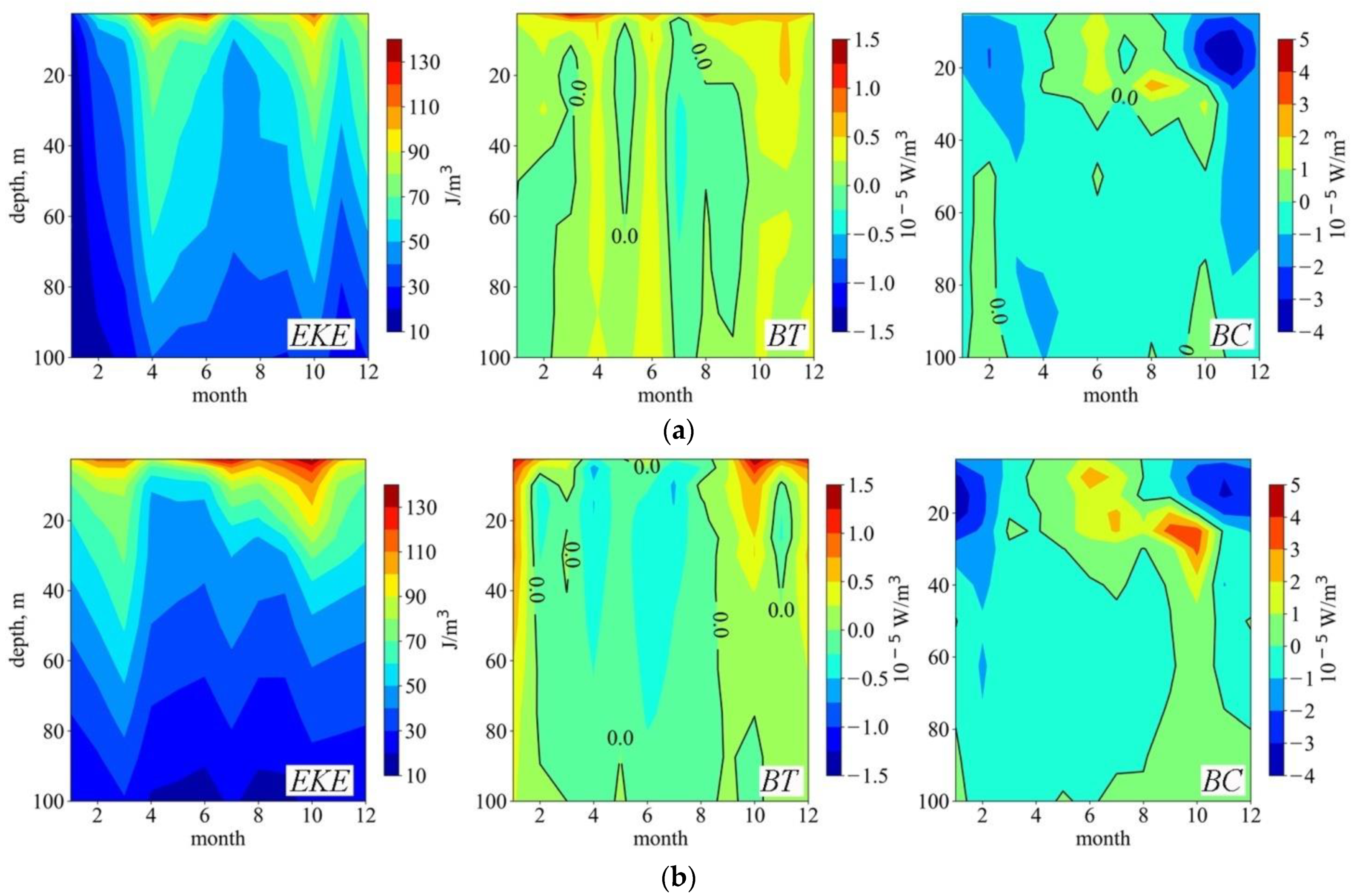
The seasonal variability of the EKE and its conversion rates caused by barotropic and baroclinic instability are analyzed. As expected, the EKE value is determined by the circulation regime. So, the maximum EKE values are observed in spring and summer 2011 (the basin-scale regime), and in winter and autumn 2016 (the eddy regime). Common features in the seasonal variability of the barotropic instability MKE→EKE for both regimes are manifested as maximum values of BT in the 0–10 m layer and predominance in the cold season. The physical explanation behind this process is the following: when the current velocities in the basin are the highest, i.e., the system has a large content of the MKE, then more energy can be converted as a result of the velocity shift. Zones of maximum BT values in Figure 5 (BT diagrams) correspond to the areas of the highest MKE values in the upper 10 m layer (Figure 4, MKE diagrams) for both experiments.

The baroclinic instability MPE→EKE is maximal in summer and is minimal in winter for both regimes. We confirm that the seasonal variability of the BC is primarily determined by the variability of the vertical density gradient. Diagrams of seasonal variability of the area-mean density gradient on the horizons are presented in Figure 10. It can be seen that the location of the zones of maximum BC values in Figure 5 corresponds to the maximum vertical density gradients. Comparing Figure 9 and Figure 10, it can be noted that the seasonal thermocline also plays a key role here. In the warm season, when the upper layer is warmed up more than the lower one—23–25 °C versus 8–8.5 °C (Figure 9)—the density gradient is maximum (Figure 10) in the thermocline layer of 20–30 m from June till September. Apparently, the value of BC (as well as MPE) through the density gradient is indirectly controlled by heat fluxes from the atmosphere since the magnitude of the gradient in 2016 (Figure 10b) and the average temperature in the upper layer (Figure 10b) are higher than in 2011. The zones of negative BC values in the upper 20 m layer in the cold season are associated with intense vertical mixing, when the density field becomes homogeneous and the BC contribution is minimal.

The main distinguishing feature is the fact that the increase in EKE in the eddy circulation regime in the spring-summer period is provided mainly by baroclinic instability. The predominance of this mechanism in spring and summer takes place because the Rim Current is divided into separate flows and gyres (Figure 3f,g), the MKE reserve is small (Figure 4b, MKE diagram), and the energy inflow from the APE makes the main contribution to the EKE budget. The spatial distribution of EKE and its conversion rates confirm the above result.

5. Conclusions

Seasonal variability of the mean and eddy kinetic energy, and the mean and eddy available potential energy, as well as the rates of their conversion, is considered for the basin-scale and the eddy Black Sea circulation regimes realized in 2011 and 2016, respectively. First, the greatest difference between 2011 and 2016 is the maximum velocities of the Rim Current elements for the identical seasons. It rises from 5 to 10 cm/s. The second important difference is the kinematics of eddies: in 2011, the most intense mesoscale eddies develop on the basin periphery above the continental slope; in 2016, such eddies are observed in the central part of the sea at depths of 1500–2000 m.

The spatial distribution of the biggest EKE values is similar for the two periods; however, quantitatively the EKE values in 2016 are two times higher than the one in 2011 in winter and 1.3 times higher in summer. For the energy conversion rates, the quantitative indicators are close in absolute values, but the spatial distribution of their contributions reflects the circulation regime. Thus, the barotropic energy transport is maximum in the Rim Current zone above the continental slope in 2011. The baroclinic energy transport is maximum in the deep part in 2016.

The seasonal signal is weakly manifested in the variability of the MKE during the year. Its value depends on the current velocities, which are higher in the basin-scale circulation regime. The distribution of the MPE is predominantly seasonal; temporal variability is qualitatively similar for both regimes and is caused by an increase in the density anomaly that is due to the warming of seawater. The energy transport MKE→MPE that is due to the buoyancy work is provided by the subsurface layer and the CIL layer.

Seasonal variability of the EKE and the mechanisms of its intensification are different for the two circulation regimes. The EKE is maximal in spring and summer in the basin-scale circulation regime, and in the cold season in the eddy circulation regime. In winter, when the Rim Current or its elements are the most intense, irrespective of the circulation regime, mesoscale eddies develop mainly because of the energy transport from the mean current via the barotropic instability mechanism. In summer, the mesoscale variability in the basin-scale circulation regime is due to the commensurate contributions of barotropic and baroclinic instability, and, in the eddy circulation regime, only to the energy transport from the MPE caused by baroclinic instability.

Let us note that the results of the present work are applicable to the deep part of the Black Sea with depths of more than 100 m. In the NWS region, the dynamics are characterized by fast submesoscale processes with a characteristic time of 1–10 days and sizes of about 1 km. Therefore, such motions are clearly not resolved by the used version of the MHI-model and it is difficult to assess their energy here. Also, these results were obtained on two relatively short time intervals and should be considered as preliminary. In the future, we plan to study the energetics of the Black Sea based on the data of long-term reanalysis. It seems logical to perform an analysis of the energy circulation for each year in a long-term period and compare the results between the average components of the energy budget with the data for some specific “extreme” years, which will make it possible to draw more general conclusions about the mechanisms of circulation variability on an interannual scale.