1. Introduction
Due to complex geological, environmental and physical effects, the parameters involved in slope stability assessments show spatial variability at multiple scales. Even in the seemingly homogeneous site for laboratory-scale sampling and measurement, the saturated hydraulic conductivity, shear strength and other parameter values of rock and soil also show great spatial variability [
1,
2,
3]. Spatial variability is an inherent property of rock and soil materials.
In recent decades, the spatial variability of rock and soil parameters has been shown by previous studies to be a factor that cannot be ignored in evaluating slope reliability. For example, Cho [
4] emphasized the importance of the spatial variability of soil mechanics parameters in the evaluation of failure probability. Ji et al. [
5] found that ignoring the spatial variability of shear strength parameters would seriously overestimate the failure probability of slopes. Griffiths et al. [
6] and Jiang et al. [
7] indicated that when the coefficient of variation of the shear strength parameter is large and the factor of safety calculated by the mean of the parameter is close to 1, ignoring the spatial variability of the shear strength parameters could lead to an unconservative estimate of the probability of slope failure. Cai et al. [
8] indicated that it is important to describe the permeability coefficient and pore water distribution in slope stability analysis using cross-correlation analysis between the factor of safety and hydraulic parameters of an infinite slope. Qi and Li [
9] studied the typical failure mechanism of the critical slip surface of a heterogeneous slope and the results show that local failure may occur in a statistically isotropic slope, which is not observed in the deterministic slope stability analysis. These studies all used probabilistic statistics methods, which allows us to describe heterogeneity of geologic formations quantitatively. Other probabilistic statistical methods, such as machine learning and artificial neural networks, also appear widely in the application of geosciences [
10,
11,
12].
Most of the aforementioned studies focused on statistically isotropic parameters. Due to large-scale geological deposition processes, slope structures are often stratified, which means that the spatial distribution of the parameters is statistically anisotropic. The statistical anisotropy of the parameters is mainly controlled by the continuity of the formation. The more continuous the formation is along the layer direction, the more obvious the statistical anisotropy of the parameters [
13]. Ye et al. [
14] conducted a hierarchical geostatistical analysis to examine the large-scale geologic structure for the entire field site and then investigated small-scale features within different layers. The ratio of horizontal to vertical spreading at varying moisture contents suggests the statistical anisotropy in effective unsaturated hydraulic conductivity, confirming existing stochastic theories. In addition, the statistical anisotropy of geotechnical materials can be obtained using remote sensing techniques [
15,
16,
17,
18,
19,
20,
21].
Therefore, it is necessary to study the effect of statistically anisotropic parameters on the probability of slope failure. In this paper, the effect of statistically anisotropic undrained shear strength on the probability of slope failure is studied. The undrained shear strength corresponds to the situation in which the geotechnical materials cannot be drained under saturated conditions. For example, the amount of infiltration into the slope during heavy rainfall is very high and it cannot be discharged in a short time. At this time, the stability of the slope is mainly determined by the undrained shear strength of the soil.
An appropriate method for calculating the probability of failure of a heterogeneous slope is the Monte Carlo simulation (MCS). MCS has been widely used in slope reliability analysis [
22,
23,
24,
25,
26,
27]. The obvious advantage of an MCS is that it increases the accuracy and reliability of the evaluation results through numerous repeated iterations. This operation can overcome the impact of data collection and human factor errors [
28]. Therefore, MCS better reflects the real phenomenon traditional reliability analysis methods. In particular, when using the finite element strength reduction method to calculate the factor of safety of slope, there is no explicit analytical solution between the geotechnical parameters and the factor of safety due to the complex non-linear relationship. Therefore, it is difficult to calculate the probability of slope failure using traditional reliability analysis methods and the use of MCS can bypass this problem.
This paper is organized as follows. First, the method for characterizing the heterogeneity of parameters is introduced and the characteristics of the distribution of statistically anisotropic undrained shear strength are illustrated. Then, the effect of the different horizontal and vertical correlation scales of undrained shear strength on the probability of slope failure is investigated by the Monte Carlo simulation. Finally, based on the analysis of the slope displacement of different correlation scales, the mechanism of the effect of the correlation scales on the probability of failure is discussed.
2. Methodology
2.1. Stochastic Conceptualization of Heterogeneity
Random field theory has become popular in recent years to describe parameter heterogeneity [
13,
29,
30]. Random field theory assumes that the parameters of each position involved in the slope stability assessment (corresponding to each element) are random variables and the whole slope becomes an ensemble of these random variables, namely, a random field. This means that there are infinite possibilities of the distributions of parameters (realizations). As we take the undrained shear strength (
cu) as a random field, it can be described by a probability density function with a specific mean, variance and autocorrelation function. The autocorrelation function represents the spatial structure of soil properties and plays a significant role in random field analysis. In practice, geotechnical materials are sampled to obtain their mechanical and hydraulic parameters. Statistical and variogram analysis of the parameter data gives the mean, variance and correlation scales under the stochastic conceptualization. In this study, to avoid negative parameter values during evaluation, an exponential 2D autocorrelation function is adopted with different correlation scales in the horizontal and vertical directions. We assume that the slope has n random variables and
i and
j = 1,2...,
n; then, the autocorrelation function can be expressed as:
where
ρij is the autocorrelation coefficient between
cu at location (
xi, yi) and at location (
xj, yj) and
λx and
λy are the horizontal and vertical correlation scales, respectively. Physically, the correlation scale describes the average dimensions (e.g., length and thickness) of heterogeneity (e.g., layers or stratifications) within the domain [
13].
When
λx is equal to
λy in a random field, it is called a statistical isotropic random field. In
Figure 1,
λx is equal to
λy, increasing successively to 0.5 m, 2 m and 5 m, respectively. This parameter field corresponds to the condition that the slope is the accumulation of a large number of spherical geological bodies (such as gravel beds or sandy soil beds), where the average gravel or sand particle radius is approximately equal to the correlation scale
λ. Certainly, each globular body can be made up of different shapes and properties, as well as the density of their distribution. The realizations are generated by a spectral method [
31].
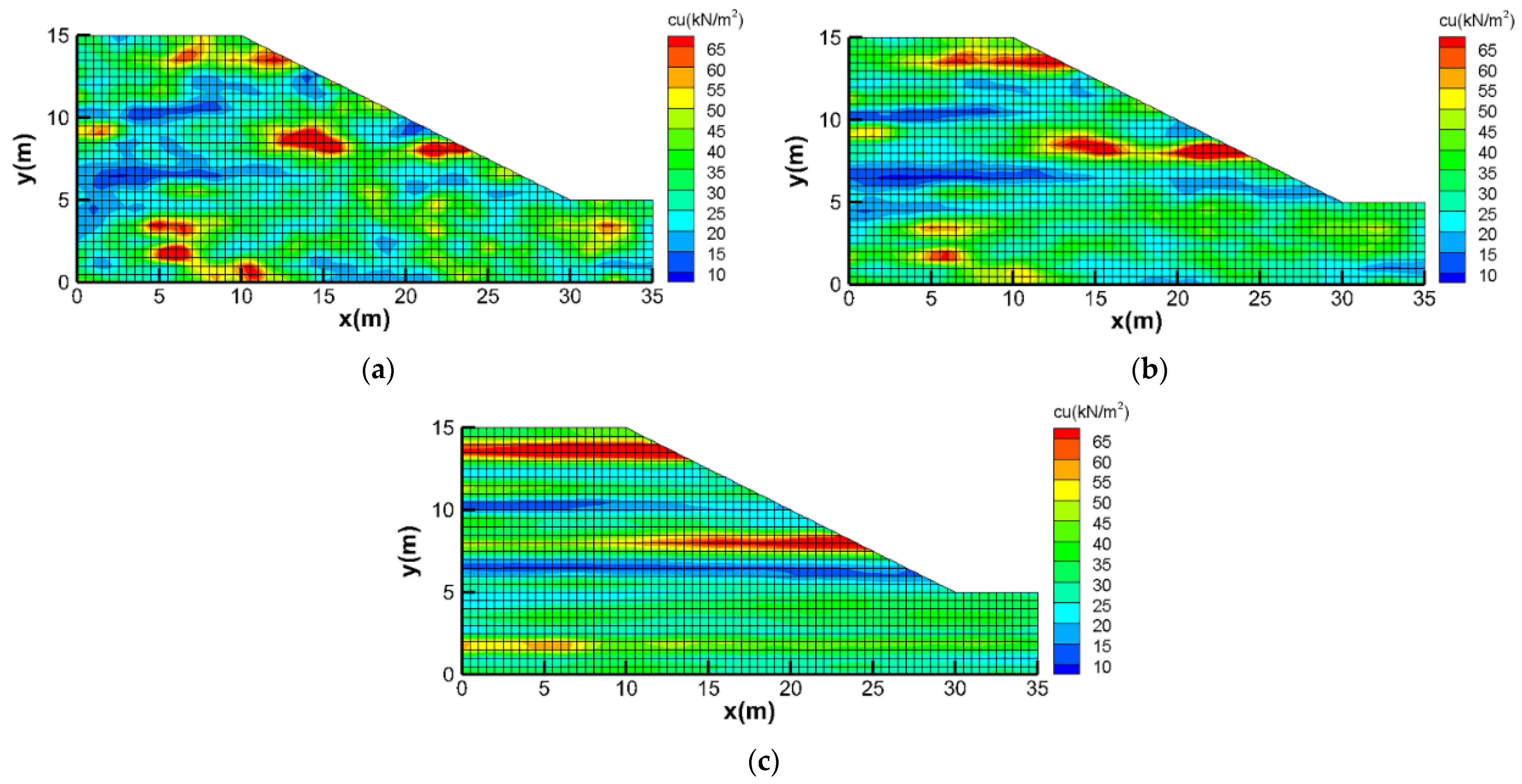
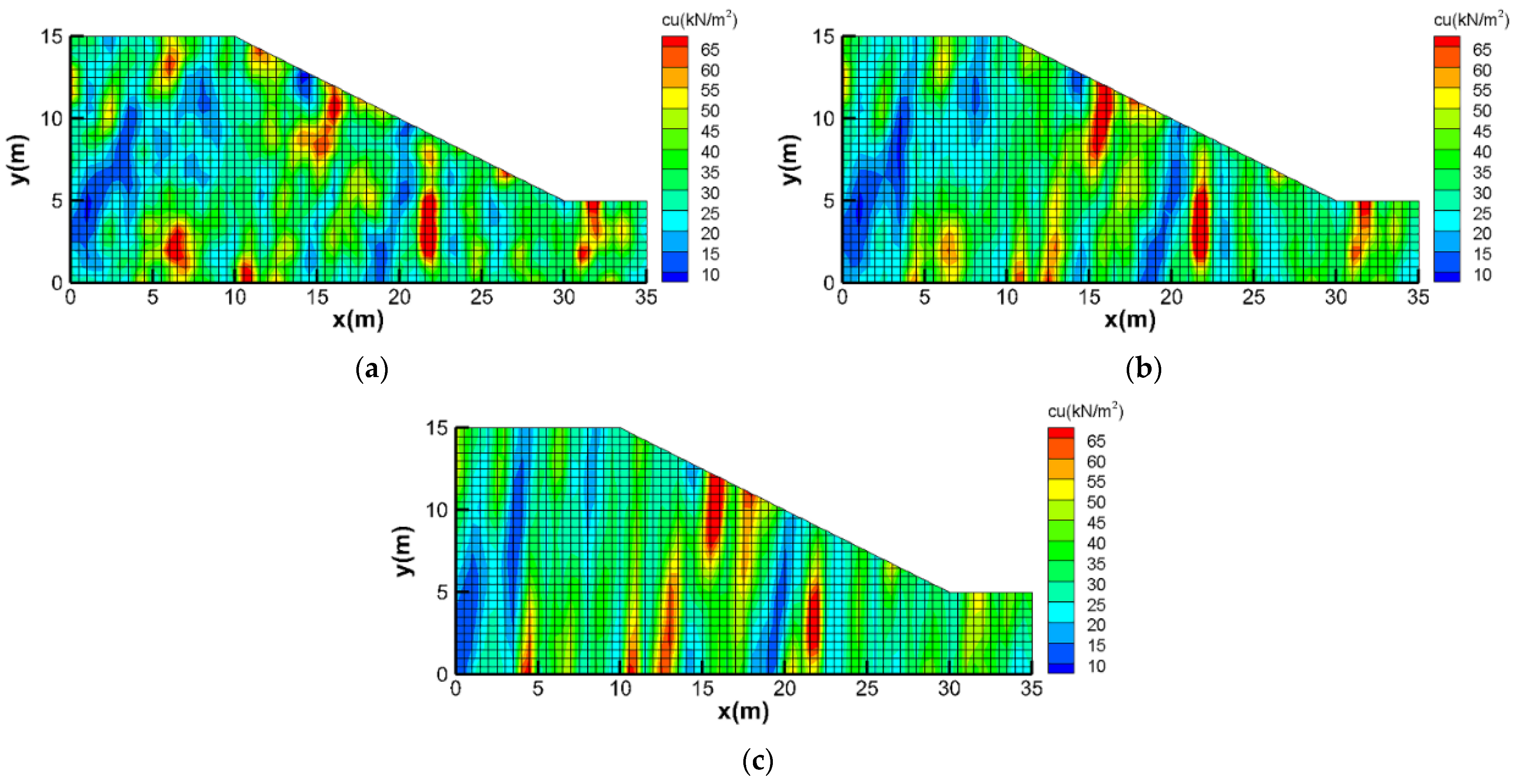
Statistical anisotropic random fields refer to the fact that correlation scales are not equal in each direction (i.e.,
λx is not equal to
λy). Statistical anisotropy is a normal and inevitable feature of heterogeneous geological structures because of the layered distribution caused by large-scale geological sedimentary processes.
Figure 2 displays three different realizations of statistical anisotropic random fields where
λy is equal to 0.5 m and
λx is equal to 2 m, 5 m and 25 m. The random seeds, means and variances of these three realizations are the same as those in
Figure 1. Compared with the statistical isotropic parameter field in
Figure 1, the distribution of their high and low values is the same, but the strong zone and weak zone in
Figure 2 have better horizontal extensiveness. With the increase in
λx, strong and weak zones are increasingly connected in the horizontal direction. Some geological tectonic movements (e.g., folds) may cause the strata to rotate or even stand upright. Therefore, vertical layered slopes are also a common geological phenomenon [
32,
33]. It can correspond to the statistical anisotropy random field in the vertical direction shown in
Figure 3, where
λx is equal to 0.5 m and
λy is equal to 2 m, 5 m and 25 m. The random seeds are different as before, but the means and variances are the same as before. As shown in
Figure 3, similar to the anisotropic random field in the horizontal direction, the strong zone and weak zone are increasingly connected in the vertical direction with increasing
λy.
2.2. Monte Carlo Simulation and Probability of Failure
In this paper, the Monte Carlo simulation (MCS) is adopted to study the effect of the statistical anisotropy of undrained shear strength on
pf. With the given mean, variance and correlation scales, numerous realizations of the spatial distributions of undrained shear strength can be generated using a spectral method [
31].
A synthetic slope model for MCS is created, which is discretized into 1520 square elements with the side equal to 0.5 m (
Figure 1), height H = 10 m and slope inclination
β = 26.6°. The left-side and right-side boundaries are assigned no horizontal displacement conditions and the bottom boundary is assigned no displacement conditions. The soils are assumed to follow the Mohr–Coulomb constitutive models. Additionally, the undrained friction angle
φu = 0 and the unit weight
γ = 20 kN/m
3. The mean of
cu is 34 kN/m
2, according to Griffiths and Fenton [
22] and the standard deviation of
cu is 17. The slope is only subjected to gravity loads. Once these parameters are set up, the corresponding factor of safety for the slope can be evaluated based on the finite element strength reduction method [
34]. For example, the factor of safety of
Figure 1a as the input
cu is 1.05.
Subsequently,
pf can be calculated according to the following formula:
where
Nr is the number of realizations generated during MCS; in this study,
Nr = 500.
NFS<1 is the number of times when the factor of safety is less than 1. When the mean, variance and correlation scales of
cu were obtained, 500 realizations could be generated by using the random field generator mentioned above. For example, when
λx = 0.5 m and
λy = 0.5 m, the
pf evaluated by MCS was 0.470.
3. Results
In this section, the behaviors of the probability of failure (pf) with the change in correlation scales in different directions are investigated. In this paper, λx and λy are 0.5, 1, 2, 5, 10, 25, 50 and 100 m, respectively. That is, the factors of safety of 32,000 realizations need to be evaluated, which requires considerable computing.
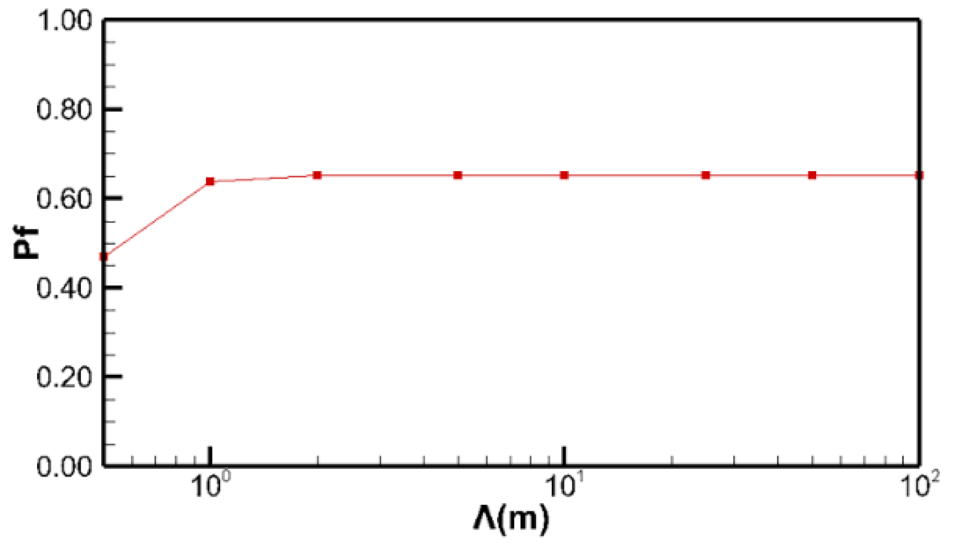
First, the effect of the correlation scale (
Λ =
λx =
λy) on
pf with a statistically isotropic
cu was discussed.
Figure 4 shows the relationship between
pf and correlation scale
Λ. When
Λ is less than 1 m,
pf increases with increasing
Λ (e.g.,
Λ = 0.5 m,
pf = 0.470;
Λ = 1 m,
pf = 0.639). Then, when
Λ > 1 m,
pf gradually stabilizes to 0.651. It can also be concluded from
Figure 1 that when
Λ > 1 m, the influence of correlation scales on the distribution of
cu is gradually reduced so that
pf is eventually constant, which is consistent with the conclusion by Griffiths and Fenton [
22].
Then, the results of
pf with the statistically anisotropic (
λx >
λy)
cu are discussed.
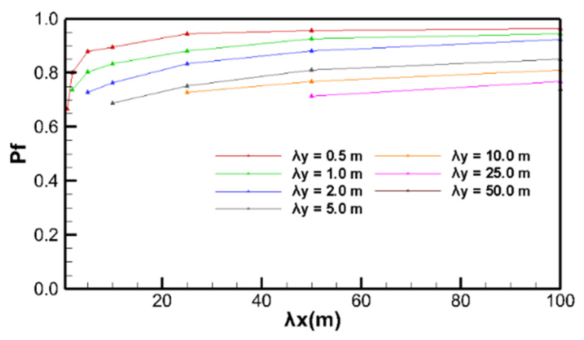
Figure 5 shows the change in
pf with different
λy as
λx increases. It appears that with increasing
λx,
pf has a gradually increasing trend. When
λx is less than the overall length of the slope (the slope length in this study is 20 m),
pf increases rapidly. In the case of
λy = 1 m, when
λx = 0.5 m,
pf = 0.639 and when
λx = 10 m,
pf increases to 0.833, increasing by 0.194. When
λx is larger than the slope length, the increase in
pf becomes less obvious. In the case of
λy = 1 m, when
λx = 25 m,
pf = 0.882 and when
λx = 50 m,
pf only increases by 0.044 to 0.926. Moreover, for different
λy (which means different layer thicknesses), the pattern, i.e., the larger
λx is, the higher
pf is, is the same.
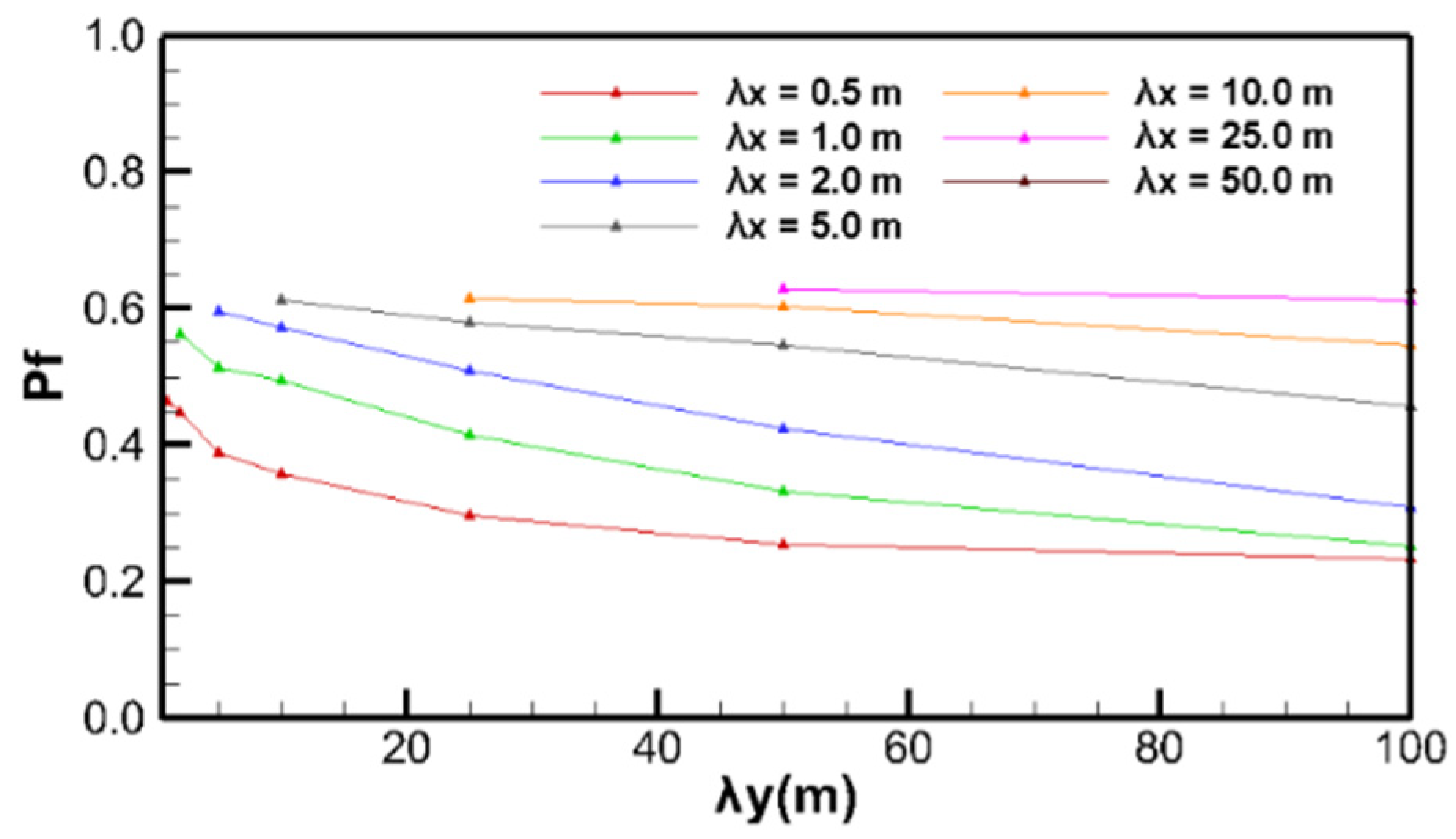
Figure 6 shows the relationship between
pf and
λy with different
λx, where
λy is greater than
λx. Contrary to the pattern of
λx on
pf, with the increase in
λy,
pf decreases under the same
λx. When
λy was less than the slope height (H = 10 m),
pf decreased rapidly and when
λy was greater than the slope height,
pf decreased slowly.
In addition, compared with the condition of statistically isotropic cu, when cu is statistically anisotropic, the variation of λ has a significant effect on the stability of the slope, especially when λx is smaller than the slope length and λy is smaller than the slope height.
According to the above results, it can be easily concluded that in the reliability evaluation of undrained slopes in stratified structures, either the underestimation of λx or the overestimation of λy leads to an unconservative estimate of pf, resulting in an overestimation of the slope stability. This is a more detailed result than previous studies which only considered statistical isotropy and concluded that ignoring the spatial variability of the shear strength parameters could lead to an unconservative estimate of the probability of slope failure.
To ensure that the results of MCS with different correlation scales are representative, the mean of
pf during MCS is examined.
Figure 7 shows that the mean of
pf changes with the increase in the number of realizations for four combinations of correlation scales (
λx = 25 m,
λy = 1 m;
λx = 1 m,
λy =25 m;
λx = 10 m,
λy = 2 m;
λx = 2 m,
λy =10 m). It is accepted that within 200 realizations, the fluctuation of the mean value of
pf is large and after approximately 300 realizations, the mean value of
pf becomes stable.
4. Mechanism Analysis
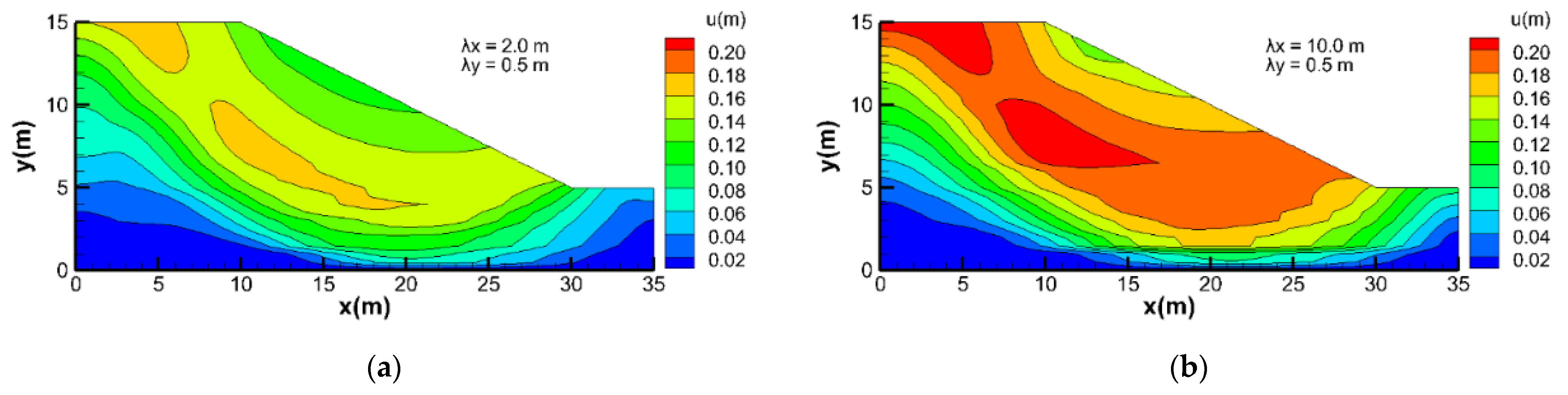
According to the results in the previous section, the longer the horizontal correlation scale is, the higher the probability of failure and the longer the vertical correlation scale is, the lower the probability of failure. The mechanism of this pattern is now investigated based on the displacement distribution of horizontal and vertical layered slopes under gravity.
Figure 8a is the contour map of displacement (
u) corresponding to the parameters in
Figure 2a (
λx = 2 m,
λy = 0.5 m), which has a
FS of 1.03 and the displacement contour in
Figure 8b corresponds to
Figure 2b (
λx = 10 m,
λy = 0.5 m) with a
FS of 0.98. The random seeds of these two realizations are the same; again, the distributions of the strong zone and weak zone are the same, but the degree of connectivity is different. Since the mean and standard deviation of
cu of these two realizations are the same, the magnitude of their displacement is similar in the range. However, under these two sets of correlation scales,
pf calculated by MCS is quite different, when
λx = 2 m and
λy = 0.5 m,
pf is 0.788, when
λx = 10 m and
λy = 0.5 m,
pf is 0.896.
Figure 8 shows that the contour line of the slope displacement distribution is not smooth locally, which is caused by the heterogeneity of the parameter and the slope displacement at the same position is larger when
λx is larger. Comparison of
Figure 8a with
Figure 8b shows that the area where the slope is significantly displaced becomes longer in the horizontal direction since the weak zone is more connected in the horizontal direction. For example, when
λx = 2 m,
λy = 0.5 m, near y = 8 m, the area of maximum displacement extends no more than 5 m in the horizontal direction (
Figure 8a), while when
λx = 10 m,
λy = 0.5 m, at the same elevation, the maximum displacement width exceeds 5 m (
Figure 8b). On the other hand, the yellow area in
Figure 8a extends longer in the sliding direction than the red area in
Figure 8b. It is suggested that a more connected strong zone prevents the development of local displacements as a wall.
However, as the slope is only subject to gravity and the sliding direction is pointing out of the slope, the more connected horizontal weak zone makes the displacement development more unconstrained when λx is greater than λy, resulting in greater slope displacement and, consequently, greater pf.
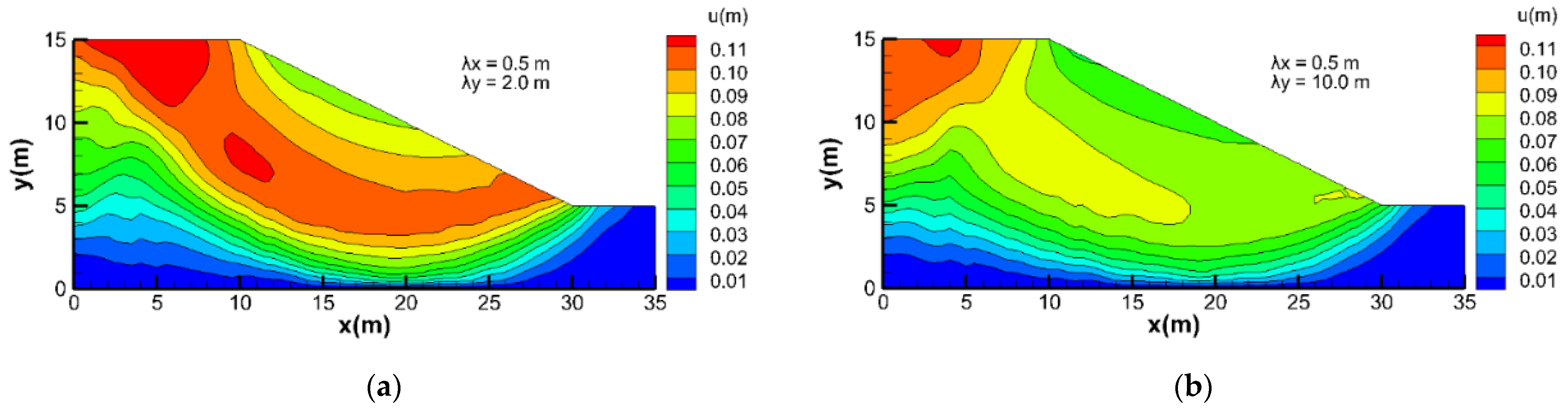
The displacement contour for the case where
λx is less than
λy is shown in
Figure 9, where
Figure 9a corresponds to the parameters in
Figure 3a (
λx = 0.5 m,
λy = 2.0 m), which has a
FS of 1.04 and
Figure 9b corresponds to
Figure 3b (
λx = 0.5 m,
λy = 10.0 m) with a
FS of 1.07.
As can be seen in
Figure 9, the magnitude of displacement is smaller when
λx is smaller than
λy, ranging from 0.01 m to 0.11 m, compared to the case where
λx is greater than
λy. Additionally, the contour line of the slope displacement distribution is also not smooth locally because of spatial variability of the parameter. Moreover, in the case of 9a, a discontinuity of the displacement distribution occurs at X = 9 m and Y = 10 m due to the existence of a strong zone such as an anti-slip pile. Additionally, as
λy becomes larger, the blocking effect of the strong zone becomes more obvious, such that the red area in
Figure 9b is smaller than the red area in
Figure 9a and a new displacement discontinuity appears near X = 6 m, Y = 23 m. Therefore, in the case where
λx is less than
λy, when
λy is greater, the strong zone, such as an anti-slip pile, is more continuous, providing more anti-slip action and increasing the stability of the slope, the displacement decreases and
pf is consequently smaller.
As a summary, an inaccurate assessment of the spatial correlation scales of parameters in slope stability analysis can increase the uncertainty in the calculation of pf and local displacement.
5. Discussion
The accurate description of parameter heterogeneity affects the uncertainty of the slope reliability evaluation. Additionally, the correlation scales reflect the spatial structure of the strata in the slope as an important indicator of the random field theory that quantitatively describes the heterogeneity of the parameters. Due to geological processes, the spatial structure of geotechnical materials is mostly stratified, that is, the correlation scales are not uniform in different directions, also known as statistical anisotropy. However, the effect of correlation scales on the reliability of heterogeneous slopes has rarely been reported in previous studies, which is the reason why this paper investigates the effect of statistical anisotropy of cu on slope reliability.
According to the results of this study, inaccurate statistical anisotropy does lead to significant uncertainty in the slope reliability evaluation, especially underestimating the horizontal correlation scale, which can underestimate the probability of slope failure. Therefore, in practical work on slope reliability evaluation, when the strata are shown to be horizontally stratified through field survey data, the value of cu input to the calculation model needs to be taken very carefully and the use of more complex and detailed geometric models is recommended, especially not to simplify the parameter distribution to homogeneous.
Although this study is limited to synthetic numerical models, it does provide insight into the effect of statistical anisotropy of cu on slope reliability evaluation and demonstrates the importance of the accurate description of the correlation scale for assessment of the probability of failure.
Furthermore, it should be noted that while our discussions focus on the statistical anisotropy of cu, the same stochastic tools can be applied to the analysis of spatial variability of any other parameters and boundary conditions. This refinement is left to future studies. On the other hand, in order to highlight the effect of statistical anisotropy on slope stability, this study conducted a synthetic numerical experiment using unconditional Monte Carlo simulations. If sampling data are available, conditional MCS, which creates realizations that preserve measurements of the primary information at the sampling locations, can be performed to further reduce uncertainty in the slope reliability evaluation and lead to a more accurate probability of failure.
6. Conclusions
This paper introduces the stochastic conceptualization of heterogeneity, which is that the spatial distribution of the parameters can be described with mean, variance and correlation scales. The correlation scales characterize the spatial structure of the strata and when λx is equal to λy, it is called statistical isotropy; otherwise, it is called statistical anisotropy.
Additionally, the effect of statistical anisotropy of undrained shear strength on pf is investigated based on the Monte Carlo simulation. The results show that λx and λy of cu have significant effects on pf. On the one hand, when λx is greater than λy, the larger λx is, the larger pf is, especially when λx is smaller than the slope length, pf increases more significantly. On the other hand, when λy is greater than λx, the larger λy is, the smaller pf is, especially when λy is smaller than the slope height, pf decreases more significantly.
Then, we conduct the displacement analysis of slopes to study the mechanism of the effect of statistical anisotropy on pf. It can be concluded that when λx is greater than λy, the weak zone has a more important influence than the strong zone on slope stability, that is, with λx increasing, the more connected horizontal weak zone makes the displacement development more unconstrained resulting in greater slope displacement and, consequently, greater pf. When λy is greater than λx, the strong zone has a more important influence, that is, with λy increasing, the strong zone, such as an anti-slip pile, is more continuous, providing more anti-slip action and increasing the stability of the slope, the displacement decreases and pf is consequently smaller.
Lastly, it is crucial to accurately estimate correlation scales for the slope stability evaluation, as either the underestimation of λx or the overestimation of λy will result in an underestimation of pf. Therefore, when dealing with horizontally stratified slopes, accurate input parameters and detailed geometric models are recommended.


 and
and 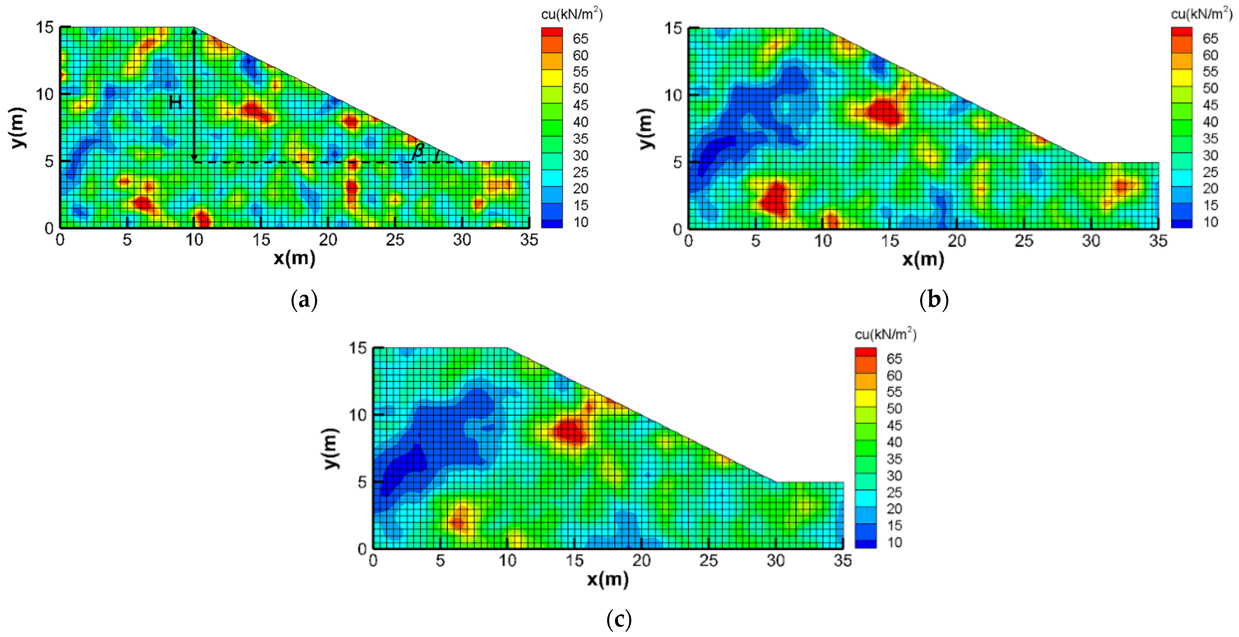


