Abstract
The proposed novel “BathySent” approach for coastal bathymetric mapping, using the Copernicus Sentinel-2 mission, as well as the assessment and specification of the uncertainties of the derived depth results, are the objectives of this research effort. For this reason, Sentinel-2 bathymetry retrieval results for three different pilot sites in Greece (islands of Kos, Kasos, and Crete) were compared with ground-truth data. These data comprised high-resolution swath bathymetry measurements, single-beam echosounder measurements at very shallow waters (1–10 m), and the EMODnet DTM 2018 release. The synthetic tests showed that the “BathySent” approach could restitute bathymetry in the range of 5–14 m depth, showing a standard deviation of 2 m with respect to the sonar-based bathymetry. In addition, a comparison with the “ratio model” multispectral technique was performed. The absolute differences between conventional Earth Observation-based bathymetry retrieval approaches (i.e., linear ratio model) and the suggested innovative solution, using the Sentinel-2 data, were mainly lower than 2 m. According to the outcome evaluation, both models were considered to provide results that are more reliable within the depth zone of 5–25 m. The “ratio model” technique exhibits a saturation at ~25 m depth and demands ground calibration. Though, the “BathySent” method provides bathymetric data at a lower spatial resolution compared to the “ratio model” technique; however, it does not require in situ calibration and can also perform reliably deeper than 25 m.
1. Introduction
Nowadays, the determination of nearshore bathymetry is essential for multiple applications, i.e., research activities, such as the investigation of submarine morphodynamics, coastal erosion, tsunami propagation toward the coast, and climate change initiatives, as well as operational activities by local authorities and decision makers. Such knowledge is crucial for planning sustainable coastal development, coastal risk assessment (including the tsunami hazard), and sustainability of submarine ecosystems. Moreover, coastal bathymetry represents a critical contribution to the nearshore navigation and investigation of submarine resources.
The proposed, by the current study, BathySent solution is an application of a novel algorithm to Sentinel-2 data to decisively deal with a variety of essential issues referred to below:
- (i)
- Optimization of dredging operations (e.g., identification of the migration of sandbanks hindering navigation). The coastal zone is a dynamic environment and modern echosounders have not yet been designed to perform routine monitoring of shallow bathymetry, while the survey vessels equipped with bathymetric sonar systems very often cannot approach shallow-water areas (even up to 30 m) due to reef occurrence or hummocky seafloor.
- (ii)
- Natural hazard assessment. Naturally occurring physical phenomena, e.g., storm waves, tsunamis, and mass wasting events, are a great threat to several very shallow, densely populated coastal areas whose monitoring is of key importance for the understanding of the hazards and their principal causal agents (i.e., climatic, meteorological, and geophysical). This can be only accomplished by remote sensing techniques.
- (iii)
- Surveillance of aquaculture, fisheries, and benthic habitats. Shallow bathymetry maps produced by the repeated satellite passes over areas not accessible to humans may reveal evolving ecosystems.
- (iv)
- Assessment of the condition of accessibility/disembarkation in remote coastal zones for military/humanitarian operations.
- (v)
- Major contribution to the planning of a successful archaeological survey in very shallow submerged prehistoric landscapes.
2. Review of Imagery Analysis Techniques for Coastal Bathymetry Estimation
For the performance of a remote survey to determine nearshore bathymetry, several remote sensing techniques have recently been applied either to retrieve water depths directly, or even indirectly, using depth inversion modeling via estimation of water surface movements. The direct measurement methods are based on the fact that the light penetrates into different depth levels at various wavelengths in the water column, while the methods that estimate bathymetry indirectly are based on measuring water surface characteristics. The latter approach models the nearshore bathymetry inversely by estimating depth-induced wave properties from remotely captured images, identifying waves, and using wave dispersion relationships.
2.1. The Multispectral Approach (Direct Method)
The technique uses the radiance of passive multispectral imagery, based on the extinction of light with water depth [1,2,3,4]. Even though the method provides coastal bathymetry with a high spatial resolution (equal to the resolution of the imagery), the derived results depend on the water quality, seabed reflection, and atmospheric effects. The achieved precision is ~20% within the 0–6 m depth range [4]. Since the technique requires in situ values for calibration, it is not applicable in non-accessible areas or turbid waters. The good performance of the approach highly depends on the seawater clarity and usually requires empirical algorithms for the retrieval of water depths, due to optical complexities caused by scattering and attenuation of the incident light in the water column, and bottom reflection as well. For the direct extraction of coastal bathymetry, spectral satellite/airborne technology [5,6,7,8,9,10,11] and light detection and ranging (LiDAR) technology [12] have been suggested.
Benny and Dawson [6] and Bierwirth et al. [7] demonstrated retrieval of water depths using a Landsat multispectral scanner and a Landsat thematic mapper sensor, respectively. Benny and Dawson [6] detected and contoured shallow-water areas and shoals with depths less than 18 m in the northern Red Sea, while Bierwirth et al. [7] surveyed Shark Bay in Western Australia, with their method, however, overestimating the water depths by several meters. Sandidge and Holyer [9] processed hyperspectral data, obtained from an airborne visible/infrared imaging spectrometer (AVIRIS), to estimate the nearshore bathymetry in Tampa Bay in Florida as well as in other Florida sites having depths ranging from 0 to 6 m. When the retrieved depths were compared to ground truth data, the calculation of the Root Mean Squared Error (RMSE) provided values of 0.84 m and 0.39 m, respectively. In Tampa Bay, an AVIRIS technique was also applied by Lee et al. [8] to survey water subsurface properties based on a model-driven optimization algorithm without prior knowledge of the water’s optical properties. The retrieved depths ranged from 0.3 to 4.6 m. Further, Adler-Golden et al. [5] applied a physics-based algorithm, which uses minimal ground truth inputs to AVIRIS data, littoral airborne sensor hyperspectral data, and multispectral (QuickBird) imagery, to estimate the seafloor topography in Kaneohe Bay in Hawaii, and in Tampa Bay as well. The precision of the retrieved depth values was within 2–3 m over a 0–10 m depth range. Finally, the LiDAR-based method of Irish and Lillycrop [12], named SHOALS, achieved the retrieval of much deeper depths compared to the previous multispectral techniques, estimating water depths up to 60 m with a precision of ~15 cm.
2.2. Depth Inversion Approach: The Wave Dispersion Relationship (Indirect Method)
The methodology is based on Fast Fourier Transform (FFT) and timestack techniques, computing water depths by relating wave parameters, such as wave period (T) and wavelength (L), and current velocity (U), with the general form of the Airy surface gravity wave dispersion formula:
where ω (defined as 2π/T) is the angular frequency, g is the gravitational acceleration, h is the local water depth, Uvector is the vector of the mean water velocity, and kvector (kx and ky) is the vector of the wave number k (defined as 2π/L). Since water waves become less dispersive and wave phase speed (or wave celerity) is more strongly dependent on depth rather than on the wave parameters as waves propagate toward shallower waters, the wave phase speed (c) has been more practically used for depth determinations by substituting the angular frequency and wave number in the following equation:
with the assumption that U and k are zero. In deep waters (kh > 0.5), Equation (2) simplifies to:
where Lo is the deep-water wavelength obtained from Equation (1), with no currents and the deep-water assumption as:
while based on Equations (2) and (3), the celerity of a wave propagating from deep water toward shallower water can be expressed as:
ω = [gk tanh(kh)]0.5 + Uvector kvector,
c = ω/k = (g/k) tanh(kh),
co = (g/k)0.5 = g/ω = gT/2π = Lo/T,
Lo = gT2/2π,
c = co [tanh(kh)]0.5,
In shallow water and/or long wavelengths (kh < 0.05), the approximation of Equation (2) becomes:
which is a function of water depth only, being independent of the wave number k. However, a number of previous studies have shown that the shallow water linear dispersion relationship underestimates the wave speed within the surf zone, close to the shoreline, because of the finite amplitude effects.
c = (gh)0.5,
There are several different ways to classify the depth inversion methodology:
- Frequency domain inversions or time domain inversions;
- Theoretical or full approaches;
- Inversions based on depth-induced spatial water surface variation;
- Inversions based on depth-induced wave property or based on wave-breaking generated dissipation patterns;
- Inversions based on field or synthetic data.
A variety of depth inversion methods have been developed along with advances in various remote sensing techniques. Each of the remote sensing platforms has its own limitations as well as advantages over others in terms of image resolution, spatial image coverage, and temporal image collection. For this reason, several different approaches for remotely estimating littoral seafloor topography can be considered depending on the input image data types.
The airborne optical platforms allow much more orthogonal measurements over the sea surface than shore-mounted platforms as well as continuous sampling wave imagery at high frequencies over a target area at a time scale ranging from an hour to a day, flying around the area of interest.
In contrast to locally operated platforms, a satellite orbit around the Earth acquires only one snapshot image or sample wave images over a target area for a few seconds. For cases where the surface information is collected sparsely in time, Dalrymple et al. [13] developed two depth inversion methods applying the Hilbert transform and lag-correlation techniques to two sequential images. In fact, Dalrymple et al. [13] numerically generated two sequential surface elevation maps with a reasonably short time interval, instead of using actual images.
Currently, operating satellites acquire images in a sparse time-lapsed fashion, except for SkySat, which records videos of the Earth’s surface, but its data are not freely available to the public.
2.3. Satellite Methodology Based on the Wavelength and Surface Wave Parameters
This depth inversion approach is based on the analysis of wave propagation and does not require temporally dense image sequences, utilizing one or two sequential images of wave phase or surface elevation maps over a reasonably short time interval less than the wave period. Leu et al. [14] and Leu and Chang [15] used the previous methodology for the retrieval of water depths lower than 12 m from two SPOT satellite images taken in deep and shallow water regions. Assuming that waves are propagating from deep to shallow waters, initially, the dominant deep-water wavenumber and wave frequency are estimated from 2D wave phase information of the deep-water image. Then, the 2D wavenumber spectrum of the shallow water image is analyzed to derive the water depth based on the linear dispersion relation. The physical distance of the sampling window is 200 m (32 pixels), which, however, is not adequate for the nearshore section close to the coastline. In addition, the effect of the nonlinear wave amplitude dispersion contributes significantly to the errors of the depth inversion approach in the nearshore area via the linear dispersion relationship.
When the water depth is less than half the dominant wavelength, the latter decreases toward the coast due to the water depth reduction. It is then possible to estimate the water depth knowing the dominant wavelength and the wave period by using the linear wave theory. This method has been applied since at least the World War II (Wilson, 1942). However, the spatial resolution is often reduced by the calculation of the wavelength. The application of the method to satellite images, in the optical domain, has rarely been reported in the scientific literature [14,16]. In the study of Leu et al. [14], an average error of 17.5% in relation to the ground truth bathymetry was calculated for the 0–15 m depth range at a spatial resolution of 400 m. It should be emphasized that for the good performance of this method, the determination of the wave period is crucial, which may be obtained from ancillary data or through a priori knowledge of some water depths.
Recently, Danilo and Melgani [17] developed a technique based on Landsat-8 images to extract bathymetry. They propose a method based on combining wave tracing and linear wave theory for the estimation of wave period and bathymetry in coastal areas. Even though the method was developed for Landsat imagery, it can be applied to different types of satellite optical images. The experimental results of the aforementioned study were obtained from several sites located around the Hawaiian Oahu Island and were derived from the analysis of 13 Landsat-8 images. The output showed that the wave period estimates were compatible with the wave buoy measurements in all cases. In addition, the retrieved bathymetry data displayed a Standard Deviation of less than 15% of the actual depth out of the surf zone down to 20 m, for sites characterized by a direct exposure to swell and an absence of clouds. The suggested method does not rely on ancillary data and works using satellite images in which waves are present.
3. The BathySent Algorithm
3.1. Innovative Aspects
The “BathySent” solution presented in this study is actually a ‘clever’ modification of the Poupardin et al. [18] correlation, wavelets, and bathymetry (CWB) method, with the central concept being the production of pairs of wave celerity and wavelength from Sentinel-2 data, which can efficiently retrieve water depth values through the linear wave dispersion relationship:
where is the water depth, is the swell wavelength, is swell celerity, and is the standard acceleration due to gravity equal to 9.81 m/s2. The BathySent algorithm details are presented in de Michele et al. [19]. In some way, the CWB method, in its initial form, can be seen as a demonstrator (already applied to SPOT-5 data) of bathymetry retrieval from wave characteristics obtained through inter-band image correlation, but not as an operational method. Theoretically, if the current form of CWB applies to any push-broom sensor, the resulting algorithm will be excessively slow for processing data concerning extensive coastal areas. The reasons rest in the fact that CWB is based on repeated wavelet decomposition for the estimation of the dominant wavelengths and orientation, while it applies spatial correlation to the computed wavelets in order to associate celerity with the identified dominant waves. On the other hand, the CWB procedure does not take advantage of the simultaneous computation of wavelength and wave celerity in the spatial frequency domain. Therefore, modifications to the BathySent algorithm CWB method can establish a technique, which will process much faster Sentinel-2 images of extensive coastal areas (the swath in the Sentinel-2 images is ~250 km). Hence, in order to accomplish the CWB modification, FFT-based methods were used to produce the spectrum of the local waves together with their associated celerity, while the combination of the local Fourier spectra of different Sentinel-2 bands, which included both spatial frequency and phase, derived the significant celerity/wavelength pairs. Moreover, for the operational implementation of the modified CWB method into a platform, two more activities need to take place:
- Adaptation of the produced algorithm as a Python code for its convenient implementation;
- Identification of additional functionalities required for easy use; i.e., the capability of selecting co-registered images featured by decreased cloud cover and clearly visible wave fields with diverse wavelengths and directions.
Further, for the adaptation of the modified CWB method (which was designed for SPOT-5 data) to the Sentinel-2 data, the main characteristics of the sensors associated with both optical Earth-imaging satellites had to be considered:
- The resolution of Sentinel-2 imagery is 10 m, while that of SPOT-5 is 2.5 and 10 m for panchromatic and multispectral images, respectively. Hence, the Sentinel-2 data resolution is a limitation for the precision of image correlation, which is expected to be between 1/2 and 1/10 pixels. In addition, the theoretically detected wavelength is restricted by Shannon’s threshold to twice the pixel size;
- The longer (5-day) repeat cycle of Sentinel-2 is of major interest because it enhances image precision by cumulating wave states of different dates (i.e., using waves with different directions and wavelengths) and allows the acquisition of a larger archive that can provide images with reduced cloud cover and good visibility of significant waves;
- The time span between the sensors’ bands is 0.6 s for Sentinel-2 (between B2 and B4) and 2 s for SPOT-5 (between the panchromatic and multispectral images).
Hence, the resulting celerity estimation from Sentinel-2 data is going to be less precise. However, the spectrum combination method suggested by the BathySent solution offers the possibility of using three bands (e.g., Red, Blue, and Near-Infrared) or even more for the enhancement of precision. For the recording of an image line, the Sentinel-2 sensor uses a set of 14 charge-coupled device (CCD) modules instead of a single CCD module used by the SPOT-5 sensor. For technical reasons, two adjacent modules in the Sentinel-2 sensor are inverted, i.e., if the first module records B2 before B4, the second module will record B4 before B2. This results in a time inversion if we consider B2 as a reference. Even though the sign of wave celerity does not have any impact on the wave dispersion relation (which uses the absolute value of the displacement), the correlation at the border between the two neighboring modules can fail, resulting in narrow bands (about half of the correlation window), where information is lost. However, the data gaps can easily be filled by interpolation.
3.2. The Joint Use of Wave Celerity and Wavelength
The method relies on the linear wave theory and uses two consecutive images with a time delay of a few seconds to measure wave celerity [18,20,21,22,23,24]. In addition, more than one swell wavelength contributes to the bathymetry estimation and this allows for the increase in the final resolution compared with other solutions. Using this method, Mancini et al. [21] retrieved depths exhibiting deviations of 20% from the actual water depth (ranging from 4 to 16 m) for a spatial resolution of 125 m. The method can also be used for the estimation of sea surface currents, but its main drawback is the limited number of images available with the required short time delay.
With the wave celerity measurement in addition to the wavelength estimation, the problem of wave period is instantly resolved. Abileah [20] using IKONOS stereo pairs introduced the measurement of wave celerity from optical satellite data. De Michele et al. [22] improved the method by using the small time lag between two bands of a SPOT-5 dataset, while Danilo and Binet [23] have detailed the concept and limiting factors. Likewise, with other methods, this technique takes advantage of the wave dispersion relationship expressed by Equation (3). However, it is more robust, in principle, because it is based on the joint use of independent measurements of wave celerity and wavelength. This technique is actually analogous to the BathySent algorithm and, to the best of our knowledge, has been successfully applied to satellite datasets by Abileah [20,25], Mancini [21], and our team [18,19,22,24]. Bergsma et al. [26] proposed a method based on multiple Sentinel 2 bands and the Fourier slice theorem. Almar et al. [27] proposed a method to extract bathymetry from the Pleiades satellite’s “persistent” mode, based on (c, L) measures.
The study of de Michele et al. [22] showed that wave celerity may be measured by a cross-correlation algorithm based on the time lag between quasi-simultaneous acquisitions of two spectral bands from a single passage of a satellite platform. Even though the relevant algorithm was applied to SPOT-5 imagery, it can virtually be applied to all the push-broom sensors that show CCD offsets on the instrument’s focal plane. On this basis, Poupardin et al. [18,24] suggested a local spectral decomposition prior to the wave celerity estimates in order to produce local celerity and wavelength pairs for the water depth determination, using the dispersion relationship. During the performance of the methodology, for every wavelength, the backward wavelet transform is calculated in order for the estimation of wave celerity to be performed by local correlation in the real domain. This procedure has the disadvantage of the computing cost. Hence, in the BathySent concept, we make a step forward by calculating the wave celerity as the phase shift of the Fourier transforms between a number of Sentinel-2 bands, thus reducing the computing cost.
The BathySent concept originates from the method developed in the study of de Michele et al. [22] and Poupardin et al. [18]. The BathySent concept also relies on the fact that Sentinel-2 is capable of the correct imaging of the swell, which allows a valid computation of the swell spectrum, as recently presented in Kudryavtsev et al. [28,29]. The BathySent algorithm uses multiple bands from Sentinel-2, each of which is acquired with a characteristic time delay ranging from 0.5 to 2 s. The bands are resampled to the highest resolution available (10 m) and the Fourier spectrum is calculated. The algorithm scans the spectrum and searches for instantaneous frequencies related to the most energetic wavelengths. The phase differences for each selected frequency are calculated among all Sentinel-2 bands and are converted to swell phase velocities, yielding a set of wave celerity and wavelength couples. These couples are, then, used in the wave dispersion relationship to retrieve the water depth. The Sentinel-2 dataset is scanned on the base of a moving window, yielding water depths at each step of the grid creation. This grid defines the final spatial resolution of the bathymetric map. The resolution of the estimated depths is imposed by the physics of the phenomenon (i.e., the wave dispersion relationship) and typically ranges from L/2 to L/20. Therefore, in the Mediterranean Sea, where swells have wavelengths usually less than 40–60 m, the BathySent algorithm is anticipated to retrieve depths up to 20–30 m. However, the estimated depths in ocean basins should be higher because the swell could potentially reach larger wavelengths.
3.3. Prerequisites for the Combined Application of Wave Celerity and Wavelength
For the good performance proposed by this study’s solution, the swell needs to be clearly imaged by the sensor and the following criteria should be fulfilled:
- Absence of clouds.
- Occurrence of turbid water. If the seawater is transparent the swell might not be clearly visible in the satellite dataset.
- Favourable geometry between the sun, sensor, and wave fronts (see [23]) as well as imagery of swells with diverse periods or wavelengths.
- Optimum image resolution as well as the existence of two pixels at least for the measurement of the smallest wavelengths.
- Satellite dataset including more than 20 acquisitions.
In addition, it should be noted that the resolution of the final bathymetric grid will be lower than the one retrieved by the multispectral method (due to the window size of the 2D correlation), while the cost of the data acquisition could be a limiting factor if a certain amount of them has to be used for the improvement of the precision of the final output.
3.4. Sentinel-2 Data Suitability for the BathySent Algorithm
The first advantage of the Sentinel-2 data is the frequent acquisition of images, which statistically enhances the potential of the obtained datasets to fulfill all criteria mentioned above, while the acquired data become available free of charge.
The second advantage is that the focal plane geometry of Sentinel-2 is undisclosed. Therefore, we know exactly what are the time lags between multiple bands.
The third advantage is that the Sentinel-2 datasets offer the possibility for multiple bands (with multiple time lags) to be jointly used within a single run on our processor. This yields different measurements of wave celerity and wavelength, which are vital for the improvement of the precision of the final output.
Finally, even though the pixel size (10 m) of Sentinel-2 images is a limiting factor for very shallow bathymetry retrievals (0–10 m), the ability of our correlator to measure sub-pixel offsets could partially fill this gap. On the other hand, data obtained from third-party missions, affording very high-resolution sensors, might be complementarily used.
4. Materials and Methods: Study Area and Reference Bathymetric Data
In order to test the performance of the BathySent algorithm, three pilot sites in the south Aegean Sea (Kos and Kasos islands and Cretan Sea—Chania Gulf—Crete Island) (Figure 1) were chosen, and the uncertainty level of the retrieved bathymetric data was determined through comparison to reference datasets. The uncertainty assessment was carried out using the RMSE and mean absolute error (MAE) as well as the statistical Bland–Altman plots [30,31,32]. The latter graphical analysis allows the identification of any systematic difference between two measurement methods (i.e., fixed bias) or potential outliers, with the mean difference being the estimated bias and the Standard Deviation of the differences, revealing the fluctuation around this mean. Moreover, a conventional Earth observation (EO)-based bathymetry retrieval approach, i.e., the linear ratio model of Stumpf et al. [6], was applied to the Level-1C Sentinel-2 imagery (mission of 2019) of one of the pilot sites (i.e., Kos Island; Figure 1) in order to retrieve a bathymetric dataset to be statistically compared with the corresponding BathySent solution output.
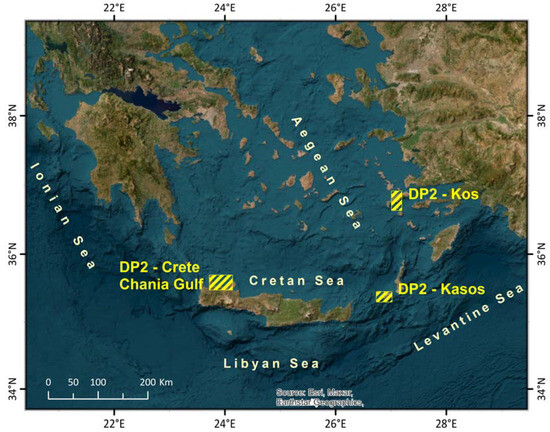
Figure 1.
Location of the pilot sites in the south Aegean and Cretan seas (Greece).
Three bathymetric data packages, i.e., DP1, DP2, and DP3, associated with the three selected Greek pilot sites (Figure 1), respectively, were derived from the application of the BathySent algorithm to Sentinel-2 data (mission of 2018 for DP1, DP2, and DP3 plus mission of 2019 for DP2 and DP3) and, subsequently, evaluated using the following reference datasets:
- The EMODnet digital terrain model (DTM) of 2018 (for DP1 and DP2) at a resolution of 1/16 arc minute (~120 m), downloaded from the EMODnet portal (https://portal.emodnet-bathymetry.eu/, accessed on 14 September 2018).
- Survey data from the repository of the Hellenic Centre for Marine Research (HCMR) (for DP2);
- Data from recent bathymetric surveys (for DP3) carried out by HCMR.
In more detail, the data sources of the reference DTM related to DP1 were the General Bathymetric Chart of the Oceans (GEBCO) 30 arc-second global grid, resampled to 3.75 arc seconds (published in 2014 and updated in 2015), as well as satellite-derived bathymetry (https://sextant.ifremer.fr/record/SDN_CPRD_4667_greece1007/, accessed on 20 July 2023). However, it should be noted that it was not feasible to evaluate the uncertainty level of the satellite-derived bathymetry due to the lack of modern survey data acquired via acoustic or LiDAR technology.
The reference bathymetry for the northwestern coastal area of Crete was also downloaded from the EMODnet portal (DTM of 2018) and was based on the following sources:
- Datasets from multibeam and single-beam surveys were carried out by HCMR in 2015, while their metadata are available from https://cdi-bathymetry.seadatanet.org/report/edmo/269/gn36201500007_269_g74 (accessed on 20 July 2023) and https://cdi-bathymetry.seadatanet.org/report/edmo/269/gn36201409922_269_g74 (accessed on 20 July 2023), respectively.
- Satellite-derived bathymetry provided by EOMAP (https://sextant.ifremer.fr/record/SDN_CPRD_4667_greece1001/, accessed on 20 July 2023).
- GEBCO 30 arc-second global grid, upsampled to 3.75 arc seconds
Almost the entire study area is covered by in situ data acquired by HCMR using single and multibeam ecosounders in 2015 and integrated into EMODnet DTM in 2018. The authors preferred to use the EMODnet DTM rather than the raw data directly since the data had been integrated into the EMODnet and it was allowed by the spatial resolution of the analysis (i.e., 80 m).
For the validity assessment of the bathymetric output for Kos (DP3), multibeam and single-beam recordings (recently acquired) were used as reference datasets. The swath bathymetry data were obtained onboard R/V Alcyone (HCMR) during a 4-day cruise carried out in 2019 (8–12 October). A seabed area of 25 km2, with the water depths ranging from 4 to 40 m, was surveyed at an average navigation speed of 4 Knots, using a hull-mounted Teledyne RESON SeaBat 7125 dual-frequency (200/400 kHz) echosounder. During the cruise, the accuracy of the bathymetric data positioning was enhanced by a Coda Octopus F185+R GPS RTK system, achieving uncertainties within a few centimeters. The collected data were post-processed by the Teledyne RESON PDS2000 software, including the removal of spurious soundings, noise filtering, and tide and sound velocity profile corrections. A DTM was produced by Esri’s GIS mapping software (ArcGIS Desktop 10.5–10.8), having a resolution of 2 m. In addition, the single-beam bathymetry data were collected at very shallow waters (2–10 m), using a Humminbird Helix 9 Chirp Mega SI GPS G2N sonar. The sonar transducer was mounted on the side of an inflatable boat, which navigated at an average speed of 5 knots. The 200 kHz operating frequency was selected in order to take full advantage of the sonar’s optimum resolution. Depths were recorded at steps of 1 pulse s-1 along tracklines of a total length of 50 nmi, while the echosounder’s GPS/WAAS receiver provided a horizontal uncertainty within 2.5 m.
5. Results—Assessment of the BathySent Algorithm Performance over the Pilot Sites in the Aegean Sea
5.1. Kasos Island Bathymetric Data Package (DP1)
The BathySent-derived bathymetry of Kasos Island (obtained from the Sentinel-2 mission of 2018) in ENVI format (Figure 2a) was georeferenced in a UTM 35N coordinate system (EPSG 32635) with positive values toward deeper bathymetry and a spatial resolution of 160 m resolution. Then, the image was processed and converted into an ESRI raster geodatabase format in order for all the analyses to take place via the ArcGIS suite. The BathySent result image was then studied/analyzed regarding the depth values. The retrieved depths were up to 20 m, with the covered area extending much deeper (Figure 2b).

Figure 2.
(a) The initial ENVI format of the depths derived from the BathySent solution applied to Sentinel-2 data (mission of 2018) for Kasos Island (south Aegean Sea); (b) The output from the application of the BathySent algorithm to the 0–20 m depth zone (160 m resolution).
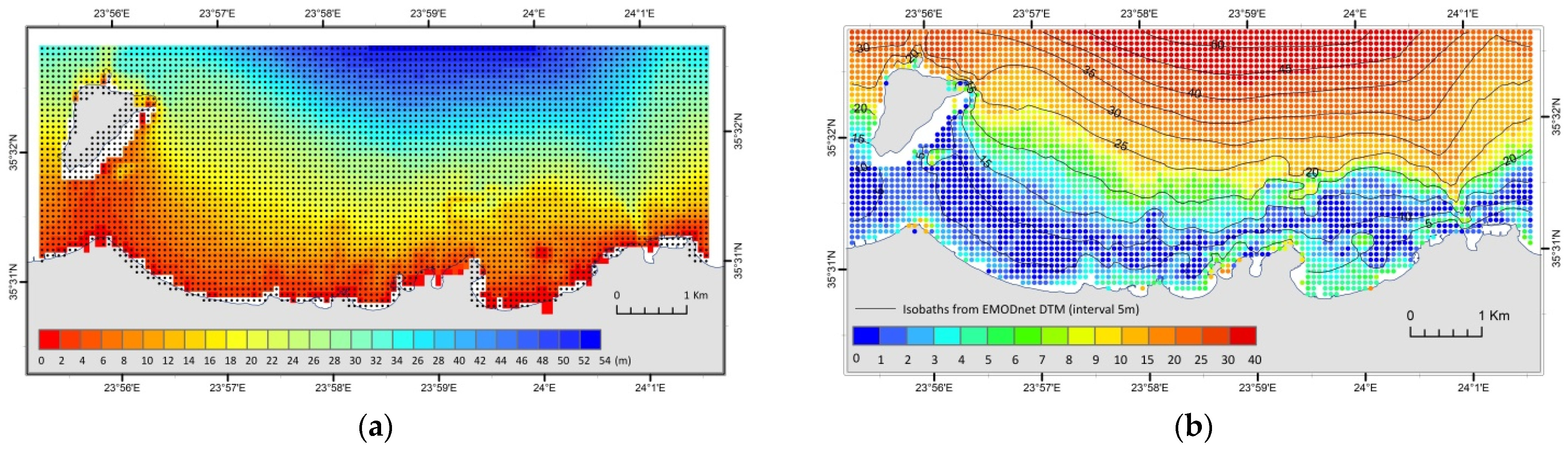
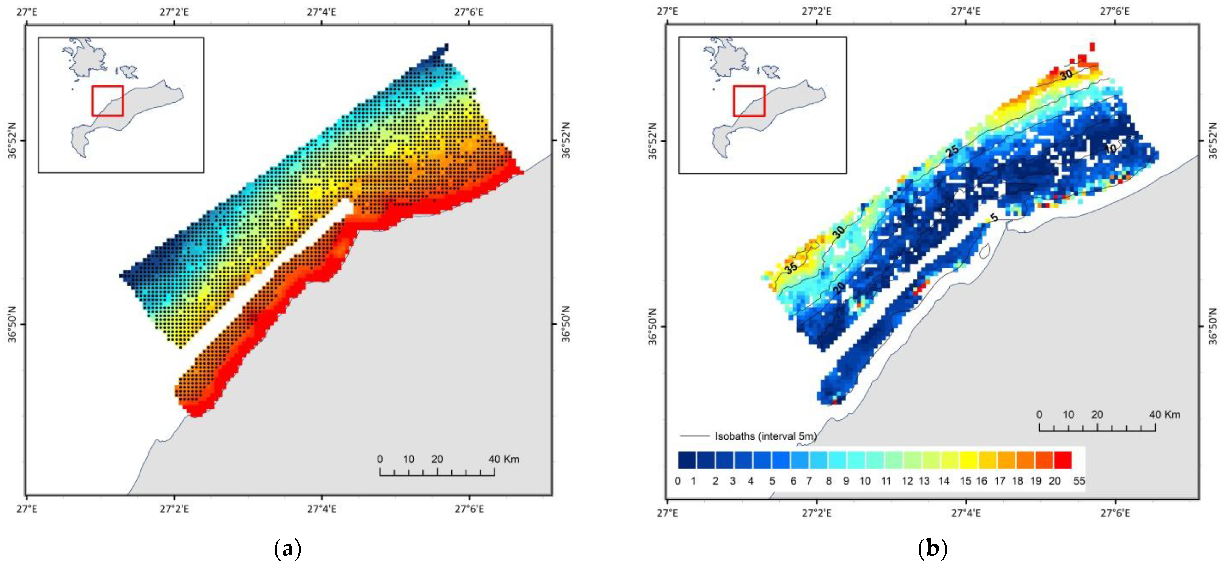
The validity of the bathymetric output was assessed by its comparison with a DTM of the 0–60 m depth interval (Figure 3a) obtained from the EMODnet High-Resolution Seabed Mapping Lot. The reference DTM was resampled to match the spatial resolution and extent of the bathymetric raster image derived from the Sentinel-2 data and the BathySent algorithm. The latter image was converted into a vector-point dataset (Figure 3b), which was compared to the corresponding dataset of the EMODnet bathymetric grid. Hence, the differences between the values of the Sentinel-2 bathymetric DTM and the EMODnet DTM were calculated (Figure 3c), providing the basis for the subsequent statistical assessment.
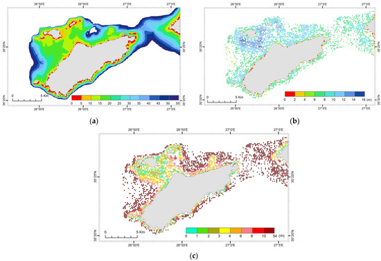
Figure 3.
(a) EMODnet bathymetry (0–60 m depth zone) for Kasos Island (resolution of ~120 m); (b) vector-point feature of the BathySent algorithm results for the 0–17 m depth zone; (c) Absolute differences (m) between the two measures. The displayed 5 m interval isobaths were derived from the EMODnet DTM.
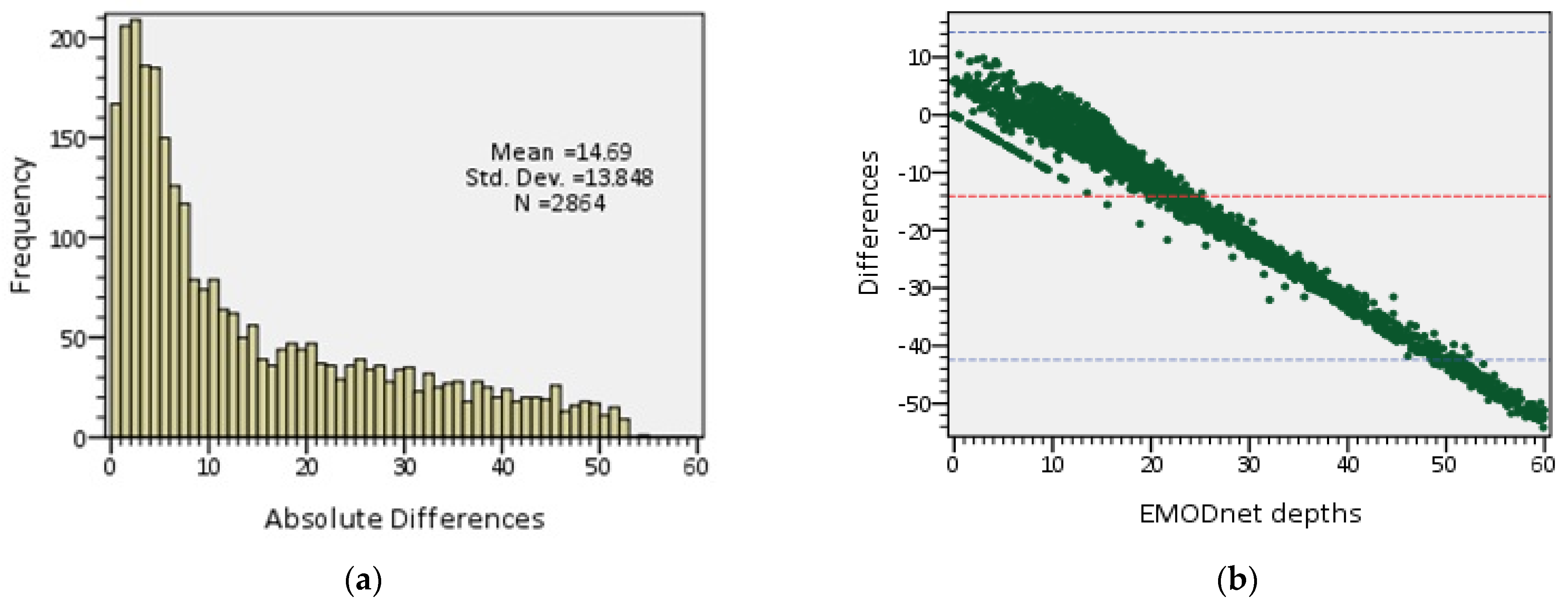
Figure 4 and Figure 5 illustrate the histograms of the frequencies of the absolute differences between the Sentinel-2-derived depths and the reference EMODnet bathymetry as well as the Bland–Altman statistical plots for the 0–60 m and 0–17 m depth intervals, respectively. The analysis revealed that in the shallower depth zone, the BathySent algorithm performed better, providing MAE and RMSE values of 3.82 m and 4.56 m, respectively. In contrast, for the deeper depth interval, the MAE and RMSE appeared considerably higher (14.69 m and 20.19 m, respectively). In particular, for the 0–17 m depth interval (Figure 5a), 25% of the observations were lower than 1.8 m, 50% did not exceed 3.5 m, and 75% reached up to 5.4 m, suggesting a reasonably good agreement of the BathySent algorithm results with the reference bathymetry. The previous interpretation was further supported by the Bland–Altman plot, showing an acceptable 95% confidence interval width and a low mean difference (i.e., 2.5 m) (Figure 5b), indicating an interchangeable use of the two datasets.
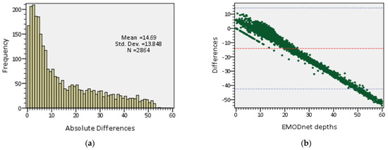
Figure 4.
Depth zone of 0–60 m: (a) Frequency histogram (counts)of the depth differences (m) between the Sentinel-2 bathymetric data and the EMODnet reference bathymetry (m); (b): Bland–Altman statistical plot assessing the degree of agreement between the two measures, the 95% confidence limits are shown (mean ± (1.96 × st.dev) red and blue lines).
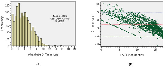
Figure 5.
Depth zone of 0–17 m: (a) Frequency histogram (counts) of the depth differences (in m) between the Sentinel-2 bathymetric data and the EMODnet reference bathymetry (m); (b) Bland–Altman statistical plot assessing the degree of agreement between the two measures, the 95% confidence limits are shown (mean ± (1.96 × st.dev) red and blue lines).
5.2. Crete Island Bathymetric Data Package (DP2)
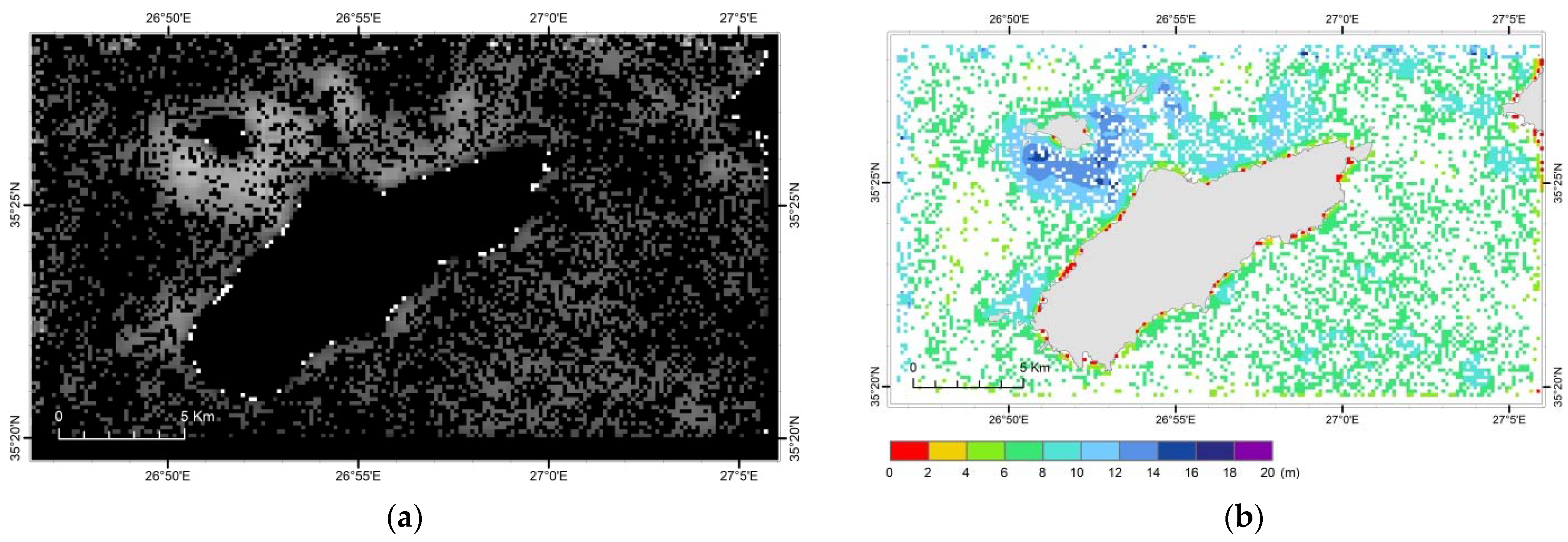
The initial data (from the northwestern coastal part of Crete) were obtained from the Sentinel-2 missions of 2018 and 2019; not all the data were suitable for the BathySent solution but three acquisitions were, finally, found where the algorithm could perform the best. Likewise, with DP1, the retrieved bathymetry was provided in ENVI format georeferenced to the UTM 34N coordinate system, in double precision coding, with positive values toward deeper bathymetry and having a spatial resolution of 80 m (Figure 6a), which was, then, transformed in an ESRI raster geodatabase format (Figure 6b).
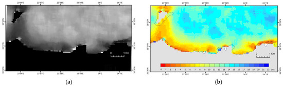
Figure 6.
(a)The initial ENVI format of the depths derived from the BathySent solution applied to Sentinel-2 data (missions of 2018 and 2019) for the northwestern coastal area of Crete Island (Cretan Sea); (b) Sentinel-2 bathymetric raster image of the 0–30 m depth zone (80 m resolution).
For the assessment of the bathymetric output, the steps described below were followed:
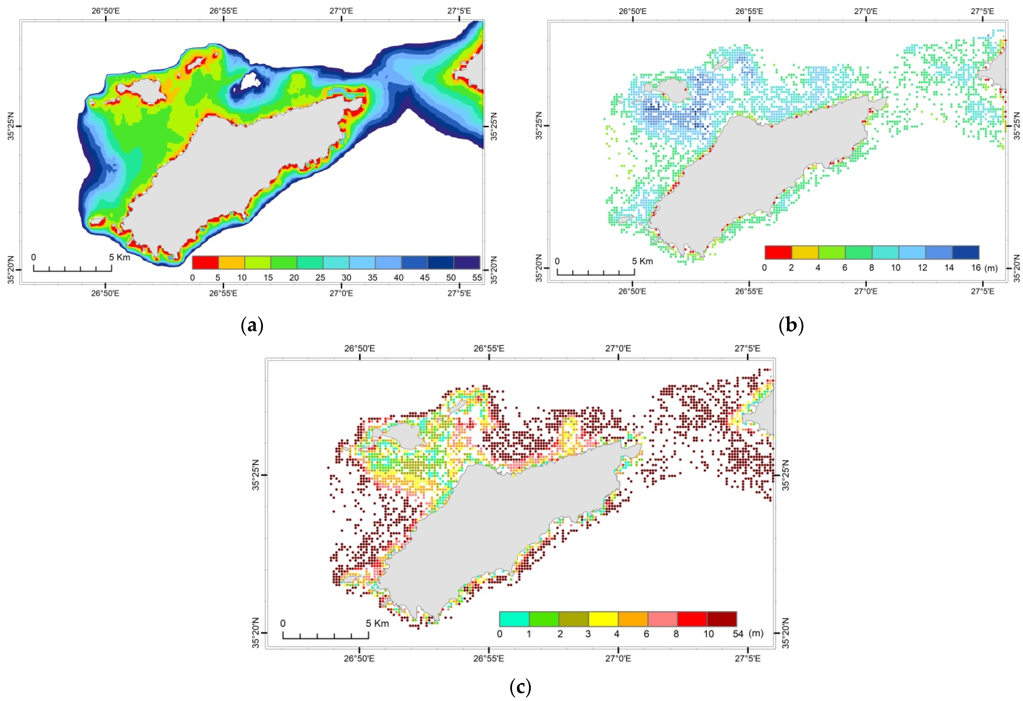
- The reference DTM, concerning the 0–55 m (Figure 7a) and 0–30 m depth zones (Figure 7b), was compared with the analogous Sentinel-2 bathymetric raster images.
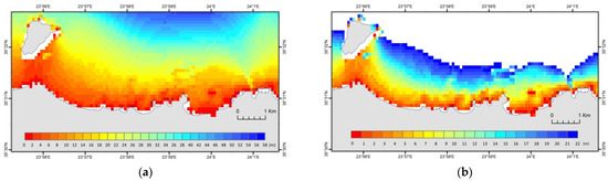 Figure 7. (a) EMODnet DTM of the 0–55 m depth zone for the northwestern coastal area of Crete Island at a resolution of 120 m; (b) The EMODnet DTM spatially adjusted to the Sentinel-2 bathymetric raster image of the 0–30 depth zone.
 - The reference DTM was reprojected and resampled to the resolution (80 m) of the Sentinel-2 DTM to make their comparison appropriate.
- The Sentinel-2 DTM was converted into a vector-point feature and superimposed with the corresponding dataset of the reference DTM (Figure 8a). Depth values for both Sentinel-2 and reference DTM were included in the attribute table of this point feature and, finally, the absolute differences between the two depth fields were calculated. Figure 8b presents the spatial distribution of the absolute values of the above differences, in combination with depth zones defined by the isobath lines (5 m interval) extracted from the reference DTM.
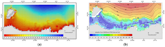 Figure 8. (a) Reference vector-point dataset, having identical extent and resolution with the Sentinel-2 bathymetry; (b) Absolute differences (m) between the two measures. The displayed 5 m interval isobaths were derived from the reference EMODnet DTM.
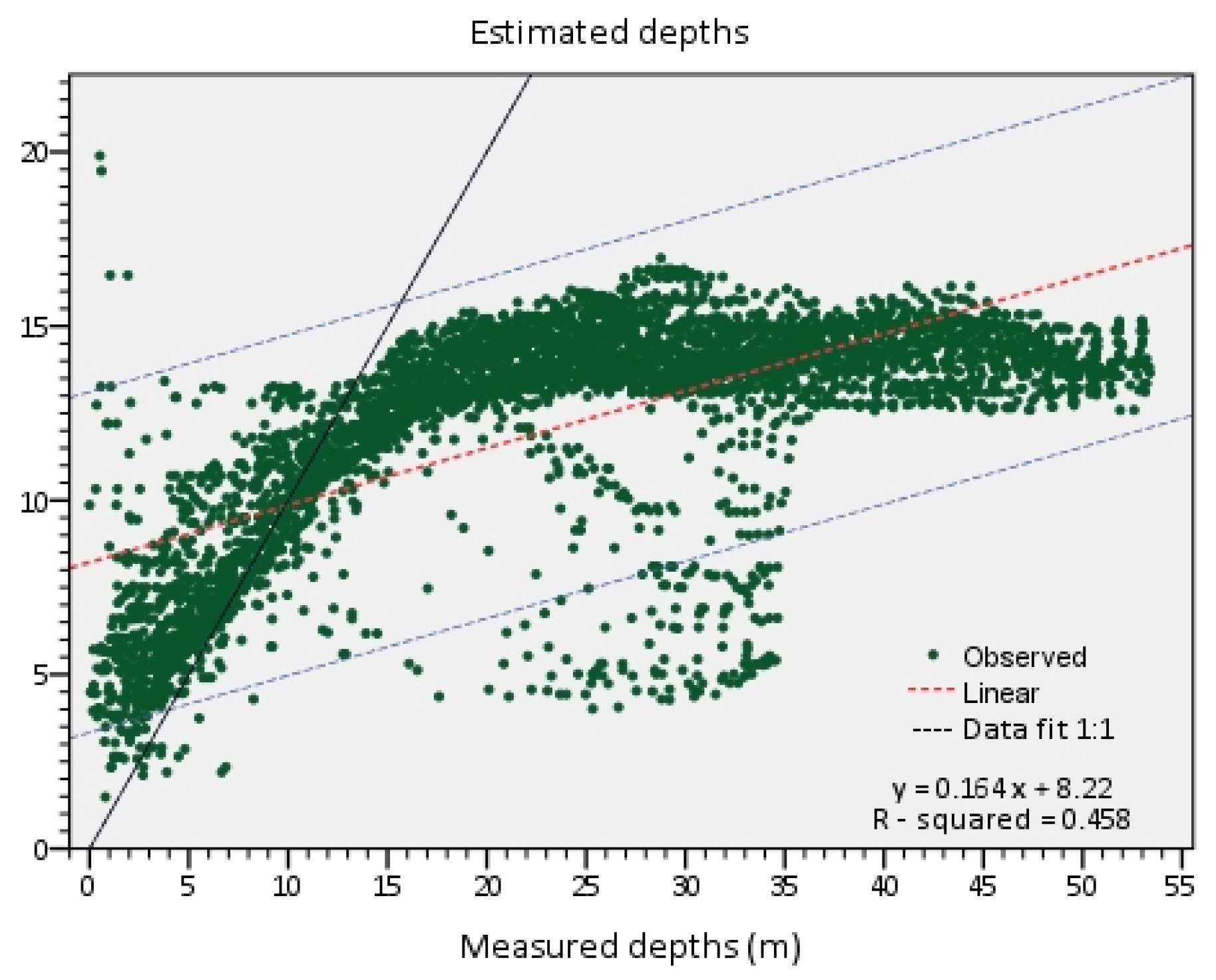
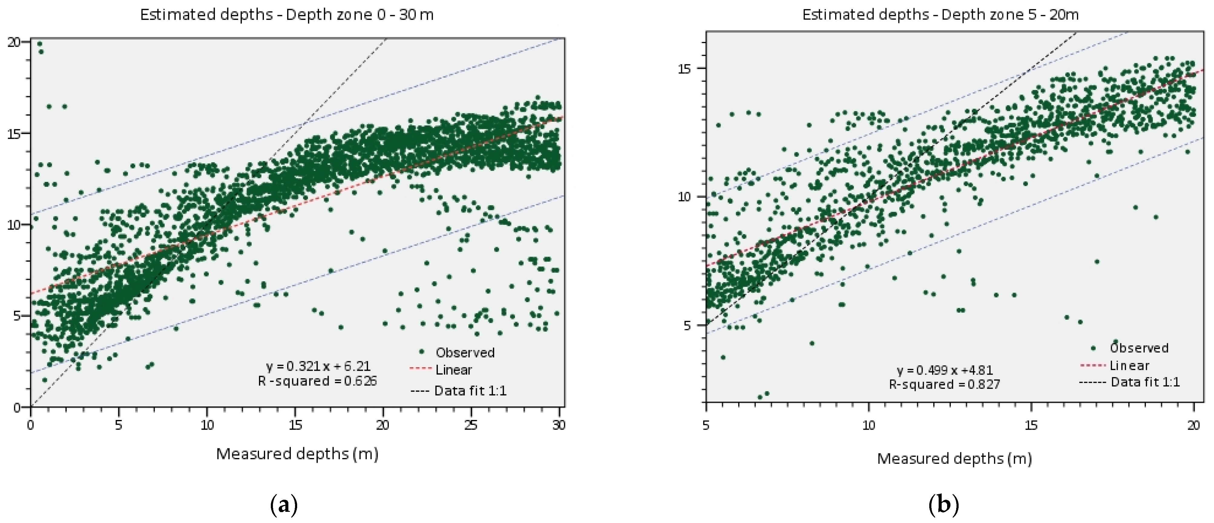
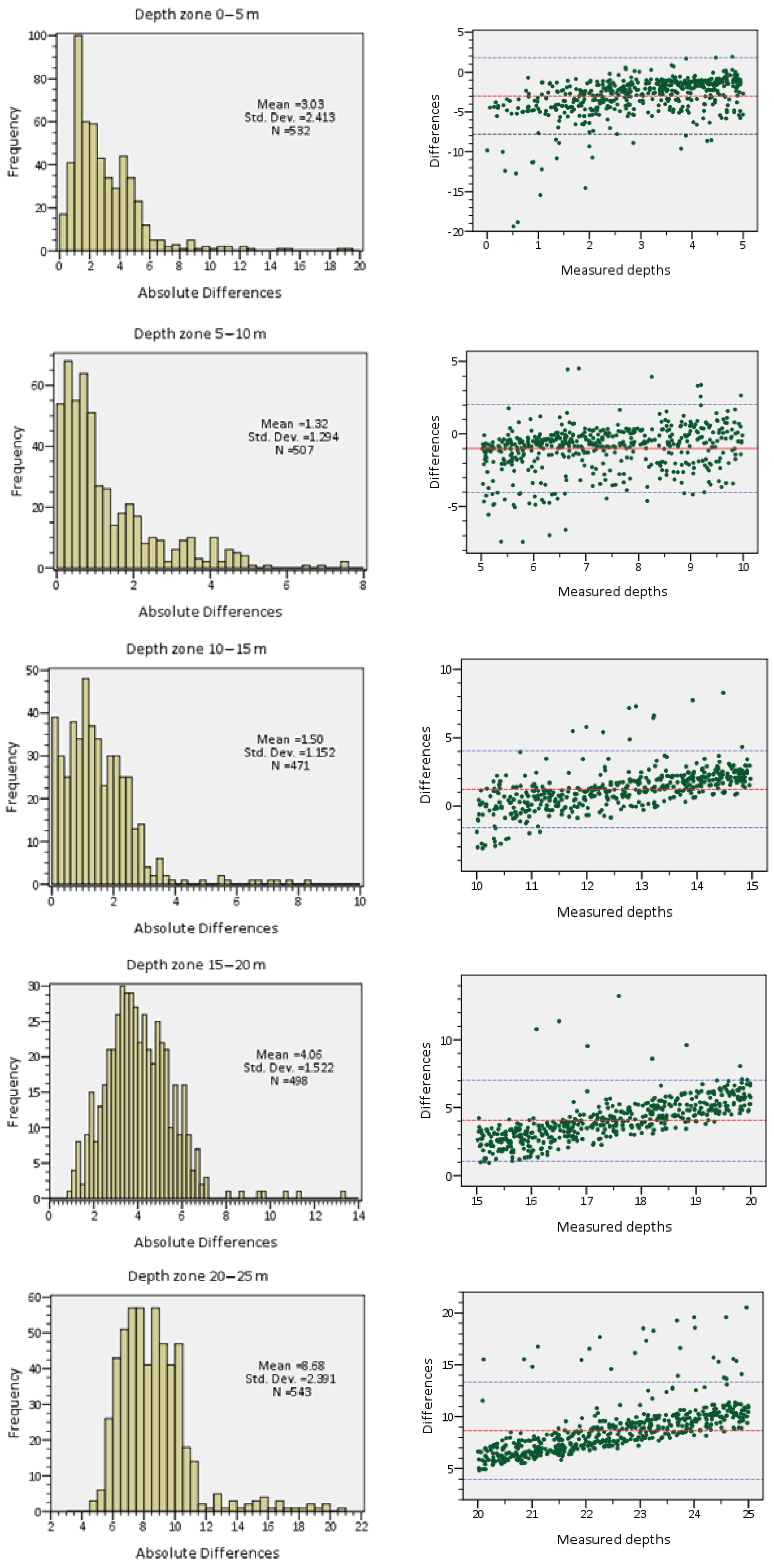
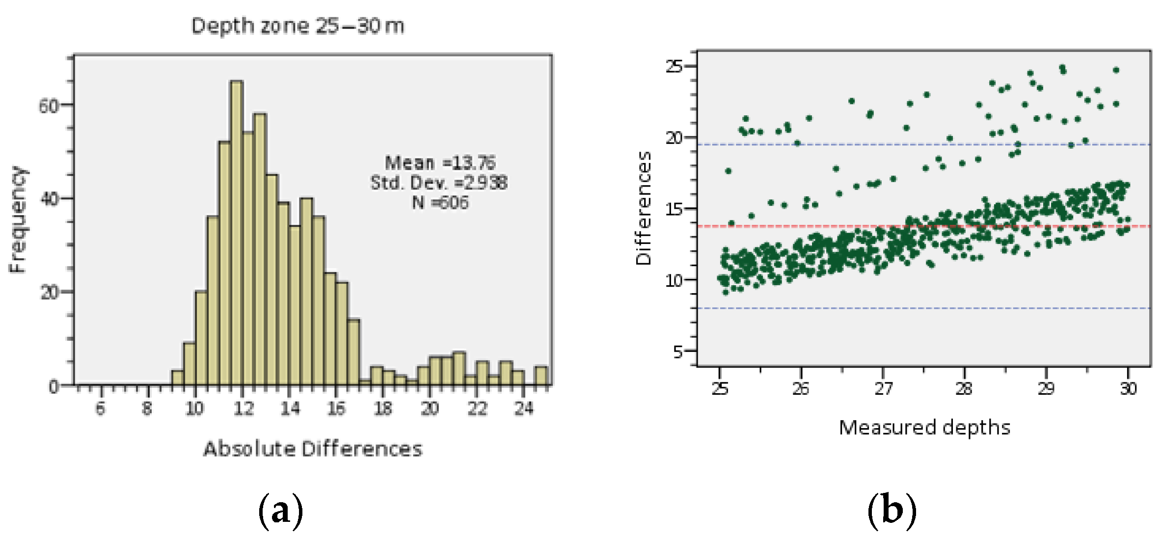
The linear regression applied to the whole study area, i.e., the 0–55 m depth interval, revealed a weak correlation (R2 = 0.458) between the BathySent algorithm results and the reference DTM values (Figure 9), while for the 0–30 m and 5–20 m depth intervals, the linear regression exhibited a stronger correlation (R2 = 0.626 and R2 = 0.827, respectively) (Figure 10). Based on the statistical results presented in Table 1, it is apparent that the BathySent algorithm performed the best within the 5–15 m depth interval, where 75% of the estimated depths demonstrated absolute differences from the reference values lower than 2 m (Figure 11a), while an acceptable result was shown for the 15–20 m depth interval too (see Table 1). In addition, the Bland–Altman plots (Figure 11b), indicated a reasonably good agreement of the two measurement techniques in the 5–20 m depth range, characterized by low mean differences (1–4 m) and an acceptable width of the 95% confidence interval.

Figure 9.
Correlation at the 95% confidence level between the Sentinel-2 bathymetric data and the reference values (0–55 m depth zone).

Figure 10.
(a) Correlation at the 95% confidence level between the Sentinel-2 bathymetric data and the reference values (0–30 m depth zone); (b) Correlation at the 95% confidence level between the Sentinel-2 bathymetric data and the reference values (5–20 m depth zone).

Table 1.
Root Mean Square Error (RMSE) and Mean Absolute Error (MAE) for each depth interval (BathySent results for northwestern coastal area of Crete Island, Cretan Sea).
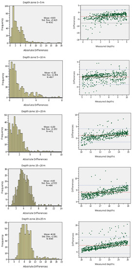
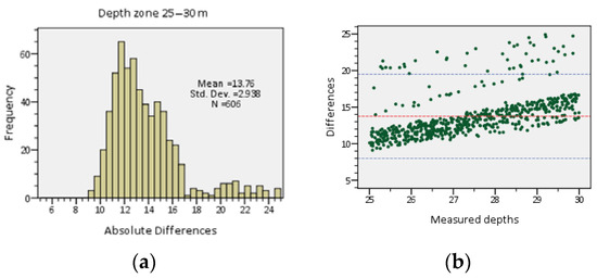
Figure 11.
Depth intervals of 0–5 m, 5–10 m, 10–15 m, 15–20 m, 20–25 m, and 25–30 m: (a) Frequency histograms of the depth differences between the Sentinel-2 bathymetric data and the EMODnet reference bathymetry; (b) Bland–Altman statistical plots assessing the degree of agreement between the two measures, the 95% confidence limits are shown (mean ± (1.96 × st.dev) red and blue lines).
5.3. Kos Island Bathymetric Data Package (DP3)
The DP3 of BathySent bathymetry for the northern coast of Kos Island, derived from the initial Sentinel-2 multispectral data (missions of 2018 and 2019), was originally provided in ENVI format georeferenced to the UTM 35N coordinate system, in double-precision coding, having a spatial resolution of 80 m (Figure 12a) and, then, converted into an ESRI raster geodatabase format (Figure 12b), likewise with the previous DP1 and DP2.
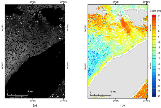
Figure 12.
(a) The initial ENVI format of the depths derived from the BathySent solution applied to Sentinel-2 data (missions of 2018 and 2019) for the northern coast of Kos Island (south Aegean Sea); (b) The output from the application of the BathySent algorithm to the 0–40 m depth zone (80 m resolution).
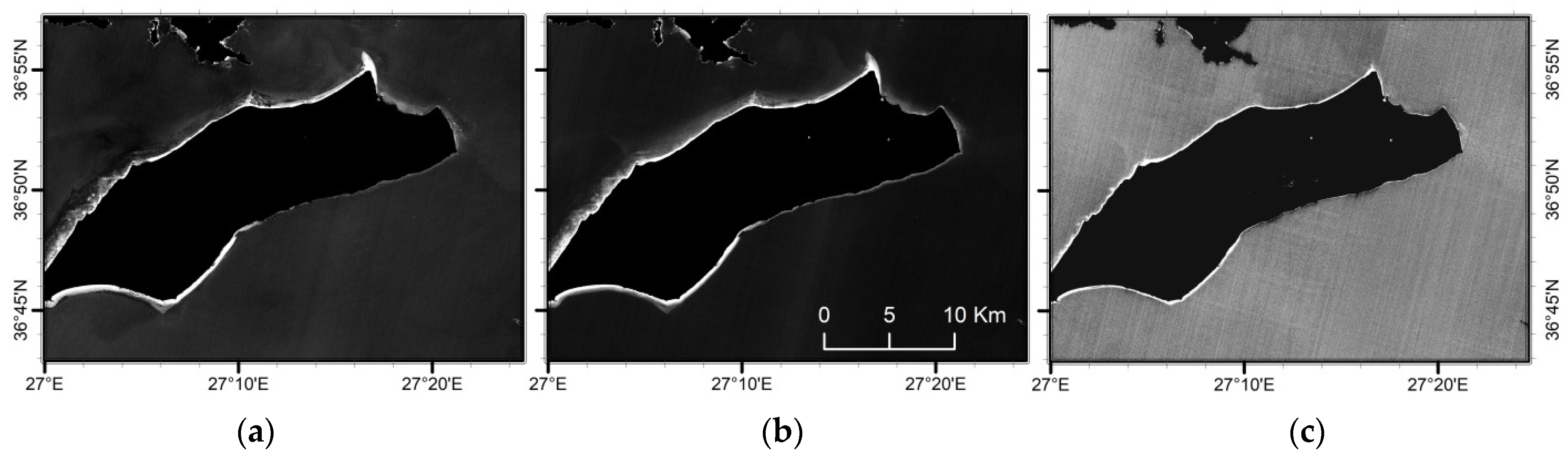
The reference DTM displayed in Figure 13 was resampled to match the resolution (80 m) and extent of the bathymetric raster image derived from the Sentinel-2 data. The latter image was converted into a vector-point dataset, which was compared with the corresponding dataset of the bathymetric survey (Figure 14a). Hence, the differences between the two measurement techniques were calculated (Figure 14b), providing the basis for the subsequent statistical assessment.

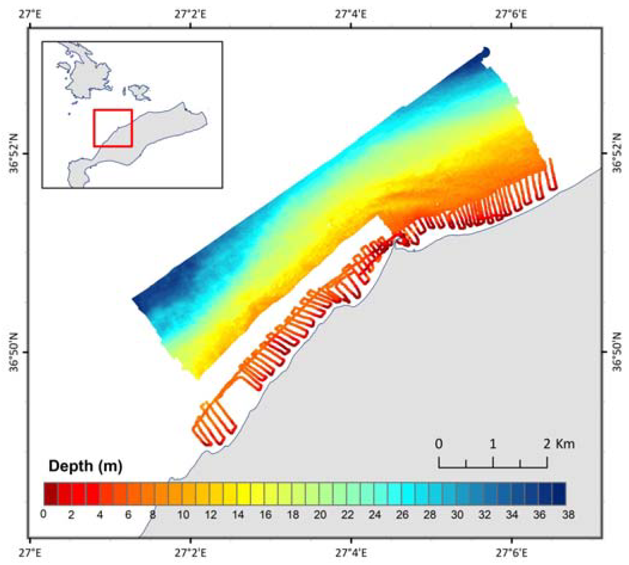
Figure 13.
The surveyed coastal zone north of Kos Island, illustrating the swath bathymetry DTM (grid interval of 2 m) and the single-beam bathymetry tracklines.

Figure 14.
(a) Reference vector-point feature, having identical extent and resolution with the Sentinel-2 bathymetry; (b) Absolute differences (m) between the two measures. The displayed 5 m interval isobaths were derived from the survey data.
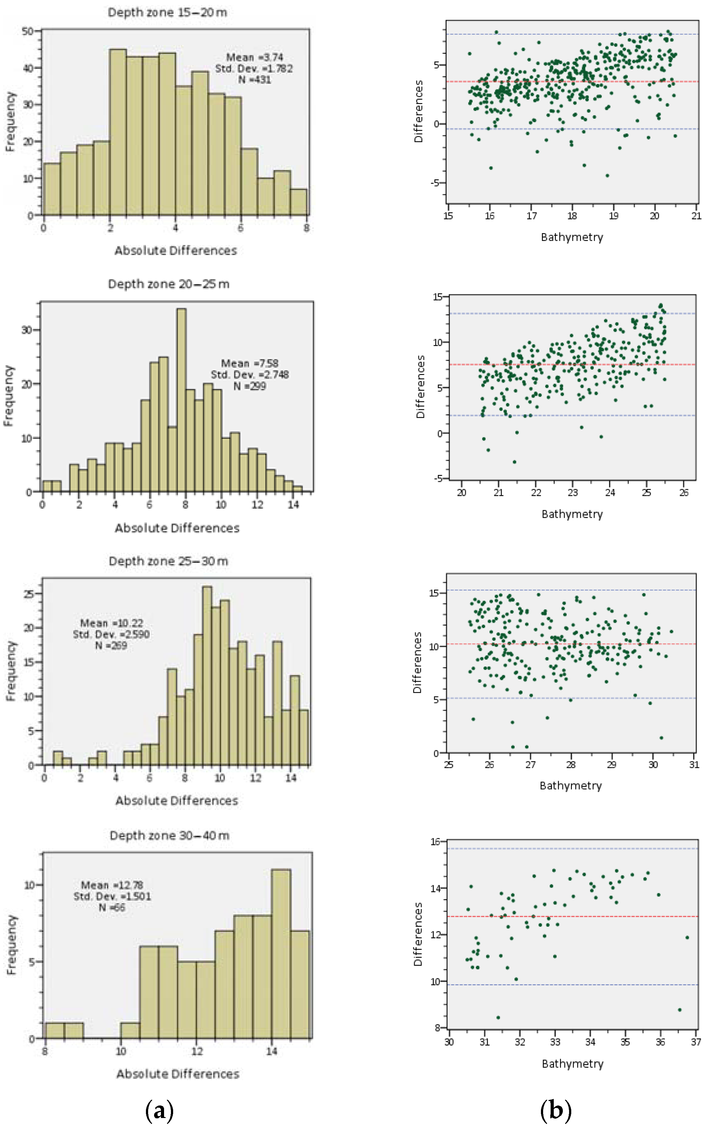
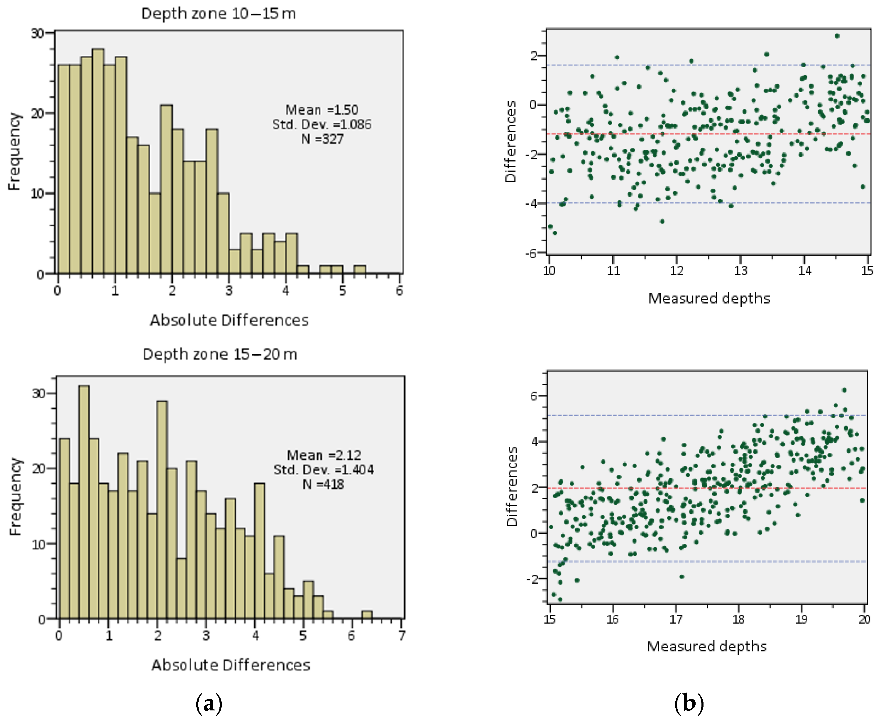
Based on the statistical results presented in Table 2, the BathySent algorithm demonstrated its best performance within the 10–15 m depth interval, showing MAE and RMSE values of 1.58 and 2.41 m, respectively, and 75% of the observations diverging less than 1.9 m from the reference bathymetry. A sufficiently good performance was exhibited for the 5–10 m, 15–20 m, and 20–25 m depth intervals too. For the previous two shallower intervals, 75% of the estimated depths demonstrated absolute differences from the reference values lower than 3.5 and 5 m, respectively (Figure 15a). According to the Bland–Altman plots, the best agreement of the two measurement techniques appeared to occur within the 5–20 m depth range, due to the low mean differences (0–3.5 m) and the acceptable width of the 95% confidence interval (Figure 15b). In contrast, for the 0–5 m depth interval, the BathySent solution provided poor results because 75% of the observations mainly varied from 3.5 to 6 m.
Table 2.
Root Mean Square Error (RMSE) and Mean Absolute Error (MAE) for each depth interval (BathySent results for Kos Island, south Aegean Sea).
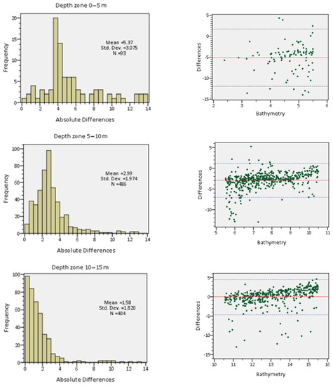
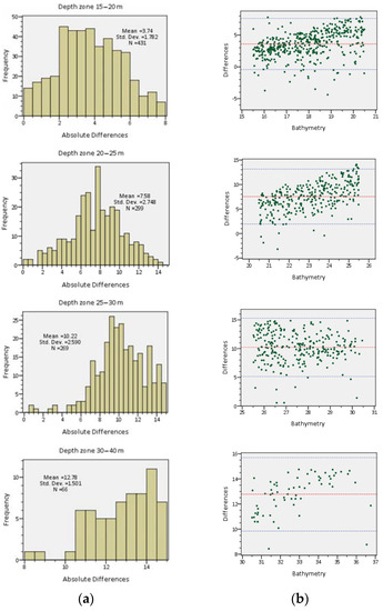
Figure 15.
Depth intervals of 0–5 m, 5–10 m, 10–15 m, 15–20 m, 20–25 m, 25–30 m, and 30–40 m: (a) Frequency histograms of the depth differences between the Sentinel-2 bathymetric data and the survey data; (b) Bland–Altman statistical plots assessing the degree of agreement between the two measures, the 95% confidence limits are shown (mean ± (1.96 × st.dev) red and blue lines).
5.4. Kos Island: Conventional EO-Based Bathymetry Retrieval Approach vs. the BathySent Application to Sentinel-2 Data
For the comparison between the results derived from the performance of a conventional EO-based bathymetry retrieval technique and the proposed innovative BathySent algorithm, using Sentinel-2 data, the Level-1C imagery of Kos Island, obtained from the satellite on 30 September 2019, was downloaded via the Copernicus Open Access Hub. Based on established methodologies, the satellite imagery was corrected for the adjacency effect (or nearby land areas) and atmospheric and sea surface effects. For the elimination of all non-aquatic objects, a ‘water mask’ was created and applied to the image. The atmospheric correction includes the process of removing the contributions of surface glint and atmospheric scattering from the measured total in order to obtain the water-leaving radiance. Hence, the darkest pixel technique and sun glint correction have to be applied.
The darkest pixel technique assumes that there is a high probability that there are at least a few pixels in the image with very low reflectance values, which are assumed to correspond to a black surface with 0% reflectance. The lowest digital number (DN) in each band should actually be zero and, therefore, its radiometric DN represents the atmospheric additive effect [33]. Therefore, the pixels from dark targets are indicators of the amount of the upwelling path radiance and must be removed.
Sun glint, i.e., the specular reflection of light from the water surface, is a crucial confounding factor for the remote sensing of water column properties and benthos, limiting the quantity and accuracy of remotely sensed data. The deglinting method uses Near-Infrared (NIR) spectral data to provide an indication of the amount of glint in the received signal. This is based on the assumption that the water-leaving radiance in this part of the spectrum is negligible and, thus, any NIR signal remaining after the atmospheric correction must be the result of the sun glint. For the aims of this study, the deglinting technique of Hedley et al. [34] was applied, based on the exploitation of the linear relationships between the NIR and the visible bands by using samples of image pixels displaying a range of sun glint. Therefore, image samples were carefully selected and for each visible band, all selected pixels were included in a linear regression of the NIR brightness against the visible band brightness. All image pixels were deglinted (Figure 16) according to the following equation:
where is the deglinted pixel in band i, is the reflectance from the visible band i, is the regression slope, is the NIR band value, and is the minimum NIR value of the sample.
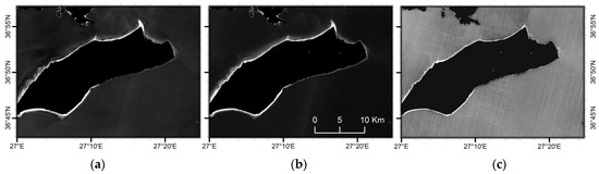
Figure 16.
Atmospherically corrected and deglinted Sentinel-2 bands: (a) Band 2—Blue; (b) Band 3—Green; (c) Band 4—Near-Infrared.
Among the conventional EO-based bathymetry retrieval approaches, the linear ratio model of Stumpf et al. [35] was performed on the atmospherically corrected and deglinted satellite imagery. The model developed by Stumpf et al. [35] considers the fundamental principle that every band has a different level of absorption in the water column. The different levels of absorption will conceptually generate a ratio between bands and this ratio will consistently change simultaneously with water depth variation. The model is expressed by the following equation:
where is the estimated water depth, is a tunable constant defining the slope of the relationship between the band ratio and water depth, and represent the radiance of light reflected off the water surface in the bands i and j (ranging from 1 to 4, i ≠ j), is the offset for zero depth, and, finally, is a constant chosen to assure that the logarithm will be positive under any condition and the band ratio will produce a linear response with water depth change.
Equation (9) actually represents the linear regression between the water depth (dependent variable) and the band ratio (independent variable). For the present study, the ratio of the Blue to Green band was used, while for the definition of the coefficient of regression and model solving, training depth values from the (reference) bathymetric survey in Kos Island were used. Hence, two tests were performed: the first one was carried out for the 0–40 m depth interval and the second one for the 0–20 m depth interval. A set of 120 control points was randomly selected from the reference bathymetry (resampled to 10 m resolution to fit with the satellite imagery resolution) for each depth interval and the relevant regression analyses were run. The results of both analyses are displayed in Table 3 and Table 4.
Table 3.
Model summary for the 0–40 m depth zone.
Table 4.
Model summary for the 0–20 m depth zone.
Based on the shown results, it is evident that the linear ratio model of Stumpf et al. [35] performed better in the 0–20 m depth interval (Figure 17), with the relevant relationship presented in Table 4 being more accurate.
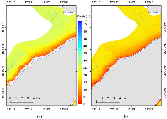
Figure 17.
Bathymetry derived from the linear ratio model of Stumpf et al. [35], based on the equations produced for the 0–40 (a) and 0–20 m (b) depth zones.
The validity of the bathymetric data estimated for the 0–20 m depth interval, using the Stumpf et al. [35] model, was assessed through the random selection of 995 control points (the control points selected for the model calibration were excluded from the assessment) from the ‘pool’ of the reference DTM (resampled to 10 m resolution to fit with the satellite imagery resolution). The MAE, RMSE, and Standard Deviation of the differences in the estimated depths from the measured ones were quite low, being 1.92 m, 2.32 m, and 1.31 m, respectively (see Table 5 and Figure 18a), while a good linear correlation, showing an R2 of 0.71 (Figure 18b), and a good agreement, showing a zero mean difference (Figure 18c), were demonstrated. The R2 value reveals that a major percentage (71%) of the estimated depths can be explained by the Blue:Green ratio of the Stumpf et al. [35] model. Only 30 data points appeared to lie outside the 95% confidence band (Figure 18b), of which 50% referred to the 0–5 m depth interval (Figure 19a). Based on both the low absolute mean difference (1.5–2 m) and relatively limited width of the confidence interval (~6 m) displayed in the Bland–Altman plots of Figure 19b, it seems that the linear ratio model performed better in the 10–20 m depth range.
Table 5.
Root Mean Square Error (RMSE) and Mean Absolute Error (MAE) for each depth interval (ratio model results for Kos Island, south Aegean Sea).
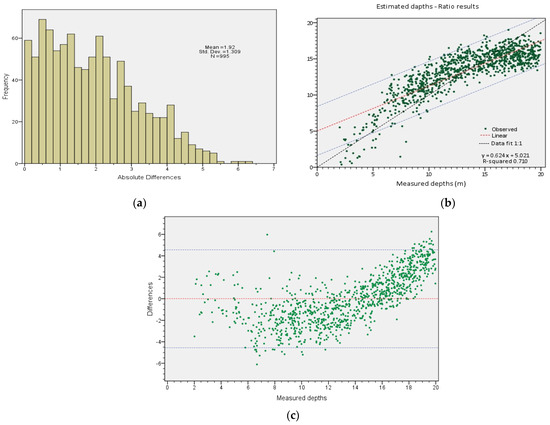
Figure 18.
(a) Frequency histogram of the depth differences between the linear ratio model results and the reference bathymetry; (b) Correlation at the 95% confidence level between the linear ratio model estimates and the reference values (0–20 m depth zone); (c) Bland–Altman statistical plots assessing the degree of agreement between the two measures (the 95% confidence limits are shown, mean ± (1.96 × st.dev) red and blue lines).
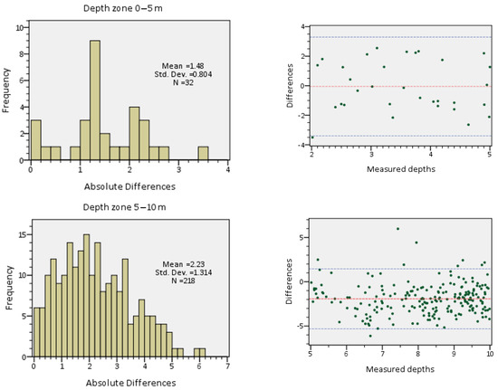
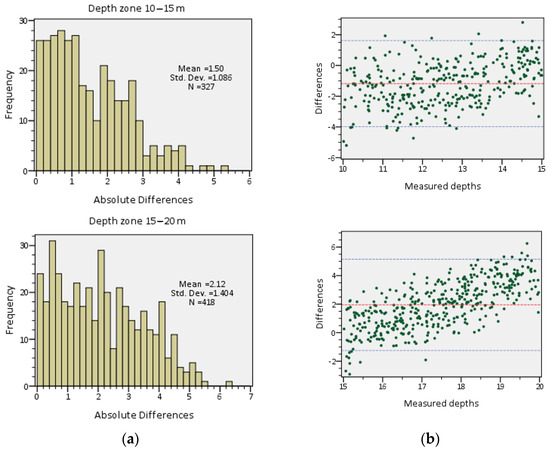
Figure 19.
Depth intervals of 0–5 m, 5–10 m, 10–15 m, and 15–20 m: (a) Frequency histograms of the depth differences between the linear ratio model results and the reference bathymetry; (b) Bland–Altman statistical plots assessing the degree of agreement between the two measures (the 95% confidence limits are shown, mean ± (1.96 × st.dev) red and blue lines).
Finally, in order to compare the efficiency of the BathySent algorithm with the effectiveness of the Stumpf et al. [35] model, the bathymetric output from the latter technique had to be resampled to 80 m resolution to match with the resolution of the output from the BathySent solution for the same study site (see Section 3.3). The absolute differences between the two measurement techniques are displayed in Figure 20. It is evident that within the bathymetric survey area, marked by the red rectangle, the majority of the observations are lower than 2 m, which suggests a good agreement between the two measures. However, the area around 36 degrees 54 min N and 27 degrees 7 min E is where the differences between the two approaches are higher. We found that in this area both the algorithms do not perform very well. On the one hand, the ratio model might be biased because the seawater might not be transparent enough, as it is far from the coasts. On the other hand, waves refracted by the fractal coasts and the presence of sea currents in this area might bias the BathySent solution. A dedicated study on this particular area might be performed in future work. In addition, based on the statistical analysis of the results derived from both techniques, their reliability appears highly enhanced within the 5–20 m depth range, with the linear ratio model output showing a tighter fit. However, the ‘smart’ BathySent solution is a more convenient approach because it does not require any calibration procedure with training depths, which actually offers a valuable benefit to the user.
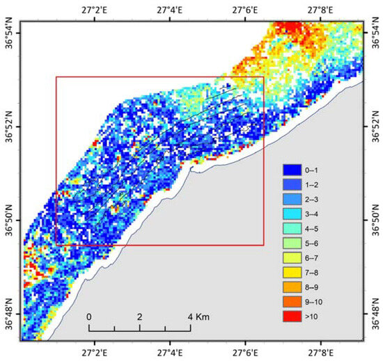
Figure 20.
Absolute differences between a conventional EO-based bathymetry retrieval approach (i.e., the linear ratio model of Stumpf et al. [35]) and the proposed innovative BathySent algorithm, using a Level-1C Sentinel-2 imagery over the pilot study site in Kos Island. The red rectangle includes the (reference) data of the bathymetric survey on Kos Island.
6. Discussion
The proposed algorithm was designed to automatically map coastal bathymetry based on datasets from the Copernicus Sentinel-2 missions. The precision of the retrieved water depths is assessed via their comparison with a variety of reference bathymetric DTMs. The advantage of using Sentinel-2 data lies in the capacity of the satellite’s sensor to cover extensive areas (at national and European scales), while the short satellite revisit period (5 days) is also a great benefit. In addition, the systematic acquisition plan of Sentinel-2 missions is of crucial importance for the monitoring and study of coastal morphodynamics.
The BathySent approach can be applied to all push-broom optical sensors that provide a sufficient time lag between two, or more, spectral bands. As far as our tests are concerned, they definitely can be applied to Landsat 8 and 9. It can be applied to the Spot and Pleiades family of satellites and the future missions CO3D and Pleiades NEO (by the French Space Agency—CNES). We have not yet looked into the SuperDove sensor architecture. In general, we can state that if the sensor architecture is in a matrix form, as opposed to the push-broom architecture, the sensor cannot be used with the BathySent approach.
The BathySent solution, compared to current analogous techniques, is not affected by the occurrence of water turbidity conditions (except in cases of outrageous events) and does not demand field calibration. The major advantages of the BathySent approach are twofold. Firstly, in situ calibration is not needed. Secondly, the dispersion relation (Equation (1)) allows for—theoretical—deeper bathymetry solutions than the ratio-model approach. On the other hand, because BathySent averages c-λ couples over a multi-pixel window, the final bathymetry solution has a lower spatial resolution than that of the ratio-model solution. Our conclusion is that the two methods complement each other. We suggest that they should be used together in a joint inversion, where the BathySent solution is used as a hint to calibrate the ratio-model solution.
Finally, some restrictions and optimization strategies concerning the physical parameters associated with the BathySent algorithm performance are provided below:
- Swell wavelength: The actual resolution of the final output is in the order of the observed wavelength. The theoretical minimum detectable wavelength is twice the pixel size (i.e., 20 m for the Sentinel-2 data). The shorter wavelengths are less sensitive to deeper bathymetry than the larger ones. To improve all previous limitations, an analysis of both short and large wavelengths has to be performed.
- Wave direction: It needs to be adapted to coast geometry. The ideal condition for the wave direction is to be perpendicular to the coastline, but in the case of complex coast geometry, several wave regimes of variable direction have to be used for the analysis of the wave interaction with obstacles.
- Wave visibility: The observed waves must be easily identifiable.
- Water turbidity: The water transparency is a limitation when seabed features are visible in the image, because they can affect the wave celerity estimation. However, extreme surface turbidity may result in patterns with a motion different from the wave motion, which could have an impact on the wave celerity estimation.
- Cloud masking: The presence of clouds, even partially transparent, can affect the wave celerity estimation due to their own motion.
We report a systematic under-estimate of values deeper than 15–20 m, as expected (see [19]). This underestimation is due principally to two factors. In principle, to extract deeper bathymetry, we would need either very large wavelengths or short wavelengths, and a very precise c (precise as 0.01 m/s). Therefore, given that the maximum nominal precision that we can obtain for c is 1/10th of the image pixel size (1 m/s for Sentinel 2), deeper bathymetry values rely on the presence of large wavelengths in the scene. In fact, when we solve Equation (1), if c is overestimated, then h = nan (not a number), whereas if c is underestimated, then h = real but is underestimated. This aspect might be improved in a future research effort.
7. Conclusions
Given the same satellite scene, the maximum water depth retrieved by the BathySent algorithm is lower than the one retrieved by other methods, which determines this parameter based on the swell wavelength. However, the major advantage of the BathySent solution, with respect to all other algorithms, relies on the precise measurement of the wave celerity (not only of the wavelength) and its spatial evolution within the satellite scene. Therefore, the results of the BathySent solution are more robust because they are based on the determination of two physical parameters instead of one.
The assessment of the validity of the BathySent algorithm in three Aegean Sea pilot sites (i.e., islands of Kasos, Kos, and Crete) demonstrated very good results in the 5–25 m depth range, with the solution precision, however, decreasing in deeper depths, ranging from 10 to 30%.
Further, using as a reference the data obtained from a recent bathymetric survey in Kos Island, the linear ratio model of Stumpf et al. [35], and the BathySent algorithm were applied to a Level-1C Sentinel-2 imagery (mission of 2019). The linear ratio model indicated a saturation at ~25 m depth, emphasizing the need for ground calibration. Both techniques provided reliable bathymetry in the 5–20 m depth range (deviations less than 2 m), with the BathySent solution, providing a lower spatial resolution compared to that derived from the ratio linear model. Nevertheless, the absence of a need for in situ calibration of the BathySent algorithm is a great asset and cannot be ignored.
For the successful application of the BathySent solution two critical conditions must be fulfilled:
- The access to the full archive of the Sentinel-2 missions, combining multiple Sentinel-2 acquisitions;
- The occurrence of swell for reliable depth estimates, particularly, at deeper waters. This can be feasible globally, but the local conditions usually play a vital role.
Finally, future developments for the optimum performance of the BathySent algorithm should take into account the following issues:
- Wind-generated waves or currents can affect the precision of the bathymetric retrievals by the BathySent solution, which is primarily based on the imagery of swell waves. Therefore, the proposed algorithm should be further developed in order to automatically select the reliable bathymetries.
- The spatial resolution of the final bathymetric output has to be improved as the FFT window approaches the shallower zone. This issue is critical for the algorithm’s validity and could be addressed by the adaptation of window sizes in a proper interaction scheme.
- To improve the precision of the bathymetric estimates, a combination of multiple sensors, multiple pixel resolutions, and multiple swell regimes should be used (e.g., a combination of Landsat-8, Pleiades, and Sentinel-2 datasets).
Author Contributions
Conceptualization, P.D. and M.d.M.; methodology, M.d.M., D.R., M.F. and P.D.; software, P.D., M.d.M., I.P.P., V.K., D.R., M.F., I.M. and I.L.; validation, P.D., M.d.M. and I.P.P.; formal analysis, M.d.M. and P.D.; investigation, M.d.M., P.D., D.R., M.F., V.K. and D.S.; resources, P.D. and M.d.M.; data curation, P.D., V.K., I.M., I.L., M.d.M., D.R., M.F., D.S. and D.V.; writing—original draft preparation, P.D., I.P.P. and V.K.; writing—review and editing, P.D., I.P.P., M.d.M., V.K. and D.S.; visualization, P.D.; supervision, P.D., M.d.M., V.K. and I.P.P.; project administration, M.d.M. and P.D.; funding acquisition, M.d.M. and P.D. All authors have read and agreed to the published version of the manuscript.
Funding
This research was funded by the European Space Agency (ESA) under the EO Science for Society Permanently Open Call, contract No. 4000124021.
Data Availability Statement
The data that support the findings of this study are available from the corresponding author, upon reasonable request.
Acknowledgments
We are thankful to Espen Volden at ESA. Bathymetric metadata and Digital Terrain Model data products for two (2) of the three (3) pilot sites (Kasos and Crete) were derived from the EMODnet Bathymetry portal—http://www.emodnet-bathymetry.eu (accessed on 14 September 2018), now under the https://emodnet.ec.europa.eu/en/new-emodnet-central-portal (accessed on 20 July 2023). This portal was initiated by the European Commission as part of developing the European Marine Observation and Data Network (EMODNet).
Conflicts of Interest
The authors declare no conflict of interest.
References
- Lyzenga, D.R. Passive Remote Sensing Techniques for Mapping Water Depth and Bottom Features. Appl. Opt. 1978, 17, 379. [Google Scholar] [CrossRef] [PubMed]
- Philpot, W.D. Bathymetric Mapping with Passive Multispectral Imagery. Appl. Opt. 1989, 28, 1569. [Google Scholar] [CrossRef] [PubMed]
- Lafon, V. Methodes de Bathymetrie Satellitale Appliques a l’environnement Cotier: Exemple des Passes d’Arcachon. Ph.D. Thesis, University of Bordeaux 1, Talence, Bordeaux, France, 1999. [Google Scholar]
- Lafon, V.; Froidefond, J.M.; Lahet, F.; Castaing, P. SPOT Shallow Water Bathymetry of a Moderately Turbid Tidal Inlet Based on Field Measurements. Remote Sens. Environ. 2002, 81, 136–148. [Google Scholar] [CrossRef]
- Adler-Golden, S.M.; Acharya, P.K.; Berk, A.; Matthew, M.W.; Gorodetzky, D. Remote Bathymetry of the Littoral Zone from AVIRIS, LASH, and QuickBird Imagery. IEEE Trans. Geosci. Remote Sens. 2005, 43, 337–347. [Google Scholar] [CrossRef]
- Benny, A.H.; Dawson, G.J. Satellite Imagery as an Aid to Bathymetric Charting in the Red Sea. Cartogr. J. 1983, 20, 5–16. [Google Scholar] [CrossRef]
- Bierwirth, P.N.; Lee, T.J.; Burne, R.V. Shallow Sea-Floor Reflectance and Water Depth Derived by Unmixing Multispectral Imagery. Photogramm. Eng. Remote Sens. 1993, 59, 331–338. [Google Scholar]
- Lee, Z.; Carder, K.L.; Chen, R.F.; Peacock, T.G. Properties of the Water Column and Bottom Derived from Airborne Visible Infrared Imaging Spectrometer (AVIRIS) Data. J. Geophys. Res. Ocean. 2001, 106, 11639–11651. [Google Scholar] [CrossRef]
- Sandidge, J.C.; Holyer, R.J. Coastal Bathymetry from Hyperspectral Observations of Water Radiance. Remote Sens. Environ. 1998, 65, 341–352. [Google Scholar] [CrossRef]
- He, J.; Lin, J.; Ma, M.; Liao, X. Mapping Topo-Bathymetry of Transparent Tufa Lakes Using UAV-Based Photogrammetry and RGB Imagery. Geomorphology 2021, 389, 107832. [Google Scholar] [CrossRef]
- He, J.; Lin, J.; Liao, X. Fully-Covered Bathymetry of Clear Tufa Lakes Using UAV-Acquired Overlapping Images and Neural Networks. J. Hydrol. 2022, 615, 128666. [Google Scholar] [CrossRef]
- Irish, J.L.; Lillycrop, W.J. Scanning Laser Mapping of the Coastal Zone: The SHOALS System. ISPRS J. Photogramm. Remote Sens. 1999, 54, 123–129. [Google Scholar] [CrossRef]
- Dalrymple, R.A.; Kennedy, A.B.; Kirby, J.T.; Chen, Q. Determining Depth from Remotely-Sensed Images. In Coastal Engineering 1998; American Society of Civil Engineers: Reston, VA, USA, 1999; pp. 2395–2408. [Google Scholar]
- Leu, L.-G.; Kuo, Y.-Y.; Liu, C.-T. Coastal Bathymetry from the Wave Spectrum of Spot Images. Coast. Eng. J. 1999, 41, 21–41. [Google Scholar] [CrossRef]
- Leu, L.-G.; Chang, H.-W. Remotely Sensing in Detecting the Water Depths and Bed Load of Shallow Waters and Their Changes. Ocean. Eng. 2005, 32, 1174–1198. [Google Scholar] [CrossRef]
- Wu, J.; Juang, J.T. Application of Satellite Images to the Detection of Coastal Topography. Coast. Eng. Proc. 1997, 1, 3762–3769. [Google Scholar]
- Danilo, C.; Melgani, F. Wave Period and Coastal Bathymetry Using Wave Propagation on Optical Images. IEEE Trans. Geosci. Remote Sens. 2016, 54, 6307–6319. [Google Scholar] [CrossRef]
- Poupardin, A.; Idier, D.; de Michele, M.; Raucoules, D. Water Depth Inversion From a Single SPOT-5 Dataset. IEEE Trans. Geosci. Remote Sens. 2016, 54, 2329–2342. [Google Scholar] [CrossRef]
- de Michele, M.; Raucoules, D.; Idier, D.; Smai, F.; Foumelis, M. Shallow Bathymetry from Multiple Sentinel 2 Images via the Joint Estimation of Wave Celerity and Wavelength. Remote Sens. 2021, 13, 2149. [Google Scholar] [CrossRef]
- Abileah, R. Mapping Shallow Water Depth from Satellite. In Proceedings of the ASPRS Annual Conference, Reno Nevada, NV, USA, 1–5 May 2006; pp. 1–7. [Google Scholar]
- Mancini, S.; Olsen, R.C.; Abileah, R.; Lee, K.R. Automating Nearshore Bathymetry Extraction from Wave Motion in Satellite Optical Imagery. In Algorithms and Technologies for Multispectral, Hyperspectral, and Ultraspectral Imagery XVIII; Shen, S.S., Lewis, P.E., Eds.; SPIE: Bellingham, WA, USA, 2012; p. 83900P. [Google Scholar]
- de Michele, M.; Leprince, S.; Thiébot, J.; Raucoules, D.; Binet, R. Direct Measurement of Ocean Waves Velocity Field from a Single SPOT-5 Dataset. Remote Sens. Environ. 2012, 119, 266–271. [Google Scholar] [CrossRef]
- Danilo, C.; Binet, R. Bathymetry Estimation from Wave Motion with Optical Imagery: Influence of Acquisition Parameters. In Proceedings of the 2013 MTS/IEEE OCEANS-Bergen, Bergen, Norway, 10–14 June 2013; pp. 1–5. [Google Scholar]
- Poupardin, A.; de Michele, M.; Raucoules, D.; Idier, D. Water Depth Inversion from Satellite Dataset. In Proceedings of the 2014 IEEE Geoscience and Remote Sensing Symposium, Quebec City, QC, Canada, 13–18 July 2014; pp. 2277–2280. [Google Scholar]
- Abileah, R. Mapping near Shore Bathymetry Using Wave Kinematics in a Time Series of WorldView-2 Satellite Images. In Proceedings of the 2013 IEEE International Geoscience and Remote Sensing Symposium-IGARSS, Melbourne, VIC, Australia, 21–26 July 2013; pp. 2274–2277. [Google Scholar]
- Bergsma, E.W.J.; Almar, R.; Maisongrande, P. Radon-Augmented Sentinel-2 Satellite Imagery to Derive Wave-Patterns and Regional Bathymetry. Remote Sens. 2019, 11, 1918. [Google Scholar] [CrossRef]
- Almar, R.; Bergsma, E.W.J.; Maisongrande, P.; de Almeida, L.P.M. Wave-Derived Coastal Bathymetry from Satellite Video Imagery: A Showcase with Pleiades Persistent Mode. Remote Sens. Environ. 2019, 231, 111263. [Google Scholar] [CrossRef]
- Kudryavtsev, V.; Yurovskaya, M.; Chapron, B.; Collard, F.; Donlon, C. Sun Glitter Imagery of Ocean Surface Waves. Part 1: Directional Spectrum Retrieval and Validation. J. Geophys. Res. Ocean. 2017, 122, 1369–1383. [Google Scholar] [CrossRef]
- Kudryavtsev, V.; Yurovskaya, M.; Chapron, B.; Collard, F.; Donlon, C. Sun Glitter Imagery of Surface Waves. Part 2: Waves Transformation on Ocean Currents. J. Geophys. Res. Ocean. 2017, 122, 1384–1399. [Google Scholar] [CrossRef]
- Bland, J.M.; Altman, D.G. Statistical Methods for Assessing Agreement Between Two Methods of Clinical Measurment. Lancet 1986, 327, 307–310. [Google Scholar] [CrossRef]
- Bland, J.M.; Altman, D.G. Comparing Methods of Measurement: Why Plotting Difference against Standard Method Is Misleading. Lancet 1995, 346, 1085–1087. [Google Scholar] [CrossRef] [PubMed]
- Bland, J.M.; Altman, D.G. Measuring Agreement in Method Comparison Studies. Stat. Methods Med. Res. 1999, 8, 135–160. [Google Scholar] [CrossRef]
- Chavez, P.S. An Improved Dark-Object Subtraction Technique for Atmospheric Scattering Correction of Multispectral Data. Remote Sens. Environ. 1988, 24, 459–479. [Google Scholar] [CrossRef]
- Hedley, J.D.; Harborne, A.R.; Mumby, P.J. Technical Note: Simple and Robust Removal of Sun Glint for Mapping Shallow-water Benthos. Int. J. Remote Sens. 2005, 26, 2107–2112. [Google Scholar] [CrossRef]
- Stumpf, R.P.; Holderied, K.; Sinclair, M. Determination of Water Depth with High-Resolution Satellite Imagery over Variable Bottom Types. Limnol. Oceanogr. 2003, 48, 547–556. [Google Scholar] [CrossRef]


Disclaimer/Publisher’s Note: The statements, opinions and data contained in all publications are solely those of the individual author(s) and contributor(s) and not of MDPI and/or the editor(s). MDPI and/or the editor(s) disclaim responsibility for any injury to people or property resulting from any ideas, methods, instructions or products referred to in the content. |
© 2023 by the authors. Licensee MDPI, Basel, Switzerland. This article is an open access article distributed under the terms and conditions of the Creative Commons Attribution (CC BY) license (https://creativecommons.org/licenses/by/4.0/).