Assessment of Hydrological Response to Climatic Variables over the Hindu Kush Mountains, South Asia

Abstract

The impact of climate extremes, such as heat waves and extreme rainfall, can cause harvest failures, flooding, and droughts that ultimately threaten global food security, harming the region’s economy. Fluctuations in streamflow indicate the sensitivity of streamflow responding to extreme precipitation events and other climatic variables (temperature extremes) that play a significant role in its generation. Pakistan is also considered one of the climate change hotspot regions in the world. The devastating impacts have often occurred in recent decades due to an excess or shortage of streamflow, majorly generated from the Upper Indus Basin (UIB). To better understand climate extremes’ impact on streamflow, this study examined climate extremes and streamflow (Q) changes for three decades: 1990–1999, 2000–2009, and 2010–2019. Observed streamflow and meteorological data from nine sub-catchments across all climatic zones of the UIB were analyzed using RGui (R language coding program) and partial least squares regression (PLSR). Climatic variables were estimated, including precipitation extremes, temperature extremes, and potential evapotranspiration. The Mann–Kendal test was applied to the climatic indices, revealing that precipitation increased during the last 30 years, while maximum and minimum temperatures during the summer months decreased in the Karakoram region from 1990 to 2019. The spatiotemporal trend of consecutive dry days (CDD) indicated a more increasing tendency from 1990 to 2019, compared to the consecutive wet days (CWD), which showed a decreasing trend. PLSR was applied to assess the relation between climatic variables (extreme P, T indices, and evapotranspiration). It was found that the dominant climatic variables controlling annual streamflow include the r95p (very wet days) and R25mm (heavy precipitation days), maximum precipitation event amount, CWD, PRCPTOT (annual total precipitation), and RX5 (maximum five-day precipitation). The TXn (Min Tmax) and Tmax mean (average maximum temperature) dominate streamflow variables. Moreover, the impact of evapotranspiration (ET) on variations in streamflow is more pronounced in arid catchments. Precipitation is the predominant factor influencing streamflow generation in the UIB, followed by temperature. From streamflow quantification, it was found that climate-driven annual streamflow decreased during 1999–2019 in comparison to 1990–1999, with an increase in a few catchments like Kalam, which increased by about 3.94% from 2000 to 2010 and 10.30% from 2010 to 2019, and Shigar, which increased by 0.48% from 2000 to 2009 and 37.37% from 2010 to 2019 concerning 1990–1999. These variations were due to changes in these climatic parameters. The PLSR approach enables the identification of linkages between climatic variables and streamflow variability and the prediction of climate-driven floods. This study contributes to an enhanced identification and hydroclimatological trends and projections.

1. Introduction

The variation in a streamflow reveals how responsive it is to rainfall extremes and the many roles climate factors play in generating streamflow [1,2,3,4]. Floods caused by precipitation extremes typically make up a large streamflow but have numerous adverse effects on human life and the environment at the catchment level, especially in arid and semiarid regions [5,6,7]. Several watershed management initiatives or hydrologic constructions were performed globally to lessen these adverse effects, resulting in alterations to streamflow [5,6]. While more noticeable variations in precipitation extremes have been seen as a result of altering geographical and meteorological conditions, mixed patterns of changes in precipitation have also been identified in the context of climate change [8,9,10,11,12] More intense extreme precipitation events have the potential to lead to more severe flooding and sediment erosion, which would exacerbate these adverse effects [13]. To create more effective watershed management strategies and assess streamflow changes, stakeholders must understand the links between climate factors and streamflow generation. High-highland Asia is largely covered by the Upper Indus Basin (UIB). For Pakistan’s well-being, its water resources are of the utmost importance. Pakistan relies primarily on water from the Indus and its tributaries for household use, agricultural, and hydroelectric needs [14,15]. Agricultural output from irrigated land in the Indus Basin supplies 85% of the country’s cereal grain (wheat, rice) harvests and all of its sugar production, and it employs 45% of Pakistan’s workforce. Additionally, the region is significant for hydropower production; the Tarbela Dam alone meets almost 20% of the country’s electricity needs. Pakistan’s issues with food security and electricity load shedding would be far worse without the contribution of the Indus River, which is regarded as the country’s lifeline. The UIB’s current water resource management issues are principally brought on by the wide interannual variation in river flows and the timing of the hydrograph’s rising limb. Water stress in Pakistan is primarily caused by high population growth in the future. Still, hydroclimatological variability will make it more difficult to manage resources because acute conditions in dry, low-flow years may overwhelm adaptation measures designed to deal with mean changes in water availability [14].

According to several studies, the atmosphere in India has warmed up [16,17,18,19]. Shrestha et al. [19] found increases in winter maximum temperatures of 0.61, 0.90, and 1.24 °C decade-1 for the Nepal, Himalayan, and trans-Himalayan climatic sites, respectively. According to [20], Pakistan’s temperature is expected to rise by 0.9 °C by 2020 and could double by 2050. It was claimed that China’s temperatures were trending up, whereas high-latitude areas during the summer were trending down. The southwest regions of Xinjiang and Tibet have shown a warming trend throughout the wintertime [2,20,21]. Fowler et al. [22] used regression techniques to analyze temperature data from seven climate stations in the Hindu Kush and Karakoram mountains from 1961 to 1999. They discovered a tendency toward winter warming and summer cooling. Research on precipitation trends has also been conducted in South Asia [23]. Gemmer et al. [24] showed a rising precipitation trend between 1951 and 2002 in southern Xinjiang, which is close to Pakistan’s northern border, and in Jammu and Kashmir, southwest of Tibet. Using linear regression, Archer et al. [14] examined precipitation data from numerous locations in the upper Indus River basin with varied record durations. Between 1961 and 1999, a discernible upward trend in precipitation was particularly pronounced in the winter and summer [24,25].

On the contrary, Raziei et al. [26] concluded that precipitation in Iran is decreasing. Kezer et al. [27] looked at runoff patterns for the Ili and East Rivers in Central Asia; no statistically significant change was found besides runoff. Chen et al. [28] used the Mann–Kendall test and linear regression to evaluate temporal (1951–2003) patterns in annual and seasonal precipitation, temperature, and runoff in the Hanjiang basin in China. The results showed that while temperature significantly increased throughout most of the basin at the 5% level, precipitation did not significantly increase [20,29,30]. Additionally, the Danjiangkou reservoir basin’s mean annual, spring, and winter runoffs declined. The South Asian area is undoubtedly warming, and the trajectory of warming is generally comparable with the global warming trend, according to the findings of various recent research [17]. As a result, the South Asian area is expected to see significant climatic effects on many parts of the natural environment, including water supplies. According to the most current Intergovernmental Panel on Climate Change (IPCC) [31,32], there is a strong possibility that South Asian subregions could warm significantly, with winter warming expected to be larger than summer warming. The average temperature is predicted to rise throughout South Asia under the results of a multimodal global climate model (GCM) run under the Special Report on Emission Scenarios (SRES) B1 and A1F1. The highest increase is predicted during the winter months. The expected temperature increase for the winter months is higher than the [33] estimated range of global mean surface temperature change (1.8 to 4 °C). Much research has been conducted on how the changing climate may affect hydrological systems [33].

Assessment of the effects of climate change in basins with a snow-dominated environment has been the topic of several recent publications. Refs. [34,35] studied how the timing of spring runoff in West-Central Canada has been affected by climate change. In northern Canada’s Liard and Mackenzie River basins, and Ref. [36] looked at trends and variability in hydrological variables for natural streamflow gauging stations. Both basins exhibited an increase in winter flows and some increases in spring runoff. Aziz et al. [37] noted an earlier onset of the spring freshet over the Mackenzie River basin. Novotny et al. [38] reported that in Minnesota’s five main river basins, the potential for floods has grown due to rainfall events rather than snowmelt. Climate change may add to the already heavy strain that urbanization, industrialization, and economic expansion have placed on ecological and social systems in emerging nations like Pakistan. With its large and growing population and an economy closely tied to its natural resource base, Pakistan is highly vulnerable to the effects of climate change. Recent research from the South Asian area indicates that hazards to human water security or biodiversity are becoming frequent [39]. According to the International Centre for Integrated Mountain Development (ICIMOD), there are more than 12,000 glaciers in the Himalayan area, and the Indus River is refilled by meltwater from about 3300 glaciers [40]. Changes in water’s temporal and spatial distribution are anticipated to affect Pakistan’s water security. Due to changes in the hydrological cycle’s dynamics, the unpredictable and unclear water supply pattern is expected to affect agricultural production. Since the functioning of ecosystems, economic activity, human health, and geophysical processes have all depended on the availability of that water [41,42]. An evaluation of ER’s and climatic variability’s effects on streamflow variations within the UIB has emerged as a critical area of study. In climate change and human disturbances, several models have recently been created to examine the relationships between climatic variables and streamflow generation (Milly). However, the typical characteristics of hydrological models include complex model structures, many input datasets and parameters, and a significant amount of time and uncertainty needed for model calibration and assessment [43]. As a result, empirical models based on methods like multiple linear regression [44,45] principal component analysis, autoregressive moving average time-series modeling, artificial neural networks, genetic programming, and support vector machines are frequently used to quantify the effects of climatic variables on streamflow [46,47,48,49]. Using data with strong correlations among variables disrupts the model’s expected data patterns, causing the model’s assumptions to be invalid. This leads to inaccurate estimates for model parameters and broader or narrower confidence intervals, undermining the model’s reliability in making predictions [50,51]. As a result, it is crucial to use caution when connecting climatic factors to hydrological processes [52].

Furthermore, it is challenging to identify the primary mechanisms regulating streamflow in regional catchments since addressing multi-collinearity and noise is a challenge for standard techniques to model construction. The recently created and extensively used partial least squares regression (PLSR) method offers an alternate strategy to get beyond the issues with multi-collinearity and noise, permitting more accurate abstraction of the key variables influencing streamflow [37,40]. PLSR generalizes both principal component analysis and multiple linear regression by combining their characteristics [53]. It recognizes underlying model structures that entail linear combinations of the original variables and clarifies the existence of variable dependency [50,53]. Another characteristic of PLSR is its suitability when the number of potential variables is equal to or greater than the number of observations [54,55].

This research aims to address a critical research gap concerning the impact of climate extremes on streamflow in the Upper Indus Basin (UIB), a region susceptible to climate change. The growing concerns about global food security and the severe consequences of climate extremes, such as heatwaves, extreme rainfall, floods, and droughts, underscore the urgency of understanding how these climatic events affect streamflow, which is vital for water resource management and agriculture in the UIB. Despite being recognized as a climate change hotspot, there is a shortage of comprehensive studies on the relationships between climate extremes and streamflow in this region. This research employs a multi-decade streamflow and meteorological data analysis, utilizing advanced statistical techniques like PLSR to discern the intricate connections between climatic variables and streamflow variations. By identifying the dominant climatic factors influencing streamflow and quantifying the changes in climate-driven streamflow over time, this study seeks to contribute significantly to the knowledge of hydroclimatological trends and predictions in the UIB, ultimately assisting in better water resource management and adaptation strategies for this vulnerable region. This study uses PLSR to examine the connections between annual streamflow and climatic variables, particularly extremes in precipitation, in the Loess Plateau (LP) from 1961 to 2015. Given that the two ecological restoration (ER) techniques result in different streamflow regime changes, the effects of climatic variation and ER, in particular, were assessed on streamflow in the LP over the two ER periods [56]. The specific goals are to (1) estimate different precipitation extremes and other meteorological factors and (2) determine the climatic factors that dominate streamflow generation and measuring streamflow change.

2. Materials and Methods

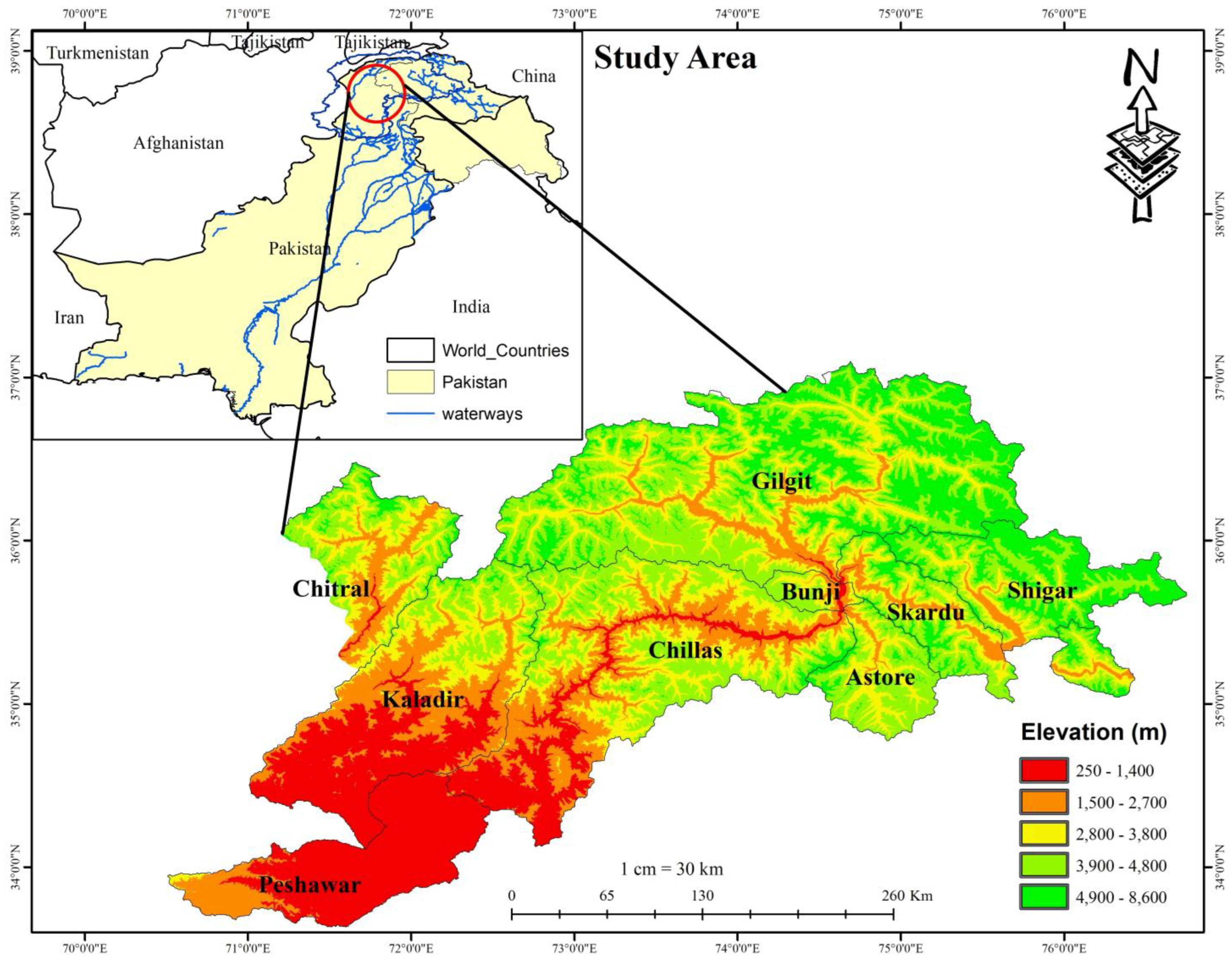
2.1. Study Area

The area for this research is the UIB in Pakistan. It covers the province of Khyber Pakhtunkhwa, the Gilgit-Baltistan area, and some portions of Punjab. This covers a sizable section of Pakistan’s most northern regions. Geographically, the UIB is found between latitudes of about 35° and 37° N and longitudes of around 72° and 77° E. Rugged mountain ranges, broad valleys, and tall plateaus characterize the region. It is divided into sub-catchments that provide water to the entire basin, as shown in Figure 1. Elevation ranges from almost 1500 m (4900 feet) in the valleys to 8000 m (26,000 feet) at the highest peaks.

The Indus River passes through many landscapes, links various areas, and supplies vital water resources to millions of people in Pakistan, which has enormous geographic significance. The UIB has a variety of climatic conditions. As a result, the UIB’s sub-basins respond to various climatic variables in diverse ways. The primary sources of streamflow for sub-basins in high-altitude areas having lots of glaciers and snow cover are more dependent on snowmelt and glacier melt. Sub-basins in lower-altitude regions could be more affected by monsoonal rainfall. The monsoon season’s timing, severity, and duration can impact streamflow patterns in these areas.

The Indus River, generated through the UIB, is given a lot of attention in Pakistan. An essential piece of infrastructure, the Tarbela Hydropower Dam in Pakistan harnesses the power of the Indus River to produce electricity. It is one of the world’s biggest earthen dams and is essential to Pakistan’s energy industry. It uses the Indus River’s water flow to power turbines, which power generators that generate electricity. Pakistan’s agricultural economy is supported by a vast network of irrigation systems along the Indus River that provide water to large agricultural areas. The Indus River ensures an efficient supply of water for irrigation. Being one of Asia’s most significant water systems, the UIB provides water to the most extensive irrigation system in the world, providing water for 90% of Pakistan’s food production and 25% of the nation’s gross domestic product (GDP) [57]. Figure 2 represents the methodology flow chart of this study.

2.2. Climatological and Hydrological Data

The climatological data, including precipitation P, daily max temperature Tmax, daily min temperature Tmin, wind speed, and relative humidity from 1990 to 2019, were collected from the Pakistan Meteorological Department (PMD). The PMD adheres to all SOPs relating to the instrumentation and collection of data and its distribution to final users. Also, the PMD is a member of the World Meteorological Organization (WMO). The meteorological station details lying in the UIB are given below in

Table 1. List of Meteorological Stations in the UIB.

Sr. No.	Station Name	Longitude (°)	Latitude (°)	Elevation (m)
1	Astore	74.90	35.33	2450
2	Bunji	74.63	35.67	1400
3	Chilas	74.10	35.42	1265
4	Chirtal	71.83	35.85	1494
5	Drosh	71.80	35.56	1360
6	Gilgit	74.33	35.92	1500
7	Gupis	73.44	36.22	2713
8	Hunza	74.65	36.31	2438
9	Peshawar	71.56	34.02	331
10	Cherat	71.88	33.82	892
11	Kalam	72.57	35.49	2001
12	Saidu Sharif	72.35	34.73	970
13	Dir	71.87	35.19	420
14	Shigar	75.69	35.49	2230
15	Skardu	75.55	35.32	2228

.

Data on daily streamflow was obtained from the Surface Water Hydrology Project (SWHP), run by the Water and Power Development Authority (WAPDA) from 1990 to 2019. Streamflow is one of the main parameters that enables researchers to comprehend the fluctuation and movement of water in a streamflow and the flow of water in streams, rivers, and other channels. The hydrological stations’ lying in the UIB details are given below in

Table 2. List of Hydrological Stations in the UIB.

Sr. No.	Station Name	Longitude (°)	Latitude (°)	Area (km2)
1	Astore at Doiyan	74.7	35.5	4040
2	Skardu at Kachura	75.4	35.5	112,665
3	Kalam at Chakdara	34.6	72.0	5776
4	Chitral	71.8	35.9	11,396
5	Indus at Besham Qilla	72.9	34.9	162,393
6	Gilgit at Alam Br.	74.3	35.9	26,159
7	Jhansi Post	71.4	33.8	1257
8	Shigar	75.7	35.4	6610
9	Bunji	74.6	35.7	142,709
10	Indus at Massan	71.7	33.0	286,000

.

2.3. Calculations by Expert Team on Climate Change Detection and Indices (ETCCDI) Climatic Variables Using the RClimDex

The ETCCDI variables are a group of fundamental climate indices that are used to track the occurrence of T and P extremes. Temperature indices concentrate on the cold and warm extremes of the min and max T, including max/min values, fixed threshold exceedances, and percentile-based thresholds. Precipitation indices concentrate on total precipitation accumulations, rainfall occurrences with points, and maximum rainfall extremes. These variables were calculated using the RClimDex, an extension of R 4.3.1 language software. It is a program built by Microsoft Excel that is a simple-to-apply package for calculating indices of climate extremes for identifying and monitoring climate change (CC). A total of 27 indices are calculated by the RClimDex. In this study, 19 essential variables were calculated. From gathering climate data to running the functions that create the index, several processes are involved in producing climate indices with the RClimDex. The RClimDex is a powerful climate analysis tool in R that employs a suite of equations to calculate a wide range of climate indices. These indices are essential for characterizing climate extremes and trends, aiding researchers and climate scientists in understanding historical climate data and assessing the impact of climate change. Some of the equations used within the RClimDex encompass simple daily temperature indices, such as TXx (the maximum temperature on the hottest day), which identifies the highest daily maximum temperature within a specified period. Precipitation indices, including the R1mm (the number of wet days) and Rx1day (maximum 1-day precipitation), are also calculated based on observed daily precipitation records. Additionally, percentile-based indices like the PRCPTOT (precipitation total percentile) and climate extreme indices like the growing season length (GSL) are derived through equations that quantify specific climate characteristics, such as the percentage of total precipitation below a certain threshold and the duration of growing seasons.

Furthermore, the RClimDex provides various tools and equations for assessing climate extremes, including consecutive dry days (CDD), consecutive wet days (CWD), and frost-related indices like GSL25 and GSL5. These equations collectively enable users to examine various facets of climate behavior, helping to unravel historical climate patterns and detect trends and anomalies driven by climate change. By employing these equations and indices, the RClimDex empowers researchers to conduct comprehensive climate analysis and generate critical insights into climatic variability and change.

2.4. Evapotranspiration Calculation

The Penman–Monteith equation was employed in this study to determine evapotranspiration. The equation is an empirical method for calculating the rate of evapotranspiration, which is the total amount of water lost to the atmosphere due to land surface evaporation and plant transpiration. The equation is expressed as the following:

$$ET=(0.408\Delta (Rn-G)+\gamma (900/(T+273)u^2(es-ea)/(\Delta +\gamma (1+0.34u^2\left)\right)$$

(1)

where E is the rate of evapotranspiration (mm/day), Rn is the net radiation (MJ/m²/day), G is soil heat flux density (MJ/m²/day), γ is the psychometric constant (kPa °C⁻¹), T is the air T in degrees Celsius (°C), u² is the speed of wind at 2 m above the ground in meters per second, es is saturation VP in (kPa), ea is actual VP (kPa), and Δ is the saturation vapor pressure–temperature curve’s slope (kPa/°C).

2.5. Spatial Analysis by Inverse Distance Weighting (IDW)

Spatial analysis, also known as spatial data analysis, is a clearly defined subset of the analytical techniques that can be used in a project. If the data are spatial, or when they are referred to as a 2-dimensional frame, one may describe spatial analysis as a collection of techniques [58]. In this study, the IDW tool from the Geographic Information System (GIS) is applied for the spatial analysis of climatic variables. Interpolation is performed using the IDW method. The fundamental presumption behind it is that the attribute value of an unsampled point is the weighted average of all known values in the immediate vicinity. Using values from a dispersed set of known points, unknown facts are given importance in this procedure [59,60,61,62,63,64,65,66]. The basic equation of IDW is the following:

$$P=\sum (Pi/D{i}^n)/\sum (1/D{i}^n)$$

(2)

where P represents the estimated value for the unknown place, Pi is the known value at each point i, Di is the distance from the undisclosed location to each available site i, and n is a power parameter that controls the significance of known points on the interpolated values based on their distance to the unknown end.

2.6. Trend Analysis

Trend analysis is a statistical method used to spot patterns or trends over a predetermined timeframe. To determine whether a group of data values is increasing over time or dropping with time, the Mann–Kendall (MK) test was utilized and found if the trend of climatic variables over the UIB, in either direction, was increasing or decreasing.

Mann–Kendall Test

The MK test, often called the Mann–Kendall trend test, is a popular non-parametric statistical tool for examining trends in time-series data. In 1945, Mann made the initial suggestion, and in 1975, Kendall expanded on it. The MK test determines whether the trend of the relevant variable over time is upward or downward. An upward trend, which may or may not be linear, denotes a constant growth in the variable over time [60]. General Equations (3)–(6) represent the method:

$$S={\sum }_{k=1}^{n-1}{\sum }_{j=k+1}^{n}sgn(X_j-X_k)$$

(3)

The p-value must be determined. When the estimated probability is below that significance level, the null hypothesis of no trend is rejected. To achieve this, we must first use the VAR(S) to determine the value of z.

$$VAR(S)=\frac{n(n-1)(2n+5)-\sum _{i=1}^{n}ti(ti-1)(2i+5)}{18}$$

(4)

$$Z=\frac{S\pm 1}{\sqrt{VAR\left(S\right)}}$$

(5)

$$P_{value}=\frac{1}{2}-\frac{1}{\sqrt{2ƛ}}{\int }_0^{\left|z\right|}{e}^{\frac{-t}{2}}$$

(6)

where n are data points, M is the number of tethered groupings, ti stands for the number of ties of the extent I, and IDW was utilized to project the Z values derived from the MK test conducted over the UIB.

2.7. Partial Least Squares Regression

In the present study, the XLSTAT 2021.5 was utilized to apply PLSR. PLSR is one of the many methods for data analysis included in the comprehensive statistical program XLSTAT. The ease of use and extensive analytical capabilities of the XLSTAT make it a good choice for PLSR applications.

In this technique, a PLSR matrix of n observations and m variables, the dependent vector of annual streamflow, Y (n.1), and a group of distinct climatic variables, X (n m), were explored using PLSR. The PLSR determined the primary factors governing annual streamflow by selecting the elements for X, which most accurately predicted Y.

Independent and dependent variables are divided in the first step of PLSR modelling, represented by the Equations (7)–(9).

$$X=T{P}^T+EX$$

(7)

$$Y=U{W}^T+EY$$

(8)

where X is a set of climatic variables, Y is a set of the response variables (annual streamflow), E is the residual of the matrix (n.m), T and U are the n.k scores matrix, k is a number of components, and P and W are the m.k weights matrix. As a result, the norm of E was reduced to the following:

$$U=BT$$

(9)

The regression coefficient was then estimated using least squares minimization to determine B (n.n). Climatic variables showing dominance over streamflow were selected based on variable importance for the projection (VIP) factors.

VIP scores summarize the influence of each X variable on the PLSR model. Each extracted latent variable dimension’s amount of explained y variation is represented by the weighted sum of squares of the partial least squares (PLS) weights, w*, which is used to produce VIP scores. Based on these VIP scores, the dominance of the dependent variable over the independent is selected. VIP scores provide a measure that can identify the variables most responsible for the y variance explanation [61]. Equation (10) describing VIP is given below:

$$VI{P}_j=p\times sum\left[{\left(tj,k\right)}^2/\left(SSY\right)\times {\left(w.k\right)}^2\right], for j=1,2,\dots ,p$$

(10)

where P is the number of predictor variables in model (tj, k) is the kth score of the jth predictor variable in the PLSR model, the square root of the dependent variable is expressed as SSY, and (w_k) is the kth weight of the dependent variable in the PLSR model.

2.8. Quantification of Streamflow Variation

For attribution analysis of climatic streamflow (SF) variation prediction, the PLSR model was utilized. The PLSR model was developed and assessed using information from the reference period before being used to forecast climate-driven streamflow in subsequent periods. The change attributable to climatic variability (Q^clim) is the discrepancy between the mean annual streamflow that climate factors predict and the actual SF. The change attributable to climatic variability is the difference between the mean yearly SF predicted using climate factors and observed SF given in Equation (11):

$${∆Q}^{Clim}=Q^{Baseline}-Q^{After}$$

(11)

where ΔQ^clim demonstrates the variation in SF due to C.C between the reference era and later periods, ${\mathrm{Q}}^{\mathrm{B}\mathrm{a}\mathrm{s}\mathrm{e}\mathrm{l}\mathrm{i}\mathrm{n}\mathrm{e}}$ indicates streamflow of ithe nitial 1tenyears, and ${\mathrm{Q}}^{\mathrm{A}\mathrm{f}\mathrm{t}\mathrm{e}\mathrm{r}}$ indicates the predicted streamflow of the next two decades. The effects of climatic variability on changes in streamflow were identified by Equation (12):

$$\left(\frac{Q^{Baseline}}{{\Delta Q}^{clim}\left(\right)}\right)$$

(12)

2.9. Estimated Climatic Variables

The RClimDex was employed with the help of R software to compute climatic variables in this research. This process incorporated daily input data regarding precipitation levels and maximum and minimum temperatures. While the RClimDex provides 27 potential variables, our study used 20, as shown in

Table 3. Climatic Variables Detail Used in this Study.

Sr. No.	Variable	Abbreviation	Unit	Description
1	Very wet days	R95p	mm	Annual total PRCP when RR > 95th percentile
2	Extremely wet days	R99p	mm	Annual total PRCP when RR > 99th percentile
3	Consecutive wet days	CWD	days	Maximum number of consecutive days with RR ≥ 1 mm
4	Consecutive dry days	CDD	days	Maximum number of consecutive days with RR < 1 mm
5	Annual total wet days P	PRCPTOT	mm	Annual total PRCP in wet days (RR ≥ 1 mm)
6	Number of very heavy P days	R20	days	Annual count of days when PRCP ≥ 20 mm
7	Number of heavy precipitation days	R10	days	Annual count of days when PRCP ≥ 10 mm
8	Simple daily intensity index	SDII	mm/days	Divided by the number of rainy days (defined as PRCP ≥ 1.0 mm) in the year, the annual total precipitation
9	Warm spell duration indicator	WSDI	days	Days per year with at least six consecutive days when TX was higher than 90%
10	Cold spell duration indicator	CSDI	days	Days each year with at least six straight days with TN below the 10th percentile
11	Max 1-day P amount	RX1 day	mm	Monthly maximum 1-day precipitation
12	Max 5-day P amount	RX5 day	mm	Monthly maximum consecutive 5-day precipitation
13	Max Tmax	TXx	°C	Monthly max value of daily max temperature
14	Max Tmin	TNx	°C	Monthly max value of daily min temperature
15	Min Tmax	TXn	°C	Monthly min value of daily max temperature
16	Min Tmin	TNn	°C	Monthly min value of daily min temperature
17	Number of heavy precipitation days	R25mm	days	Annual count of days when P was more significant than 25 mm
18	Average of max T	Tmax mean	°C	Average of monthly maximum value of daily maximum temperature
19	Average of min T	Tmin mean	°C	Average of monthly minimum value of daily minimum temperature
20	Potential evapotranspiration	PET	mm	Yearly evapotranspiration as calculated by the Penman–Montieth equation

, with specific ones selected for their relevance to the research aims.

3. Results

3.1. Spatial Distribution of Climatic Variables

Following RClimDex computation of the climatic variables, the IDW technique weighed each input point’s contribution to the interpolated values according to the inverse distance between the input and output points. The UIB was covered by this strategy to spread these variables.

High values of climatic factors, represented by the color blue, demonstrate a strong influence of these factors in their respective region. On the other hand, the color red signifies a minimal impact of these variables on the designated area. The climate cycles in the UIB are better understood due to this outcome, as shown in Figure 3. This color-based representation offers a visual tool to discern the varying degrees of influence across different regions and climatic variables. For the cooling degree days (CDD(d)) variable, high values were observed in Gilgit and Chilas, suggesting a significant demand for cooling in these regions due to warm temperatures. Medium values in Astore, Shigar, and Skardu indicate a moderate cooling effect, while low values in Cherat and Chitral, with the lowest values found in the Chakdara climatic stations, reveal a lesser need for cooling, thus implying a lower impact of warm temperatures in these areas.

Moving on to the cooling degree seasonality index (CDSI(d)), high values in Gilgit, Chitral, Astore, and Cherat signify pronounced seasonal variations in cooling demands, with a considerable impact. Medium values in Skardu and Chakdara suggest a more moderate seasonality, while Chakdara itself exhibits the highest cooling seasonality impact among the study areas. Considering the cooling water deficiency (CWD(d)) variable, high values identified in Chakdara indicate a significant water deficiency for cooling, leading to a pronounced impact on this region. In contrast, medium values in Cherat and Chitral suggest a less severe water deficit, with low values in Astore, Skardu, Shigar, and Hunza, and the lowest value recorded in Gilgit, implying a milder impact regarding water deficiency for cooling purposes. Turning to the potential evapotranspiration (PET(d)) variable, high values in Cherat indicate a substantial potential for water loss due to evapotranspiration, resulting in a high impact on this area. Conversely, medium values in Chitral, Chakdara, and Chilas, along with low values in Hunza, Gilgit, Astore, and Skardu, and the lowest value in Shigar, suggest a comparatively lower impact of evapotranspiration on water resources in these regions. Precipitation-related variables, such as the total precipitation (PRCPTOT(d)), heavy precipitation days (R10(d)), and very heavy precipitation days (R20(d)), provide insights into the impact of precipitation patterns. High values in Chakdara for PRCPTOT(d) indicate substantial precipitation, resulting in a significant impact on this region. Medium values in Chitral and Cherat suggest a moderate impact, while low values in Astore, Hunza, Shigar, Skardu, and Chilas reflect a lesser influence of precipitation. The analysis extends to variables like R25(d), simple daily intensity index (SDII), and R (95)p (mm), among others, each revealing the varying degrees of influence of climatic factors across different regions. These interpretations, based on color-coded representations and variable values, provide valuable insights into how climatic variables affect specific areas. High values consistently point to a stronger influence, while low values indicate a lesser impact of these climatic variables. This comprehensive assessment serves as a valuable resource for understanding regional climate dynamics and informs decision-making and adaptation strategies in response to changing climatic conditions.

3.2. Spatial Distribution of Trend Analysis for Climatic Variables

The MK test determined anticipated climatic variable trends over the UIB. After understanding the “z” values, this was accomplished. The findings made it possible to identify whether these effects increased or decreased over time. Precipitation has increased during the last 30 years over the UIB, as most variables show growing trends. The TNx is the only increasing variable from all temperature indices. These effects are causing snow and glaciers to melt. The combined effect of these variables produces runoff. Projected trends of calculated variables are shown in the figures below. Projected trends of calculated variables are shown in Figure 4. This interpretation provides valuable insights into how these climatic variables shape the hydrological landscape of the UIB. Taking a closer look at the cooling degree days (CDD(d)) variable, it is evident that high values were observed in Gilgit and Shigar. This indicates an increasing demand for cooling due to warm temperatures, resulting in a more pronounced impact on hydrological processes in these areas. Conversely, medium values in Astore, Cherat, and Chakdara suggest a moderate cooling effect, with diminishing influence on flows, while low values in Chilas and Skardu, and the lowest values in Hunza and Chitral climatic stations, imply a decreasing demand for cooling and a correspondingly reduced effect on hydrology in these regions. Similarly, the cooling degree seasonality index (CDSI(d)) reveals varying levels of influence. High values in Gilgit and Astore indicate pronounced seasonal variations in cooling demands, with a growing impact on hydrological patterns. In contrast, the low values in Chitral and Skardu, along with the lowest values in Chakdara, Shigar, and Cherat, signify a diminishing seasonality impact and a reduced effect on hydrological processes.

Turning to the cooling water deficiency (CWD(d)) variable, high values in Chakdara point to a substantial water deficiency for cooling, resulting in a significant impact on water resources and hydrology in this region. Conversely, medium values in Cherat, Shigar, Gilgit, Astore, and Skardu, along with low values in Chitral and Chilas, suggest varying degrees of water deficiency for cooling, with the lowest value recorded in Hunza. This indicates a decreasing impact of water deficiency on hydrological processes in these areas. The potential evapotranspiration (PET(d)) variable illustrates a changing influence on flows. High values in Shigar, Chitral, and Astore signify a significant potential for water loss due to evapotranspiration, contributing to a growing impact on hydrology. In contrast, medium values for Gilgit and Skardu, followed by low values at Hunza, Cherat, and Chilas, and the lowest value in Chakdara, indicate a decreasing effect of evapotranspiration on water resources and hydrological processes in these regions. When examining precipitation-related variables, including the total precipitation (PRCPTOT(d)), heavy precipitation days (R10(d)), and very heavy precipitation days (R20(d) and R25(d)), it becomes clear that certain areas are experiencing increasing influence. For instance, high values in Shigar for PRCPTOT(d) indicate substantial precipitation, contributing to a growing impact on hydrological patterns. Medium values in Cherat, Hunza, Gilgit, and Skardu, and low values in Astore and Chitral, suggest varying degrees of decreasing influence in terms of precipitation. In conclusion, the interpretation of variable values in this context highlights the changing dynamics of hydrological processes within the UIB. High values indicate an increasing effect of climatic variables on flows, whereas low values imply a diminishing impact. These insights are essential for understanding the evolving hydrology of the region and for making informed decisions regarding water resource management and adaptation strategies in the face of changing climatic conditions.

3.3. Pearson Correlation between the Variables

The calculation of the Pearson correlation coefficient between different climatic variables was performed before using them for PLSR analysis. The percentage of these variable pairs showed a statistically significant correlation at a significance level of 0.05. All the variables were found vital as they showed reasonable significance percentages with one another and showed a p < 0.05, which indicated that these variables helped determine which climatic variables were most related to each other and helped with interpreting the results of the PLSR assessments. The Pearson correlation results are shown in

Table 4. Pearson Correlation Coefficient Test among Climatic Variables.

Sr. No.	Station Name	Correlation Percentage	Significance Level
1	Astore at Doiyan	78%	p < 0.05
2	Skardu at Kachura	76%	p < 0.05
3	Kalam at Chakdara	77%	p < 0.05
4	Chitral	78%	p < 0.05
5	Indus at Besham Qilla	66%	p < 0.05
6	Gilgit at Alam Br.	81%	p < 0.05
7	Peshawar at Jhansi Post	54%	p < 0.05
8	Shigar	51%	p < 0.05
9	Bunji	80%	p < 0.05
10	Indus at Massan	52%	p < 0.05

.

3.4. Partial Least Squares Regression

The VIP scores and the PLSR method found the most important climatic factors. Furthermore, variations in streamflow were quantified using the PLSR model’s equations.

Dominant Climatic Variables

Partial least squares regression is a statistical technique used to pinpoint critical variables in a complex multivariate system. It achieves this by singling out the variables that primarily influence the variability in the response variable, in this instance, the yearly streamflow. This is where VIP scores become significant [66,67,68,69,70,71].

VIP scores aid in identifying the most impactful variables that elucidate the outcome, with scores exceeding 1 typically regarded as noteworthy. The aforementioned climatic variables—R99p, PRCPTOT, Rx5day, and R25mm—appear as vital precipitation elements impacting the annual streamflow per the VIP analysis. These variables possibly represent diverse characteristics of rainfall occurrences, such as cumulative precipitation, intensity, and severe rainfall events.

Furthermore, temperature variables like the TXn (lowest temperature) and Tmax mean (average maximum temperature) were marked as significant. For example, these variables may influence streamflow by altering evaporation rates and snowmelt. Consequently, these climatic elements together assist in explaining the fluctuations in streamflow, thereby highlighting the complexity of hydrological reactions to climatic variables. According to the VIP, precipitation extremes are found to be dominant as compared to temperature extremes, causing variation in streamflow. Figure 5, Figure 6, Figure 7, Figure 8, Figure 9, Figure 10, Figure 11, Figure 12, Figure 13 and Figure 14 represent the dominant climatic variables at different meteorological stations.

The PLSR constructed a model that linked climatic variables like temperature, precipitation, and evapotranspiration indices with streamflow data from 1990 to 2019 concerning streamflow variance owing to CC. To determine the set of variables that may have most accurately predicted streamflow, the model examined collinear (correlated) variables. The generated model can assist in anticipating future changes under various climatic scenarios by offering insights into how climatic variables have influenced streamflow during the selected period. The PLSR models showed that streamflow has declined in all stations over the past three decades. However, an exception to this trend was seen in the Shigar and Kalam basins, where there was an increase in streamflow during the same period. These variations in percentage are mentioned in

Table 5. Quantification of Changes in Streamflow.

Sr. No.	Hydrological Station	Q				∆Q
		P-I	P-II	P-III		P-II	P-III
1	Astore at Doiyan	155.68	138.1	146.22	↓	11.29%	6.07%
2	Skardu at Kachura	1225.44	1106.91	1008.813	↓	9.03%	17.60%
3	Kalam at Chakdara	203.51	211.54	224.5	↑	3.94%	10.30%
4	Chitral	292.46	259.60	280.714	↓	11.20%	4.01%
5	Indus at Besham Qilla	2470.85	2338.35	2422.8	↓	5.36%	1.94%
6	Gilgit at Alam Br.	664.96	623.83	635.5158	↓	6.10%	4.40%
7	Jhansi Post	5.96	4.74	5.234575	↓	20.40%	12.30%
8	Shigar	207.18	206.75	283.59	↑	0.48%	37.37%
9	Bunji	-	1842.04	1450.4	↓	-	27.03%
10	Indus at Massan	4144.44	3854	4071.86	↓	7.00%	1.75%

.

4. Discussion

This research discusses the outcomes of a comprehensive streamflow and meteorological data analysis from nine sub-catchments across the diverse climatic zones of the Upper Indus Basin (UIB). Employing the RGui programming environment and PLSR, this study aims to discern the relationships between climatic variables and streamflow patterns. The considered climatic variables encompass precipitation extremes, temperature extremes, and potential evapotranspiration. Applying the Mann–Kendall test to these climatic indices offers valuable insights into the trends and changes in the region’s climate over three decades (1990–2019).

The discussion of the results unveils intriguing findings that contribute to a nuanced understanding of the complex interplay between climate and streamflow dynamics in the UIB. The temporal trends in precipitation and temperature emerge as pivotal aspects of the investigation. The observed increase in rainfall over the last 30 years bears significant implications for the hydrological cycle of the basin. This rise in precipitation could influence streamflow volumes and patterns, impacting water availability and distribution across the region. Similarly, the decrease in maximum and minimum temperatures during the summer months in the Karakoram region is a noteworthy trend. Such temperature fluctuations can substantially affect glacial melt rates, which in turn influence the water supply dynamics in the basin. This study’s emphasis on these trends highlights the importance of considering climatic variations when developing water resource management strategies, especially in a region heavily reliant on glacial meltwater.

Furthermore, this investigation delved into the spatiotemporal trends of consecutive dry days (CDD) and consecutive wet days (CWD). The observed increase in CDD from 1990 to 2019 underscores potential shifts in the basin’s moisture regime. This alteration can directly affect water availability, ecosystem health, and agricultural practices that rely on consistent water supply. On the other hand, the decreasing trend in CWD points toward shifts in the frequency and duration of wet spells, which also carries implications for various water-related activities. These findings emphasize the importance of understanding the temporal dynamics of damp and dry periods within the context of the UIB’s hydrology. The application of partial least squares regression (PLSR) to assess the relation between climatic variables and streamflow provided crucial insights into the drivers of streamflow variation. This study identifies specific climatic variables that dominate annual streamflow patterns. Notably, very wet days (R95p) and heavy precipitation days (R25mm) significantly impact streamflow. This suggests that extreme precipitation events play a substantial role in shaping the hydrological response of the basin. Additionally, the dominance of precipitation-related variables, including annual total precipitation (PRCPTOT) and maximum five-day precipitation (RX5), highlights the central role of rainfall in influencing streamflow dynamics. Identifying temperature variables, such as the Min Tmax (TXn) and average maximum temperature (Tmax mean), as influencers of streamflow further underscores the complex interdependence between climate and hydrology.

This research also underscores the varying effects of potential evapotranspiration (PET) on streamflow across different catchments. This finding emphasizes that the interaction between climate and hydrology can be context-specific, with drier catchments exhibiting a more pronounced relationship between ET and streamflow variation. This insight is crucial for understanding the water balance within different catchments and guiding water management strategies accordingly. Finally, quantifying climate-driven annual streamflow over distinct time intervals offers significant insights into the basin’s hydrological behavior. The observed decrease in climate-driven annual streamflow during 1999–2019, compared to 1990–1999, signifies potential shifts in the basin’s hydrological regime. However, this study also identified specific catchments, such as Kalam and Shigar, where streamflow has increased over particular periods. These variations highlight the complex interplay between climatic parameters and local hydrological characteristics, indicating the need for localized water resource management strategies [2,71,72,73,74,75,76,77,78,79]. While this study’s primary focus was streamflow, it is worth noting that these hydroclimatological trends and projections can have significant implications for groundwater resources in the region. In regions like the UIB, where water resources are critical for agriculture and general water supply, variations in streamflow due to climate change can directly impact groundwater levels. For example, prolonged periods of reduced streamflow, as indicated in this study during 1999–2019, may lead to increased reliance on groundwater extraction for irrigation and domestic use, potentially depleting aquifers and causing groundwater stress. Understanding the relationships between climate extremes, streamflow, and groundwater dynamics is essential for comprehensive water resource management [80,81]. It would be valuable for future research to delve deeper into how climate-driven changes in streamflow might influence groundwater recharge rates, aquifer levels, and the overall sustainability of groundwater resources in the UIB. By exploring these linkages between surface water and groundwater systems in the context of climate change, we can develop more holistic strategies to address water resource challenges and adapt to the evolving hydroclimatological conditions in this region.

The results show a comprehensive understanding of the relationships between climatic variables and streamflow dynamics in the Upper Indus Basin. The observed trends in precipitation, temperature extremes, and wet–dry periods underscore the intricate links between climatic variations and hydrological responses. Certain climatic variables’ dominance in streamflow control highlights the need for targeted water management strategies. These findings contribute to a more informed approach to addressing the challenges posed by changing climatic patterns and their impact on water resources in the region.

5. Conclusions

Our research results indicated the following:

• The MK test based on “z” values indicated a rise in precipitation during the last 30 years over the UIB, as most variables showed increasing trends. The TNx is the only increasing variable in temperature indices. Projected trends of calculated variables are shown in the figures above.
• Based on the variable importance in projection (VIP), there are four key climatic variables: R99p, meaning extremely wet days; PRCPTOT, denoting yearly total precipitation; Rx5day; and R25mm. These parameters were discovered to considerably influence the yearly streamflow, highlighting the significance of precipitation-related variables in determining streamflow patterns.
• The TXn and Tmax mean, conversely, are the main temperature factors affecting streamflow. In regions with snow accumulation, these elements are the leading causes of glaciers and snowmelt. More specifically, in these snow-covered areas, greater values of TXn and Tmax mean temperatures might hasten the melting process and influence streamflow.
• Most sub-basins are located in low-temperature regions where evapotranspiration (ET) has little effect on changes in streamflow. This is because these colder areas evaporate water at a slower rate. However, due to the increased rate of evaporation in regions with moderate temperatures, ET impacts streamflow variability.
• This study concluded that temperature (T) plays a much lesser effect than precipitation (P) in determining streamflow generation in the UIB. The use of the PLSR model led to discovery. The model was used to measure streamflow changes and found that, in most basins, the yearly streamflow caused by climate declined from 2000 to 2019. Comparing the streamflow to the baseline period of 1990–1999 revealed this drop. Consequently, the results point to a substantial change in streamflow patterns over the decades, caused mainly by variations in precipitation.
• In the period from 2000 to 2009, there was a notable increase in streamflow: Kalam experienced a rise of 3.94%, while Shigar saw a more minor increase of 0.48%. However, the decade from 2010 to 2019 showed a more pronounced increase. Kalam’s streamflow went up by 10.30%, and notably, Shigar’s streamflow surged by 37.37%.
• This knowledge can help with choosing the right climatic variables for catchment hydrological models.

Additional research is required to consider other possibly significant elements (such as soil characteristics, land use, and landscape patterns) impacting streamflow in the PLSR technique. Partial least squares structural equation modeling (PLS-SEM), a type of multivariate statistical analysis (more advanced and using the latest PLS 2022.4 software), is to be used for much better research. A study on future climate data is required to estimate the runoff, whether there will be any flooding conditions, and investigate whether temperature or precipitation will be dominant in the future. Future research must consider the non-stationary nature of hydroclimatological systems due to climate change. Addressing the memory of previous years and accounting for long-term trends in streamflow is crucial for a more comprehensive understanding of evolving hydrological dynamics. Future studies should explore advanced modeling techniques incorporating climate change-induced variations and provide a framework to analyze the impact of changing conditions over extended periods. Additionally, developing adaptive management strategies and policies that respond to the dynamic nature of hydroclimatological systems is essential for effective water resource management in the face of climate change.

References

1. Tessier, Y.; Lovejoy, S.; Schertzer, D. Multifractal Analysis and Simulation of the Global Meteorological Network. J. Appl. Meteorol. 1994, 33, 1572–1586. [Google Scholar] [CrossRef]
2. Birkinshaw, S.J.; Guerreiro, S.B.; Nicholson, A.; Liang, Q.; Quinn, P.; Zhang, L.; He, B.; Yin, J.; Fowler, H.J. Climate Change Impacts on Yangtze River Discharge at the Three Gorges Dam. Hydrol. Earth Syst. Sci. 2017, 21, 1911–1927. [Google Scholar] [CrossRef]
3. Hassan, S.; Masood, M.U.; Haider, S.; Anjum, M.N.; Hussain, F.; Ding, Y.; Shangguan, D.; Rashid, M.; Nadeem, M.U. Investigating the Effects of Climate and Land Use Changes on Rawal Dam Reservoir Operations and Hydrological Behavior. Water 2023, 15, 2246. [Google Scholar] [CrossRef]
4. Haider, S.; Masood, M.U.; Rashid, M.; Hassan, S.; Saleem, J. Evaluation of the Effects of Climate and Land Use Variations on the Groundwater Dynamics of the Bari Doab Canal System in Punjab, Pakistan. 2023, 3390. [Google Scholar]
5. Pecl, G.T.; Araújo, M.B.; Bell, J.D.; Blanchard, J.; Bonebrake, T.C.; Chen, I.-C.; Clark, T.D.; Colwell, R.K.; Danielsen, F.; Evengård, B.; et al. Biodiversity Redistribution under Climate Change: Impacts on Ecosystems and Human Well-Being. Science 2017, 355, eaai9214. [Google Scholar] [CrossRef] [PubMed]
6. Walther, G.-R.; Post, E.; Convey, P.; Menzel, A.; Parmesan, C.; Beebee, T.J.C.; Fromentin, J.-M.; Hoegh-Guldberg, O.; Bairlein, F. Ecological Responses to Recent Climate Change. Nature 2002, 416, 389–395. [Google Scholar] [CrossRef] [PubMed]
7. Masood, M.U.; Khan, N.M.; Haider, S.; Anjum, M.N.; Chen, X.; Gulakhmadov, A.; Iqbal, M.; Ali, Z.; Liu, T. Appraisal of Land Cover and Climate Change Impacts on Water Resources: A Case Study of Mohmand Dam Catchment, Pakistan. Water 2023, 15, 1313. [Google Scholar] [CrossRef]
8. Do, H.X.; Westra, S.; Leonard, M. A Global-Scale Investigation of Trends in Annual Maximum Streamflow. J. Hydrol. 2017, 552, 28–43. [Google Scholar] [CrossRef]
9. Dudley, R.M.; Hirsch, R.M.; Archfield, S.A.; Blum, A.G.; Renard, B. Low Streamflow Trends at Human-Impacted and Reference Basins in the United States. J. Hydrol. 2020, 580, 124254. [Google Scholar] [CrossRef]
10. Alexander, L.V.; Zhang, X.; Peterson, T.C.; Caesar, J.; Gleason, B.; Tank, A.M.G.K.; Haylock, M.; Collins, D.; Trewin, B.; Rahimzadeh, F.; et al. Global Observed Changes in Daily Climate Extremes of Temperature and Precipitation. J. Geophys. Res. 2006, 111, 1–22. [Google Scholar] [CrossRef]
11. Frich, P.A.L.V.; Alexander, L.V.; Della-Marta, P.; Gleason, B.; Haylock, M.; Tank, A.K.; Peterson, T. Observed Coherent Changes in Climatic Extremes during the Second Half of the Twentieth Century. Clim. Res. 2002, 19, 193–212. [Google Scholar] [CrossRef]
12. Nagra, M.; Masood, M.U.; Haider, S.; Rashid, M. Assessment of Spatiotemporal Droughts through Machine Learning Algorithm Over Pakistan. In Proceedings of the 2nd National Conference on Sustainable Water Resources Management (SWRM-22), Lahore, Pakistan, 16 November 2022; p. 8670. [Google Scholar]
13. Bao, J.; Sherwood, S.C.; Alexander, L.V.; Evans, J.P. Future Increases in Extreme Precipitation Exceed Observed Scaling Rates. Nat. Clim. Chang. 2017, 7, 128–132. [Google Scholar] [CrossRef]
14. Archer, D.R.; Forsythe, N.; Fowler, H.J.; Shah, S.M. Sustainability of Water Resources Management in the Indus Basin under Changing Climatic and Socio Economic Conditions. Hydrol. Earth Syst. Sci. 2010, 14, 1669–1680. [Google Scholar] [CrossRef]
15. Raza, H.; Jaffry, A.H.; Waseem, M.; Haq, F.; Rashid, M. A Comparative Study of Different Optimization Techniques for Agricultural Water Allocations. 2022, 8670. [Google Scholar]
16. Arora, M.; Goel, N.K.; Singh, P. Evaluation of Temperature Trends over India. Tunn. Undergr. Sp. Technol. 2005, 15, 21. [Google Scholar]
17. Singh, P.; Kumar, V.; Thomas, T.; Arora, M. Basin-Wide Assessment of Temperature Trends in Northwest and Central India. Hydrol. Sci. J. 2008, 53, 421–433. [Google Scholar] [CrossRef]
18. Warrick, R.A.; Ahmad, Q.K. The Implications of Climate and Sea–Level Change for Bangladesh—The Implications of Climate and Sea-Level Change for Bangladesh; Springer: Berlin, Germany, 1996. [Google Scholar]
19. Shrestha, A.B.; Wake, C.P.; Mayewski, P.A.; Dibb, J.E. Maximum Temperature Trends in the Himalaya and Its Vicinity: An Analysis Based on Temperature Records from Nepal for the Period 1971–1994. J. Clim. 1999, 12, 2775–2786. [Google Scholar] [CrossRef]
20. O’Brien, K. Developing Strategies for Climate Change: The UNEP Country Studies on Climate Change Impacts and Adaptations Assessment. 2000. [Google Scholar]
21. Haider, S.; Masood, M.U. Analyzing Frequency of Floods in Upper Indus Basin under Various Climate Change Scenarios. In Proceedings of the 2nd National Conference on Sustainable Water Resources Management (SWRM-22), Lahore, Pakistan, 16 November 2022; pp. 137–141. [Google Scholar]
22. Fowler, H.J.; Archer, D.R. Conflicting Signals of Climatic Change in the Upper Indus Basin. J. Clim. 2006, 19, 4276–4293. [Google Scholar] [CrossRef]
23. Piao, S.; Ciais, P.; Huang, Y.; Shen, Z.; Peng, S.; Li, J.; Zhou, L.; Liu, H.; Ma, Y.; Ding, Y.; et al. The Impacts of Climate Change on Water Resources and Agriculture in China. Nature 2010, 467, 43–51. [Google Scholar] [CrossRef]
24. Zhang, Q.; Jiang, T.; Gemmer, M.; Becker, S. Precipitation, Temperature and Runoff Analysis from 1950 to 2002 in the Yangtze Basin, China. Tunn. Undergr. Sp. Technol. 2005, 50, 26–27. [Google Scholar]
25. Zhang, Q.; Gemmer, M.; Chen, J. Climate Changes and Flood/Drought Risk in the Yangtze Delta, China, during the Past Millennium. Quat. Int. 2008, 176, 62–69. [Google Scholar] [CrossRef]
26. Raziei, T.; Arasteh, P.D.; Saghafian, B. Annual Rainfall Trend in Arid and Semi-Arid Regions of Iran. In Proceedings of the ICID 21st European Regional Conference, Frankfurt, Germany, 15–19 May 2005; pp. 15–19. [Google Scholar]
27. Kezer, K.; Matsuyama, H. Decrease of River Runoff in the Lake Balkhash Basin in Central Asia. Hydrol. Process. Int. J. 2006, 20, 1407–1423. [Google Scholar] [CrossRef]
28. Chen, H.; Guo, S.; Xu, C.; Singh, V.P. Historical Temporal Trends of Hydro-Climatic Variables and Runoff Response to Climate Variability and Their Relevance in Water Resource Management in the Hanjiang Basin. J. Hydrol. 2007, 344, 171–184. [Google Scholar] [CrossRef]
29. Chen, Y.N.; Li, W.H.; Xu, C.C.; Hao, X.M. Effects of Climate Change on Water Resources in Tarim River Basin, Northwest China. J. Environ. Sci. 2007, 19, 488–493. [Google Scholar] [CrossRef]
30. Review, G.; Study, C. Environmental and Hydrological Consequences of Agriculture Activities: General Review & Case Study Environmental and Hydrological Consequences of Agriculture Activities. 2023. [Google Scholar]
31. Solomon, S. IPCC (2007a): Climate Change the Physical Science Basis. In Proceedings of the Agu Fall Meeting Abstracts, San Francisco, CA, USA, 10–14 December 2007; Volume 2007, p. U43D-01. [Google Scholar]
32. Parry, M.L. Climate Change 2007—Impacts, Adaptation and Vulnerability: Working Group II Contribution to the Fourth Assessment Report of the IPCC; Cambridge University Press: Cambridge, UK, 2007; Volume 4, ISBN 0521880106. [Google Scholar]
33. Bates, B.; Kundzewicz, Z.; Wu, S. Climate Change and Water; IPCC Secretariat: Geneva, Switzerland, 2008. [Google Scholar]
34. Westmacott, J.R.; Burn, D.H. Climate Change Effects on the Hydrologic Regime within the Churchill-Nelson River Basin. J. Hydrol. 1997, 202, 263–279. [Google Scholar] [CrossRef]
35. Escanilla-Minchel, R.; Alcayaga, H.; Soto-Alvarez, M.; Kinnard, C.; Urrutia, R. Evaluation of the Impact of Climate Change on Runoff Generation in an Andean Glacier Watershed. Water 2020, 12, 3547. [Google Scholar] [CrossRef]
36. Burn, D.H.; Abdul Aziz, O.I.; Pietroniro, A. A Comparison of Trends in Hydrological Variables for Two Watersheds in the Mackenzie River Basin. Can. Water Resour. J./Rev. Can. Ressour. Hydr. 2004, 29, 283–298. [Google Scholar] [CrossRef]
37. Aziz OI, A.; Burn, D.H. Trends and Variability in the Hydrological Regime of the Mackenzie River Basin. J. Hydrol. 2006, 319, 282–294. [Google Scholar] [CrossRef]
38. Novotny, E.V.; Stefan, H.G. Stream Flow in Minnesota: Indicator of Climate Change. J. Hydrol. 2007, 334, 319–333. [Google Scholar] [CrossRef]
39. Vörösmarty, C.J.; McIntyre, P.B.; Gessner, M.O.; Dudgeon, D.; Prusevich, A.; Green, P.; Glidden, S.; Bunn, S.E.; Sullivan, C.A.; Liermann, C.R.; et al. Global Threats to Human Water Security and River Biodiversity. Nature 2010, 467, 555–561. [Google Scholar] [CrossRef]
40. Thayyen, R.J.; Gergan, J.T. Role of Glaciers in Watershed Hydrology: A Preliminary Study of a “Himalayan Catchment”. Cryosphere 2010, 4, 115–128. [Google Scholar] [CrossRef]
41. Milly, P.C.; Dunne, K.A.; Vecchia, A.V. Global Pattern of Trends in Streamflow and Water Availability in a Changing Climate. Nature 2005, 438, 347–350. [Google Scholar] [CrossRef]
42. Oki, T.; Kanae, S. Global Hydrological Cycles and World Water Resources. Science 2006, 313, 1068–1072. [Google Scholar] [CrossRef] [PubMed]
43. Liang, W.; Bai, D.; Wang, F.; Fu, B.; Yan, J.; Wang, S.; Yang, Y.; Long, D.; Feng, M. Quantifying the Impacts of Climate Change and Ecological Restoration on Streamflow Changes Based on a Budyko Hydrological Model in China’s Loess Plateau. Water Resour. Res. 2015, 51, 6500–6519. [Google Scholar] [CrossRef]
44. Seidou, O.; Ouarda, T.B. Recursion-Based Multiple Changepoint Detection in Multiple Linear Regression and Application to River Streamflows. Water Resour. Res. 2007, 43. [Google Scholar] [CrossRef]
45. Parikh, R.; Sharma, N.; Bansal, A. Lossy Compression of Climate Data Using Principal Component Analysis. In Proceedings of the 2019 International Conference on Nascent Technologies in Engineering (ICNTE), Navi Mumbai, India, 4–5 January 2019; pp. 1–3. [Google Scholar]
46. Valipour, M.; Banihabib, M.E.; Behbahani, S.M.R. Comparison of the ARMA, ARIMA, and the Autoregressive Artificial Neural Network Models in Forecasting the Monthly Inflow of Dez Dam Reservoir. J. Hydrol. 2013, 476, 433–441. [Google Scholar] [CrossRef]
47. Sharma, S.K.; Tiwari, K.N. Bootstrap Based Artificial Neural Network (BANN) Analysis for Hierarchical Prediction of Monthly Runoff in Upper Damodar Valley Catchment. J. Hydrol. 2009, 374, 209–222. [Google Scholar] [CrossRef]
48. Koutroumanidis, T.; Sylaios, G.; Zafeiriou, E.; Tsihrintzis, V.A. Genetic Modeling for the Optimal Forecasting of Hydrologic Time-Series: Application in Nestos River. J. Hydrol. 2009, 368, 156–164. [Google Scholar] [CrossRef]
49. Asefa, T.; Kemblowski, M.; McKee, M.; Khalil, A. Multi-Time Scale Stream Flow Predictions: The Support Vector Machines Approach. J. Hydrol. 2006, 318, 7–16. [Google Scholar] [CrossRef]
50. Li, Z.; Xu, X.; Xu, C.; Liu, M.; Wang, K.; Yu, B. Annual Runoff Is Highly Linked to Precipitation Extremes in Karst Catchments of Southwest China. J. Hydrometeorol. 2017, 18, 2745–2759. [Google Scholar] [CrossRef]
51. Shi, Z.H.; Ai, L.; Li, X.; Huang, X.D.; Wu, G.L.; Liao, W. Partial Least-Squares Regression for Linking Land-Cover Patterns to Soil Erosion and Sediment Yield in Watersheds. J. Hydrol. 2013, 498, 165–176. [Google Scholar] [CrossRef]
52. Corry, R.C.; Nassauer, J.I. Limitations of Using Landscape Pattern Indices to Evaluate the Ecological Consequences of Alternative Plans and Designs. Landsc. Urban Plan. 2005, 72, 265–280. [Google Scholar] [CrossRef]
53. Abdi, H. Partial Least Squares Regression and Projection on Latent Structure Regression (PLS Regression). WIREs Comput. Stat. 2010, 2, 97–106. [Google Scholar] [CrossRef]
54. Carrascal, L.M.; Galván, I.; Gordo, O. Partial Least Squares Regression as an Alternative to Current Regression Methods Used in Ecology. Oikos 2009, 118, 681–690. [Google Scholar] [CrossRef]
55. Onderka, M.; Wrede, S.; Rodný, M.; Pfister, L.; Hoffmann, L.; Krein, A. Hydrogeologic and Landscape Controls of Dissolved Inorganic Nitrogen (DIN) and Dissolved Silica (DSi) Fluxes in Heterogeneous Catchments. J. Hydrol. 2012, 450, 36–47. [Google Scholar] [CrossRef]
56. Zhang, L.; Karthikeyan, R.; Bai, Z.; Srinivasan, R. Analysis of Streamflow Responses to Climate Variability and Land Use Change in the Loess Plateau Region of China. Catena 2017, 154, 1–11. [Google Scholar] [CrossRef]
57. Ismail, M.F.; Naz, B.S.; Wortmann, M.; Disse, M.; Bowling, L.C.; Bogacki, W. Comparison of Two Model Calibration Approaches and Their Influence on Future Projections under Climate Change in the Upper Indus Basin. Clim. Chang. 2020, 163, 1227–1246. [Google Scholar] [CrossRef]
58. Goodchild, M.F.; Longley, P.A. The Future of GIS and Spatial Analysis. Geogr. Inf. Syst. Princ. Tech. Manag. Appl. 1999, 1, 567–580. [Google Scholar]
59. Chen, F.-W.; Liu, C.-W. Estimation of the Spatial Rainfall Distribution Using Inverse Distance Weighting (IDW) in the Middle of Taiwan. Paddy Water Environ. 2012, 10, 209–222. [Google Scholar] [CrossRef]
60. Sa’adi, Z.; Shahid, S.; Ismail, T.; Chung, E.S.; Wang, X.J. Trends Analysis of Rainfall and Rainfall Extremes in Sarawak, Malaysia Using Modified Mann–Kendall Test. Meteorol. Atmos. Phys. 2019, 131, 263–277. [Google Scholar] [CrossRef]
61. Farrés, M.; Platikanov, S.; Tsakovski, S.; Tauler, R. Comparison of the Variable Importance in Projection (VIP) and of the Selectivity Ratio (SR) Methods for Variable Selection and Interpretation. J. Chemom. 2015, 29, 528–536. [Google Scholar] [CrossRef]
62. Yuan, C.; Li, Q.; Nie, W.; Ye, C. A depth information-based method to enhance rainfall-induced landslide deformation area identification. Measurement 2023, 219, 113288. [Google Scholar] [CrossRef]
63. Rui, S.; Zhou, Z.; Jostad, H.P.; Wang, L.; Guo, Z. Numerical prediction of potential 3-dimensional seabed trench profiles considering complex motions of mooring line. Appl. Ocean. Res. 2023, 139, 103704. [Google Scholar] [CrossRef]
64. Wu, B.; Quan, Q.; Yang, S.; Dong, Y. A social-ecological coupling model for evaluating the human-water relationship in basins within the Budyko framework. J. Hydrol. 2023, 619, 129361. [Google Scholar] [CrossRef]
65. Fang, Y.; Wang, H.; Fang, P.; Liang, B.; Zheng, K.; Sun, Q.; Li, X.-Q.; Zeng, R.; Wang, A.-J. Life cycle assessment of integrated bioelectrochemical-constructed wetland system: Environmental sustainability and economic feasibility evaluation. Resour. Conserv. Recycl. 2023, 189, 106740. [Google Scholar] [CrossRef]
66. Shang, M.; Luo, J. The Tapio Decoupling Principle and Key Strategies for Changing Factors of Chinese Urban Carbon Footprint Based on Cloud Computing. Int. J. Environ. Res. Public Health 2021, 18, 2101. [Google Scholar] [CrossRef] [PubMed]
67. Xu, J.; Lan, W.; Ren, C.; Zhou, X.; Wang, S.; Yuan, J. Modeling of coupled transfer of water, heat and solute in saline loess considering sodium sulfate crystallization. Cold Reg. Sci. Technol. 2021, 189, 103335. [Google Scholar] [CrossRef]
68. Gao, C.; Hao, M.; Chen, J.; Gu, C. Simulation and design of joint distribution of rainfall and tide level in Wuchengxiyu Region, China. Urban Clim. 2021, 40, 101005. [Google Scholar] [CrossRef]
69. Zhou, J.; Wang, L.; Zhong, X.; Yao, T.; Qi, J.; Wang, Y.; Xue, Y. Quantifying the major drivers for the expanding lakes in the interior Tibetan Plateau. Sci. Bull. 2022, 67, 474–478. [Google Scholar] [CrossRef]
70. Li, J.; Wang, Z.; Wu, X.; Xu, C.; Guo, S.; Chen, X. Toward Monitoring Short-Term Droughts Using a Novel Daily Scale, Standardized Antecedent Precipitation Evapotranspiration Index. J. Hydrometeorol. 2020, 21, 891–908. [Google Scholar] [CrossRef]
71. Zhu, G.; Liu, Y.; Shi, P.; Jia, W.; Zhou, J.; Liu, Y.; Zhao, K. Stable water isotope monitoring network of different water bodies in Shiyang River basin, a typical arid river in China. Earth Syst. Sci. Data 2022, 14, 3773–3789. [Google Scholar] [CrossRef]
72. Yang, Y.; Liu, L.; Zhang, P.; Wu, F.; Wang, Y.; Xu, C.; Kuzyakov, Y. Large-scale ecosystem carbon stocks and their driving factors across Loess Plateau. Carbon Neutrality 2023, 2, 5. [Google Scholar] [CrossRef]
73. Zhou, G.; Zhang, R.; Huang, S. Generalized Buffering Algorithm. IEEE Access 2021, 9, 27140–27157. [Google Scholar] [CrossRef]
74. Zhou, G.; Li, W.; Zhou, X.; Tan, Y.; Lin, G.; Li, X.; Deng, R. An innovative echo detection system with STM32 gated and PMT adjustable gain for airborne LiDAR. Int. J. Remote Sens. 2021, 42, 9187–9211. [Google Scholar] [CrossRef]
75. Zhou, G.; Deng, R.; Zhou, X.; Long, S.; Li, W.; Lin, G.; Li, X. Gaussian Inflection Point Selection for LiDAR Hidden Echo Signal Decomposition. IEEE Geosci. Remote Sens. Lett. 2021, 19, 6502705. [Google Scholar] [CrossRef]
76. Yang, Y.; Tian, F. Abrupt Change of Runoff and Its Major Driving Factors in Haihe River Catchment, China. J. Hydrol. 2009, 374, 373–383. [Google Scholar] [CrossRef]
77. Tian, H.; Pei, J.; Huang, J.; Li, X.; Wang, J.; Zhou, B.; Wang, L. Garlic and Winter Wheat Identification Based on Active and Passive Satellite Imagery and the Google Earth Engine in Northern China. Remote Sens. 2020, 12, 3539. [Google Scholar] [CrossRef]
78. Gong, S.; Bai, X.; Luo, G.; Li, C.; Wu, L.; Chen, F.; Zhang, S. Climate change has enhanced the positive contribution of rock weathering to the major ions in riverine transport. Glob. Planet. Chang. 2023, 228, 104203. [Google Scholar] [CrossRef]
79. Xiong, L.; Bai, X.; Zhao, C.; Li, Y.; Tan, Q.; Luo, G.; Song, F. High-Resolution Data Sets for Global Carbonate and Silicate Rock Weathering Carbon Sinks and Their Change Trends. Earth’s Future 2022, 10, e2022EF002746. [Google Scholar] [CrossRef]
80. Pande, C.B.; Moharir, K.N.; Varade, A.M.; Abdo, H.G.; Mulla, S.; Yaseen, Z.M. Intertwined impacts of urbanization and land cover change on urban climate and agriculture in Aurangabad city (MS), India using google earth engine platform. J. Clean. Prod. 2023, 422, 138541. [Google Scholar] [CrossRef]
81. Kandekar, V.U.; Pande, C.B.; Rajesh, J.; Atre, A.A.; Gorantiwar, S.D.; Kadam, S.A.; Gavit, B. Surface water dynamics analysis based on sentinel imagery and Google Earth Engine Platform: A case study of Jayakwadi dam, Sustain. Water Resour. Manag. 2021, 7, 44. [Google Scholar] [CrossRef]
Figure 1. Study Area Map of the Upper Indus Basin (UIB).
Water 15 03606 g001
Figure 2. Flow Methodology Chart.
Water 15 03606 g002
Figure 3. Spatial Distribution of Climatic Variables over the UIB.
Water 15 03606 g003aWater 15 03606 g003bWater 15 03606 g003cWater 15 03606 g003d
Figure 4. Spatial Distribution of Trend Analysis for Climatic Variables.
Water 15 03606 g004aWater 15 03606 g004bWater 15 03606 g004cWater 15 03606 g004d
Figure 5. Dominant Climatic Variables at Shigar.
Water 15 03606 g005
Figure 6. Dominant Climatic Variables at Skardu.
Water 15 03606 g006
Figure 7. Dominant Climatic Variables at Astore.
Water 15 03606 g007
Figure 8. Dominant Climatic Variables at Bunji.
Water 15 03606 g008
Figure 9. Dominant Climatic Variables at Gilgit.
Water 15 03606 g009
Figure 10. Dominant Climatic Variables at Chitral.
Water 15 03606 g010
Figure 11. Dominant Climatic Variables at Besham Qilla.
Water 15 03606 g011
Figure 12. Dominant Climatic Variables at Kalam.
Water 15 03606 g012
Figure 13. Dominant Climatic Variables at Peshawar.
Water 15 03606 g013
Figure 14. Dominant Climatic Variables at Massan.
Water 15 03606 g014