Assessment of Ground Water Quality of Lucknow City under GIS Framework Using Water Quality Index (WQI)

Abstract

Continuous groundwater quality monitoring is crucial for ensuring safe drinking and irrigation by mitigating risks from geochemical contaminants through appropriate treatment methods. Therefore, the primary objective of this study was to assess the suitability of groundwater collected from Lucknow, India, for both drinking and irrigation. Forty samples were collected from different sites within the study area to evaluate groundwater quality. Various parameters such as pH, turbidity, total dissolved solids (TDS), chlorides (${\mathrm{C}\mathrm{l}}^{-}$), total alkalinity, total hardness, sulphate (${\mathrm{S}\mathrm{O}}_4^{2-}$), nitrate (${\mathrm{N}\mathrm{O}}_3^{-}$), fluorides (${\mathrm{F}}^{-}$), iron (Fe), arsenic (As), magnesium (${\mathrm{M}\mathrm{g}}^{2+}$), and calcium (${\mathrm{C}\mathrm{a}}^{2+}$) were analyzed. The weighted arithmetic water quality index (WAWQI), a vital rating system representing overall water quality, was employed to classify the water into different categories, such as very good, good, moderate, poor, and unfit for drinking. This classification is invaluable for public awareness and decision-making to make informed decisions regarding effective management, treatment, and sustainable societal development on a broader scale. A correlation matrix was generated and analyzed to observe correlations between the various parameters. Additionally, spatial distribution maps for the analyzed parameters and WQI were prepared using the inverse distance weighted (IDW) method. The study found that WQI values in the area ranged from 2.64 to 168.68, indicating good water quality in most places except for the Kukrail region, where the water quality is unfit for drinking purposes. The water quality map shows that 86% of the area falls under the very good category, 14.63% under good to moderate quality, and 0.37% is categorized as unfit for drinking. Consequently, the findings suggest that the groundwater in the studied area is safe and suitable for drinking and irrigation purposes.

1. Introduction

For the past decade, the world economic forum has identified the degradation of freshwater resources as one of the top ten most critical global risks. Failing to tackle this immense challenge could result in severe repercussions for numerous sustainable development goals (SDGs) [1]. More than 40% of water bodies assessed in 89 countries were severely polluted [2]. In India, 80% of the water resources are classified as degraded, and the Ganges River has been listed as the most polluted river in the world. The Citarum River in Indonesia is the world’s second most polluted river, heavily impacted by human settlements. Similarly, due to rapid industrialization, China’s Yellow River holds the unenviable rank of the third dirtiest river [3]. Unfortunately, water quality data collection remains infrequent in many countries, leaving over 3 billion people at risk with unknown health of their freshwater ecosystems [4]. Conservation of the environment and protecting the water quality is one of the essential responsibilities of all peoples around the globe [5]. Urbanization worldwide is causing severe problems for water quality, arriving from various sources and being gathered in vast bodies of water [6]. Water plays a very significant role in the regulation of climate as well as in providing shape to the land. It is among those natural resources that have a crucial impact on entire ecosystems. The need for groundwater has increased several times due to rapid urbanization and industrialization, increasing strain on water resources, especially groundwater. The degraded quality of groundwater also endangers the health of humans and has incurred significant costs to cure the different types of waterborne diseases. The swift urbanization, industrialization, and agricultural development rate have also caused groundwater pollution in various regions of the country due to over-exploitation and pollution of groundwater resources. This results in adverse environmental impacts that affect the long-term sustainability of groundwater resources. A vast portion of the population of India depends on groundwater for drinking [7]. Human activities, including excessive exploitation and improper waste disposal from domestic, agricultural, and industrial sources, severely impact groundwater reservoirs’ availability and quality (Figure 1) [8,9,10].

As a result, human health is at risk due to cultivation practices in general, particularly those involving excessive fertilizer usage, unhygienic conditions, and the discharge of wastewater into groundwater [11]. Groundwater quality varies due to seasonal changes, depth, subsurface environment, and leached dissolved salts [9,12]. According to the World Health Organization, nearly 80% of human diseases are transmitted through water [13]. It becomes very troublesome to restore the water quality if groundwater is polluted once. Therefore, it becomes crucial to regularly monitor groundwater quality and find means and ways to prevent pollution. Groundwater quality has been analyzed for different chemical, physical, and biological properties [14]. The groundwater quality data are crucial for treating and assessing analytical determination values and indicating a water resource’s quality. Classifying groundwater becomes much more feasible based on the principles of WQIs [15,16,17,18,19,20]. Water quality indices (WQIs) are mathematical tools employed to classify water quality [21,22]. They are crucial in summarizing and simplifying various analytical determination values, indicating a water resource’s quality [23,24]. The issues of water quality and quantity are directly interconnected with socio-economic development.

Aggregation functions and sub-indicator development are the main building blocks for water quality indicators. A WQI represents the overall condition of water under various requirements of the environment.

Groundwater quality assessment and monitoring have been routinely performed using geographic information system (GIS) techniques complemented by IDW interpolation methods. These are powerful tools for investigating and analyzing spatial information about water resources that have been developed in recent years [18,25,26,27,28,29]. It is a time-efficient and economically viable method to show the associations, sources, and trends of groundwater pollution by transforming massive datasets to produce a variety of projections and spatial distribution maps. GIS technology was used in this work for spatial analysis of different groundwater parameters.

This study’s primary objective is to assess the suitability of groundwater for drinking purposes using geographic information systems (GISs) and a WQI. The physicochemical properties of forty groundwater samples from tube wells and hand pumps were analyzed and compared to international standards set by BIS and WHO, employing the WQI for drinking and domestic purposes. The WQI, initially introduced by Horton in 1965 [30], involves a weighted arithmetic calculation. Several researchers [31,32,33,34,35,36] have proposed different WQI models based on rating and weighing various water quality parameters using the weighted arithmetic method. The WQI is a distinct numerical rating that reflects the overall water quality condition, indicating categories like very good, good, moderate, poor, and unfit for drinking at a specific time and location based on different water quality parameters. Its values vary between 0 and 100. The WQI is, therefore, a crucial tool for comparing and managing groundwater quality in any distinct region [37]. It also assists in selecting economically viable and appropriate treatment processes to address issues associated with quality. It demonstrates the information on water quality to legislative decision-makers and the public, to help make strict policies and execute programs related to water quality [16,18,20,38].

This paper aims: (a) to investigate and interpret the groundwater quality in the study area and (b) to evaluate its suitability for drinking and irrigation purposes in the region.

2. Study Area

Lucknow city is the capital of Uttar Pradesh; it lies between 26°30′ and 27°10′ N latitude and 80°32′ and 81°12′ E longitude, and it has an area of approximately 2528 km² (Figure 2). The Gomati River flows through the center of the city. She is a principal tributary of the Ganga River, which is a significant source of water for domestic, as well as irrigation purposes. There are much higher population densities in the cities of the Ganga Plain compared to central India, as they are employed in large-scale agriculture practices. Lucknow, the capital city, has an approximate population of about 4,589,838 [39]. It enjoys a sub-tropical climate with three definite seasons, viz. monsoon, winter, and summer, and a mean yearly rainfall of about 676 mm. There is a maximum temperature of about 45 °C in May, which decreases to 5 °C in January. The city has a flat alluvial plain within the central Ganga Plain that generally slopes towards the southeast. Sharda Canal is the central canal utilized for domestic and irrigation and various other uses in the region, although groundwater has been widely utilized for drinking, irrigation, and other purposes. It has been noticed that approximately 77% of irrigated areas are cultivated using groundwater resources [40,41,42,43].

Geological and hydrogeological set-up reveals that the study area comprises mainly flat alluvial plains where elevations vary from 102 to 130 m over sea level, sloping towards the southeast, and is a part of the central Ganga Plain. Groundwater is mainly found within loose alluvial sediments and pore spaces under a semi-confined and phreatic state [44,45,46,47,48].

The Quaternary sedimentary deposits in this region are divided into new alluvial deposits and old alluvial deposits; the ancient deposits of alluvial consist mainly of clay, silt, and sand without kankar (small pebbles), and the new alluvial deposits are comprised of clay, silt, and sand having fine to coarse grains. The presence of thick Quaternary sediments in the plain of central Ganga forms a multi-layered system of aquifer in the region, which is the best aquifer from a hydrogeological point of view, and due to this, there is the existence of groundwater in the area. Since the plain of Ganga has unconsolidated alluvial sediments, potential aquifers and groundwater availability in these alluvial belts are regulated by the proportions of clay and sand layers and their relative thickness. The sand layer forms the most significant aquifer, and the aquifer’s potential increases as sorting increases. Hand pumps are the primary tool for water extraction in this zone, particularly utilized for drinking [48,49,50,51].

3. Materials and Methods

Forty groundwater samples have been collected from forty distinctive regional stations following standard methods as recommended by [32,52]. Samples were collected from tube wells, hand pumps, and boreholes, representing both deep and shallow aquifers, to reflect the groundwater chemistry in the study area accurately. Sampling stations were uniformly distributed throughout the entire study area. One-liter capacity bottles made of high-density polyethylene (HDPE) were sterilized using aseptic techniques to prevent any potential contamination and subsequent alterations to the groundwater’s characteristics. The samples were stored in a portable ice box and transported to a state-level water analysis laboratory, U.P. Jal Nigam, Lucknow, for physio-chemical analysis. In the chemical laboratory, the samples were stored at 4–5 °C. The thirteen groundwater quality parameters of all forty samples were analyzed using standard methods [32,52]. Unstable parameters, namely pH and turbidity, were determined using a pH-meter and turbidity-meter. The gravimetric method was employed to determine TDS. The analysis involved volumetric titrations to measure chloride, total alkalinity, and total hardness. Sulphate levels were assessed via the turbidimetric method, while nitrate and fluoride concentrations were measured using UV screening and ion-selective electrode methods, respectively. Iron, arsenic, magnesium, and calcium were analyzed utilizing the ICP-MS technique (

Table 1. Details of analyzed physio-chemical parameters, methods of analysis, and instruments used.

Parameters	Abbreviation	Method Adopted	Instrument Used
pH	pH	Electrometric method	pH meter
Turbidity	Turb	Nephelometric method	Turbidity meter
Total dissolved solids	TDS	Gravimetric method	Electronic balance, hot air, oven
Chloride	${\mathrm{C}\mathrm{l}}^{-}$	Titrimetric method	–
Total alkalinity	T-Alk	Titrimetric method	–
Total hardness	T-Hard	Titrimetric method	–
Sulphate	${\mathrm{S}\mathrm{O}}_4^{2-}$	Turbidimetric method	Spectrophotometer
Nitrate	${\mathrm{N}\mathrm{O}}_3^{-}$	UV screening method	Spectrophotometer
Fluoride	${\mathrm{F}}^{-}$	Ion selective electrode method	Ion meter
Iron	Fe	ICP-MS	ICP-MS
Arsenic	As	ICP-MS	ICP-MS
Magnesium	${\mathrm{M}\mathrm{g}}^{2+}$	ICP-MS	ICP-MS
Calcium	${\mathrm{C}\mathrm{a}}^{2+}$	ICP-MS	ICP-MS

). The study carefully considered the data quality assurance and quality control (QA/QC) procedures. Half of the sample volume, 500 mL, was meticulously separated and examined in the laboratory as part of the QA/QC mechanisms to ensure reliable results.

Spatial distribution maps were generated using the inverse distance weighted (IDW) interpolation tool, an efficient technique to show the spatial interpolation of groundwater quality parameters [53,54]. Different zones of groundwater quality parameters were depicted on spatial distribution maps, specifically the desirable/permissible and acceptable ranges for drinking purposes based on BIS (2012, 2015) and WHO (2017). Statistical evaluation of the analyzed groundwater quality parameters was established, as depicted in

Table 2. Statistical analysis of analyzed physio-chemical parameters of groundwater quality in the study area.

Parameters	Unit	Standards of Drinking Water		Statistical Analysis of Observed Values
		BIS (2012, 2015)	WHO (2017)	Min.	Max.	Mean	SD (σ)	Relative Weight (Wi)
pH	(On Scale)	6.5–8.5	7–8	7.32	8.25	7.69	0.19	0.001123
Turbidity	(NTU *)	1.00–5.00	–	1.2	19.04	2.40	2.96	0.001909
TDS	$\left({\mathrm{m}\mathrm{g}\mathrm{L}}^{-1}\right)$	500–2000	600–1000	300	1090	539.15	160.26	0.000019
${\mathrm{C}\mathrm{l}}^{-}$	$\left({\mathrm{m}\mathrm{g}\mathrm{L}}^{-1}\right)$	250–1000	250	14.68	112	50.94	30.74	0.000038
Total alkalinity	$\left({\mathrm{m}\mathrm{g}\mathrm{L}}^{-1}\right)$	200–600	–	170	490	320.25	66.95	0.000047
Total hardness	$\left({\mathrm{m}\mathrm{g}\mathrm{L}}^{-1}\right)$	200–600	200	190	495	316.62	74.87	0.000031
$\left({\mathrm{S}\mathrm{O}}_4^{2-}\right)$	$\left({\mathrm{m}\mathrm{g}\mathrm{L}}^{-1}\right)$	200–400	250	2	160	26.58	31.66	0.000047
$\left({\mathrm{N}\mathrm{O}}_3^{-}\right)$	$\left({\mathrm{m}\mathrm{g}\mathrm{L}}^{-1}\right)$	45	50	0.43	100	23.26	27.01	0.000212
(${\mathrm{F}}^{-}$)	$\left({\mathrm{m}\mathrm{g}\mathrm{L}}^{-1}\right)$	1–1.5	1.5	0.15	1.15	0.45	0.24	0.009547
(Fe)	$\left({\mathrm{m}\mathrm{g}\mathrm{L}}^{-1}\right)$	0.3–1.0	0.3	0.01	0.5	0.05	0.09	0.031825
(As)	$\left({\mathrm{m}\mathrm{g}\mathrm{L}}^{-1}\right)$	0.01–0.05	–	0.0002	0.017	0.0012	0.0026	0.954752
(${\mathrm{M}\mathrm{g}}^{2+}$)	$\left({\mathrm{m}\mathrm{g}\mathrm{L}}^{-1}\right)$	30–100	–	17.9	122.79	48.39	26.11	0.000318
(${\mathrm{C}\mathrm{a}}^{2+}$)	$\left({\mathrm{m}\mathrm{g}\mathrm{L}}^{-1}\right)$	75–200	100–300	8.1	75	20.30	11.77	0.000127

Note(s): * NTU indicates nephelometric turbidity unit.

. A correlation matrix was also created, as shown in

Table 3. Correlation matrix of groundwater quality parameters.

	PH	Turbidity	TDS	${\mathbf{C}\mathbf{l}}^{-}$	Total Alkalinity	Total Hardness	${\mathbf{S}\mathbf{O}}_4^{2-}$	${\mathbf{N}\mathbf{O}}_3^{-}$	${\mathbf{F}}^{-}$	Fe	As	${\mathbf{M}\mathbf{g}}^{2+}$	${\mathbf{C}\mathbf{a}}^{2+}$
PH	1
Turbidity	0.63	1
TDS	−0.23	0.02	1
${\mathrm{C}\mathrm{l}}^{-}$	0.59	0.92	0.15	1
Total alkalinity	−0.64	–0.61	0.54	−0.61	1
Total hardness	−0.19	0.16	0.35	−0.02	0.19	1
${\mathrm{S}\mathrm{O}}_4^{2-}$	0.68	0.83	0.16	0.94	−0.67	−0.09	1
${\mathrm{N}\mathrm{O}}_3^{-}$	–0.22	0.35	0.62	0.5	0.01	0.42	0.41	1
${\mathrm{F}}^{-}$	0.5	0.62	–0.37	0.56	−0.66	−0.22	0.55	−0.01	1
Fe	0.21	0.57	−0.18	0.58	−0.58	0.05	0.48	0.22	0.47	1
As	0.6	0.88	−0.17	0.9	−0.82	−0.11	0.88	0.29	0.58	0.6	1
${\mathrm{M}\mathrm{g}}^{2+}$	−0.56	−0.51	0.41	−0.64	0.74	0.7	−0.66	0.05	−0.62	−0.45	−0.76	1
${\mathrm{C}\mathrm{a}}^{2+}$	0.69	0.9	−0.14	0.88	−0.8	0.08	0.88	0.32	0.74	0.61	0.89	−0.61	1

.

3.1. Ground Water Quality Parameters

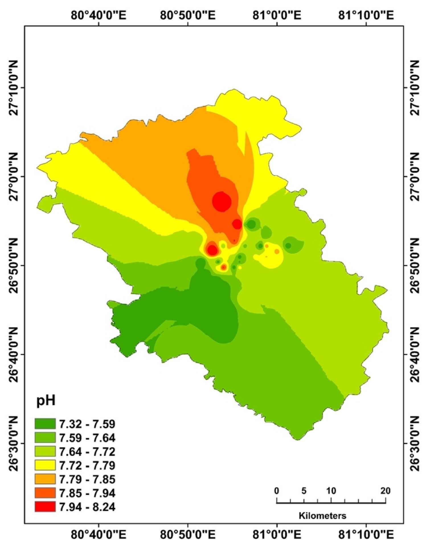
3.1.1. Hydrogen Ion Concentration (pH)

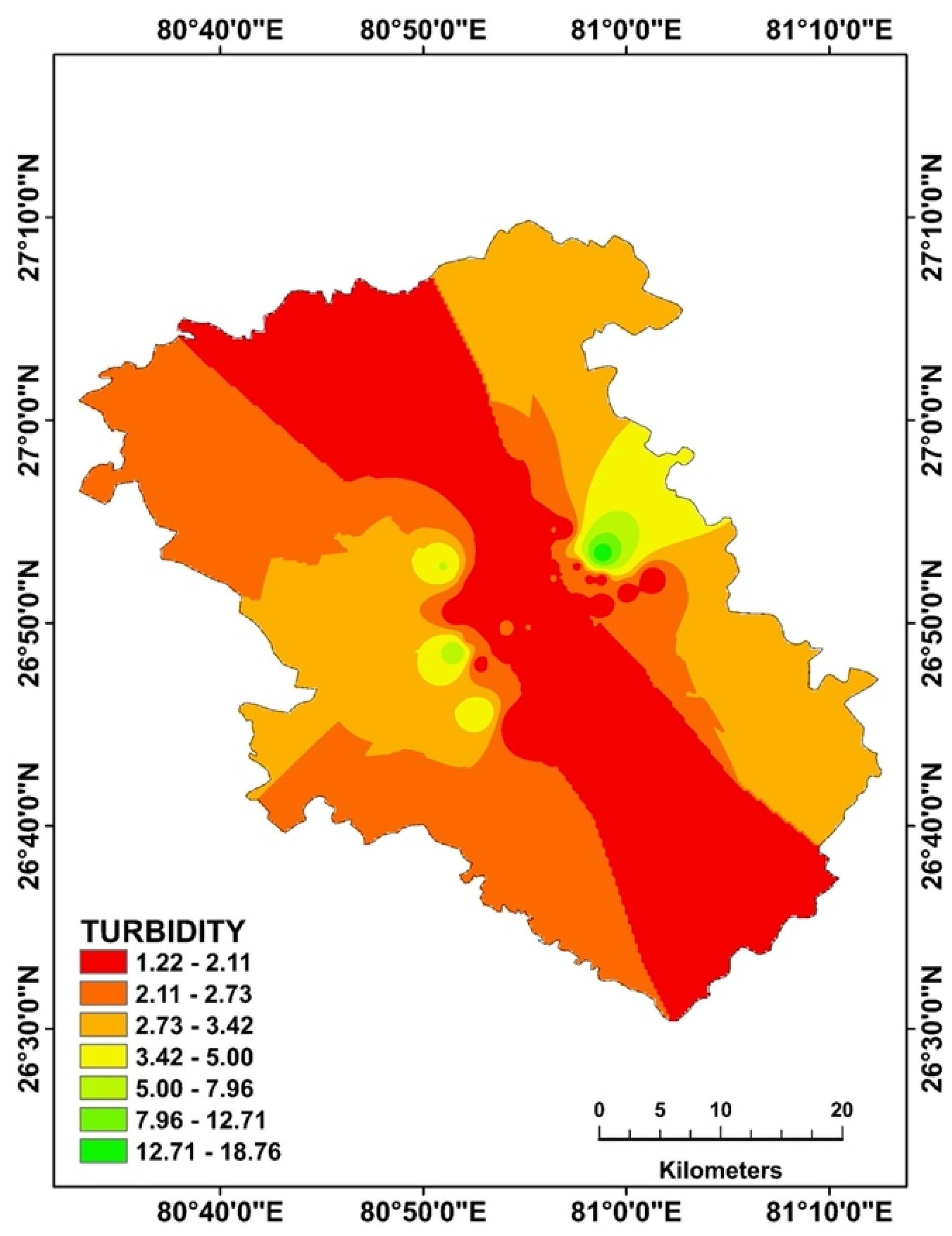
The pH varied between 7.32 (minimum) to 8.25 (maximum) in this study in Figure 3, which is within the acceptable range and indicates the alkalinity of groundwater (the ideal pH range for drinking purposes is 6.5–8.5).

3.1.2. Turbidity

The relative clarity of any liquid is measured by turbidity. It measures the proportion of light dispersed by substances in the water when the water sample is illuminated. Excessive turbidity in water is not pleasing and can be a health hazard. If the causes of high turbidity are not addressed, the regrowth of waterborne pathogens can be accelerated, leading to waterborne diseases [55]. The permissible limits for turbidity are 1 to 5 NTU, respectively, as per IS:10500-2012. In the current study, turbidity varied between 1.2 to 19.04 NTU, which exceeds the permissible range, as shown in Figure 4.

3.1.3. Total Dissolved Solids (TDS)

In this study, TDS varied from 300 to 1090${\mathrm{m}\mathrm{g}\mathrm{L}}^{-1}$ (TDS for safe water by BIS is <500 ${\mathrm{m}\mathrm{g}\mathrm{L}}^{-1}$). The primary sources of TDS are cultivation practices, leaching of soil, urban runoff, and sources of point pollution that discharge through industry or sewage treatment plants [53,56].

3.1.4. Chloride (${\mathrm{C}\mathrm{l}}^{-}$)

Chloride concentration ranged from 14.68 to 112 ${\mathrm{m}\mathrm{g}\mathrm{L}}^{-1}$, within the permissible range (250 ${\mathrm{m}\mathrm{g}\mathrm{L}}^{-1}$). High chloride content in groundwater is harmful to the health of human beings [57].

3.1.5. Total Alkalinity

The acceptable range for alkalinity in drinking water is up to 200 ${\mathrm{m}\mathrm{g}\mathrm{L}}^{-1}$, above which water tastes bitter [58]. Alkalinity ranged from 170 to 490 ${\mathrm{m}\mathrm{g}\mathrm{L}}^{-1}$ in this study, which is within acceptable limits (600 ${\mathrm{m}\mathrm{g}\mathrm{L}}^{-1}$).

3.1.6. Total Hardness

In this study, the hardness in water ranged from 190 to 495 ${\mathrm{m}\mathrm{g}\mathrm{L}}^{-1}$, which is within the acceptable range (600 ${\mathrm{m}\mathrm{g}\mathrm{L}}^{-1}$). Heart diseases and kidney stones can be caused due to high concentrations of hardness in groundwater [59].

3.1.7. Sulphate (${\mathrm{S}\mathrm{O}}_4^{2-}$)

Sulphate concentration varied from 2 to 160 ${\mathrm{m}\mathrm{g}\mathrm{L}}^{-1}$ in the current work, within the acceptable range of 200 ${\mathrm{m}\mathrm{g}\mathrm{L}}^{-1}$ [60].

3.1.8. Nitrate (${\mathrm{N}\mathrm{O}}_3^{-}$)

Nitrate is a naturally existing ion and is an integral part of the nitrogen cycle. However, nitrate in groundwater is troublesome because it can cause Methemoglobinemia in children under six months [60,61,62]. Generally, high nitrogen concentration beyond the permissible range of 45 ${\mathrm{m}\mathrm{g}\mathrm{L}}^{-1}$ [57] poses a health hazard [63]. In the present study, nitrate concentrations range from 0.43 to 100 ${\mathrm{m}\mathrm{g}\mathrm{L}}^{-1}$, exceeding the permissible range. High nitrate concentrations in drinking water increase health risks in pregnant women and newborns [64].

3.1.9. Fluoride (${\mathrm{F}}^{-}$)

Fluoride is a common constituent of groundwater. Natural sources are connected to various types of rocks and volcanic activity. Agricultural (use of phosphatic fertilizers) and industrial (clays used in ceramic industries or burning of coals) activities also contribute to high fluoride concentrations in groundwater [65]. It is among the lightest halogens and the most reactive elements [66]. It is usually found as a trace quantity or a significant ion in high concentration [67]. Fluoride is present in groundwater mainly through the interaction of fluoride-bearing minerals and host rocks with groundwater. This study’s fluoride concentration varied from 0.15 to 1.15 ${\mathrm{m}\mathrm{g}\mathrm{L}}^{-1}$, within the acceptable limit (1–1.5 ${\mathrm{m}\mathrm{g}\mathrm{L}}^{-1}$).

3.1.10. Iron (Fe)

The most frequent source of iron in groundwater is the weathering of iron-containing mineral rocks. Iron exists naturally in the aquifers in the ${\mathrm{F}\mathrm{e}}^{2+}$ state, but the concentration of iron rises after its dissolution in groundwater. It is soluble in this form and does not typically cause any health hazard, but when the ${\mathrm{F}\mathrm{e}}^{2+}$ state is oxidized to the ${\mathrm{F}\mathrm{e}}^{3+}$ state, insoluble hydroxides are formed in groundwater due to its contact with atmospheric oxygen [68]. Therefore, compared with surface water, there are higher iron concentrations in the groundwater. The iron content varied from 0.01 to 0.5 ${\mathrm{m}\mathrm{g}\mathrm{L}}^{-1}$, within the acceptable range of 1.0 ${\mathrm{m}\mathrm{g}\mathrm{L}}^{-1}$ [60,61,62].

3.1.11. Arsenic (As)

Arsenic content in the studied area’s water fluctuated between 0.0002 to 0.017 ${\mathrm{m}\mathrm{g}\mathrm{L}}^{-1}$, within the permissible limit of 0.01 to 0.05 ${\mathrm{m}\mathrm{g}\mathrm{L}}^{-1}$. Arsenic concentration can be significantly elevated in groundwater with sulfide mineral deposits and volcanic rock deposits. Arsenic also enters the atmosphere through natural biomethylation and reduces to arsine at low temperatures. Long-term ingestion of arsenic-contaminated water can cause skin lesions, hard patches on the palms and soles of the feet (hyperkeratosis), diabetes, pulmonary disease, and cardiovascular disease [2].

3.1.12. Magnesium (${\mathrm{M}\mathrm{g}}^{2+}$)

Magnesium concentration is a significant parameter that affects the hardness of water. Magnesium concentration varied between 17.9 to 122.79 ${\mathrm{m}\mathrm{g}\mathrm{L}}^{-1}$, more than the acceptable range (100 ${\mathrm{m}\mathrm{g}\mathrm{L}}^{-1}$).

3.1.13. Calcium (${\mathrm{C}\mathrm{a}}^{2+}$)

Calcium is introduced into the aquifer system through the leaching of calcium-containing minerals. Calcium concentration varied from 8.1 to 75 ${\mathrm{m}\mathrm{g}\mathrm{L}}^{-1}$, within the permissible limits (200 ${\mathrm{m}\mathrm{g}\mathrm{L}}^{-1}$).

3.2. Water Quality Index (WQI)

This study utilized all thirteen parameters to calculate the WQI. The WQI was determined based on drinking water quality standards set by the Indian Council for Medical Research [63], the Bureau of Standards of India (BIS), and the World Health Organization [55]. The weighted arithmetic index method [64] was employed to calculate the WQI for water, involving the following successive steps.

3.2.1. Weightage Factor ${(\mathrm{W}}_{\mathrm{i}}$)

The parameters’ weights ${(\mathrm{w}}_{\mathrm{i}}$) were allocated based on their importance in ensuring water quality. The weightage factor was determined in the following manner.

$${\mathrm{W}}_{\mathrm{i}}={\mathrm{w}}_{\mathrm{i}}/{\sum }_{i=1}^{n}wi$$

where ${\mathrm{W}}_{\mathrm{i}}$ indicates relative weight, ${\mathrm{w}}_{\mathrm{i}}$indicates the weight of every parameter, and n indicates the number of parameters.

3.2.2. Calculation of Sub-Index (${\mathrm{Q}}_{\mathrm{i}}$)/Quality Rating

The calculation of the sub-index is as follows:

$$(\mathrm{S}\mathrm{u}\mathrm{b}-\mathrm{i}\mathrm{n}\mathrm{d}\mathrm{e}\mathrm{x}){\mathrm{Q}}_{\mathrm{i}}=({\mathrm{V}}_{\mathrm{e}}-{\mathrm{V}}_{\mathrm{i}})/({\mathrm{V}}_{\mathrm{s}}-{\mathrm{V}}_{\mathrm{i}})\times 100$$

where ${\mathrm{V}}_{\mathrm{e}}$ indicates an estimated value for the ith parameter, ${\mathrm{V}}_{\mathrm{i}}$ indicates an ideal value for the ith parameter, ${\mathrm{V}}_{\mathrm{s}}$ indicates a standard permissible value for the ith parameter, and ${\mathrm{Q}}_{\mathrm{i}}$ indicates the quality rating for the ith water quality parameter.

3.2.3. Calculation of WQI

To calculate WQI, first there is a calculation of the sub-index for every parameter with the use of the following formula:

$${{\mathrm{S}\mathrm{I}}_{\mathrm{i}}={\mathrm{w}}_{\mathrm{i}}\times \mathrm{q}}_{\mathrm{i}}$$

where ${\mathrm{S}\mathrm{I}}_{\mathrm{i}}$ indicates the sub-index of its parameter, qi indicates the sub-rating based on the concentration of ith, and n represents the numbers of the parameter.

Each value of the sub-index of each groundwater sample was added to calculate the overall WQI [34,66,67].

$$\mathrm{W}\mathrm{Q}\mathrm{I}=\sum {\mathrm{S}\mathrm{I}}_{\mathrm{i}}$$

Calculated values of WQI were classified into five different categories: very good, good, poor, very poor, and unfit for drinking, as depicted in

Table 4. Groundwater quality as per WQI range.

WQI	Category
0–34	Very good
35–44	Good
45–54	Moderate
55–64	Poor
>65	Unfit for drinking

.

4. Result

4.1. Correlations Matrix and Statistical Assessment

Groundwater quality parameters were assessed for the tabulation of the correlation matrix and general statistical analysis, as given in Table 2 and Table 3. A correlation matrix of thirteen different parameters was created with the help of MS Excel 2017. Among the thirteen parameters, pH positively correlates with turbidity, chloride, sulphate, and calcium. Turbidity is significantly correlated with chloride, fluoride, and arsenic. Chloride has a positive correlation with sulphate, fluoride, and calcium. Sulphate positively correlates with arsenic and calcium, and alkalinity negatively correlates with hardness, fluoride, and arsenic. Fluoride is negatively correlated with arsenic.

Among the maximum quality parameters, there is a positive correlation with each other. Higher concentrations of Fe and As can trigger the presence of other heavy metals such as Pb, Cd, and Cr. As they are much more critical and crucial heavy metals, they require careful monitoring for the future groundwater quality of the region. The presence of Fe, (${\mathrm{S}\mathrm{O}}_4^{2-}$), and $\left({\mathrm{N}\mathrm{O}}_3^{-}\right)$can lead to the existence of cadmium [69].

4.2. Spatial Distribution Pattern

The spatial distribution pattern was generated from groundwater quality parameters, as depicted in Figure 3, Figure 4, Figure 5, Figure 6, Figure 7, Figure 8, Figure 9, Figure 10, Figure 11, Figure 12, Figure 13, Figure 14 and Figure 15. The spatial distribution map of pH shows that the north-central part has alkaline water, as illustrated in Figure 3. Therefore, an alkali pH is more advantageous for forming fluoride solutions [70,71,72]. Turbidity exceeds the permissible range in the east-central part, making it unfit for drinking. The alkalinity is most significant in the central patches and eventually decreases outward, as shown in Figure 7. It is clear from the spatial distribution pattern of total hardness that there is moderately hard groundwater in the study area, especially in the central region. Sulphate lies inside the acceptable range in the region and is a crucial quality parameter. The spatial distribution map of chloride reveals that the distribution of chloride is low in the area (Figure 6). Fluoride distribution is highest in the north-central part of the region. Its concentration is within the acceptable range (Figure 10). Several factors contribute to fluoride concentration in groundwater; in particular pH, temperature, absence or presence of complexed or precipitated colloids and ions, the solubility of fluoride-containing minerals (apatite and biotite), the aquifer anion exchange capacity, the size and type of formations that the groundwater passes through, and the time of contact that the water persists in association with these formations are the leading causes of formation of fluoride in groundwater [73]. The extensive use of nitrogen fertilizers like urea, ammonium nitrate, ammonium sulphate, dry ammonium phosphate, NPK, and NP complex [74] have led to an increase in nitrate levels in both surface water and groundwater over the past five decades. Since soils do not absorb nitrates, they are leached into surface water bodies and groundwater. Elevated nitrate levels in drinking water can result in a severe blood disorder known as ‘blue baby syndrome’ or Methemoglobinemia, particularly affecting infants under six months old. Moreover, there is a potential link between excessive nitrate consumption and the synthesis of carcinogenic nitrosamines in the human body [75]. The nitrate concentration exceeds the acceptable range in the central region, which may affect human health (Figure 10). Further, ammonification of animal waste and plant and animal remains in soil produces ammonia that endures nitrification. Unlined septic tanks and unplanned sewage systems may cause high nitrate concentrations in the region, contaminating the phreatic aquifers [76,77,78]. There is a requirement for regular monitoring to evaluate the effects of nitrate on the health of humans. The concentration of heavy metals does not have any notable existence in the region (Figure 12 and Figure 13). The study shows that there is varying concentration of iron throughout the study area, but its concentration is within the acceptable limit. Once (${\mathrm{F}\mathrm{e}}^{2+}$) is converted into the (${\mathrm{F}\mathrm{e}}^{3+}$) state, it becomes harmful and causes health hazards. This situation can be avoided by increasing groundwater levels in the affected areas through groundwater recharge (Figure 12). The concentration of arsenic falls within the permissible range, as indicated in Figure 13. The study area displays fluctuating but acceptable calcium concentration levels, as depicted in Figure 15. Additionally, the magnesium concentration in the north-central region slightly surpasses the permissible range (Figure 14).

4.3. Water Quality Index

Using Arc-GIS 10.8, WQI maps were created based on selected quality parameters illustrating various quality classes at each hydro station, including very good, good, moderate, poor, and unsuitable for drinking (Table 4 and

Table 5. Water quality index and its category for all hydro stations of the study area.

Hydro-Station	Sample Code	Source of Sample	Value of WQI	Category
Kadam Rasool	T1	Tube well	10.39	Very good
Triveni Nagar	T2	Tube well	10.51	Very good
Madiyawa	T3	Tube well	39.21	Good
Faizullahganj	T4	Tube well	10.35	Very good
Motijheel	T5	Tube well	10.34	Very good
Rajajipuram	T6	Tube well	13.16	Very good
Balaganj	T7	Tube well	10.44	Very good
Mawaiya	T8	Tube well	10.52	Very good
Daliganj	T9	Tube well	10.24	Very good
Aishbagh	H1	Hand pump	11.85	Very good
High Court	H2	Hand pump	8.89	Very good
Dubagga	H3	Hand pump	5.05	Very good
Hanskhera	H4	Hand pump	6.86	Very good
Sikandarpur	H5	Hand pump	5.72	Very good
Amausi Airport	H6	Hand pump	6.68	Very good
Pariwartan Chowk	W1	Borehole	5.53	Very good
Alamnagar	W2	Borehole	7.50	Very good
South City	W3	Borehole	5.79	Very good
KMCL University	W4	Borehole	7.37	Very good
Husainabad	W5	Borehole	8.45	Very good
HAL	W6	Borehole	6.67	Very good
Polytechnic	W7	Borehole	7.36	Very good
Sikandarbagh	W8	Borehole	3.63	Very good
Lalkuan	W9	Borehole	7.50	Very good
Devpur Para	W10	Borehole	10.73	Very good
Alambagh	W11	Borehole	7.73	Very good
Khurram Nagar	W12	Borehole	8.31	Very good
Kukrail	W13	Borehole	168.68	Unfit for drinking
Naka	W14	Borehole	6.62	Very good
Nishatganj	W15	Borehole	8.49	Very good
Indira Nagar	W16	Borehole	7.83	Very good
Naharia	W17	Borehole	10.34	Very good
Lalbagh	W18	Borehole	6.81	Very good
Jankipuram	W19	Borehole	21.38	Very good
Charbagh	W20	Borehole	10.34	Very good
Vrindawan	W21	Borehole	10.89	Very good
Chinhat	W22	Borehole	2.64	Very good
1090 Chauraha	W23	Borehole	11.13	Very good
RSAC	W24	Borehole	10.46	Very good
Manak Nagar	W25	Borehole	10.57	Very good

, Figure 16). The WQI map reveals that 86% of the area exhibits very good groundwater quality, 14.63% falls under the good to moderate quality range (35–45), and only 0.37% is considered unsuitable for drinking (Figure 16). Overall, the groundwater quality in most of the study region is very good, making it suitable for drinking and irrigation (Figure 17 and Figure 18).

5. Discussion

The pH level of water gauges its acid–base balance. Water can be either alkaline, neutral, or acidic based on its pH value. Water with extremely high or low pH levels is unsafe to drink and unsuitable for specific uses. The World Health Organization (WHO) suggests maintaining a pH between 6.5 and 8.5 [61]. Water with a pH above 10 can irritate the eyes, skin, and mucous membranes if used by people [79]. It can also cause hair fibers to swell and potentially result in gastrointestinal irritation. Conversely, using water with a low pH produces similar effects and affects disinfection efficiency [80]. Verma et al. (2021) recorded a maximum pH of 8.6 in the Lucknow district. In the current study, pH levels ranged from 7.32 to 8.25 [81].

Turbidity indicates the cloudiness of water resulting from particles held in suspension, like clay, silts, chemical precipitates (such as manganese and iron), and organic matter (including plant remnants and organisms). Heightened turbidity diminishes water clarity due to the scattering and absorption of transmitted light. There have been instances where elevated turbidity has been linked to disease outbreaks [82]. However, a direct correlation between eliminating turbidity and reducing pathogens has not been proven [83]. Similarly, efforts to establish connections between the turbidity levels of drinking water and rates of local gastrointestinal diseases have yielded mixed outcomes. Some studies suggest a link, while others do not [82,84]. Thus, although correlations might exist in specific water supplies, a consistent relationship remains unestablished. In Gautam Buddh Nagar, U.P., Banerjee et al. (2021) documented a maximum turbidity of 56 NTU [85]. In the current study, turbidity ranged from 1.2 to 19.04 NTU, surpassing the permissible range.

Total Dissolved Solids (TDS) encompasses all dissolved mineral components and other solids in water. TDS is an indicator of water’s suitability for diverse applications. Water with TDS levels below 500 ${\mathrm{m}\mathrm{g}\mathrm{L}}^{-1}$ is considered suitable for drinking [60]. Elevated TDS values can impact water’s taste, hardness, and corrosive tendencies [86]. If TDS concentration surpasses 1000 ${\mathrm{m}\mathrm{g}\mathrm{L}}^{-1}$, the water becomes unpalatable for consumption [60]. In the Lucknow district, Verma et al. (2021) identified a peak TDS level of 805.3 ${\mathrm{m}\mathrm{g}\mathrm{L}}^{-1}$ [81]. In the present study, TDS varied between 300 and 1090 ${\mathrm{m}\mathrm{g}\mathrm{L}}^{-1}$, exceeding the permissible range.

Chlorides represent significant inorganic anions found in natural water sources. Chloride can stem from natural origins or accumulate in groundwater through weathering, sedimentary rock and soil leaching, agricultural practices, and domestic wastewater. Elevated chloride levels indicate pollution from organic waste from industrial or animal sources [87]. Nevertheless, a rise in ${\mathrm{C}\mathrm{l}}^{-}$ concentration can result in detrimental effects such as heart and kidney impairments, digestive issues, and alterations in taste and palatability [88]. In Lucknow City, Singh et al. (2020) documented the highest chloride reading at 122 ${\mathrm{m}\mathrm{g}\mathrm{L}}^{-1}$ [89]. Chloride levels within this study varied from 14.68 to 112 ${\mathrm{m}\mathrm{g}\mathrm{L}}^{-1}$, remaining within the permissible range (250 ${\mathrm{m}\mathrm{g}\mathrm{L}}^{-1}$).

Alkalinity, also known as buffering capacity, signifies a water’s ability to neutralize acid. Slightly elevated alkaline water might benefit individuals with high cholesterol, diabetes, and hypertension. Additionally, it supports the immune system and carries advantages like weight management and potential cancer resistance. However, prolonged consumption of highly alkaline water could lead to adverse effects, including skin irritation, nausea, vomiting, hand tremors, and muscle spasms, particularly around the facial extremities. It might also result in a reduction of free calcium levels within the human body [90]. In the Lucknow region, Kumar et al. (2016) observed the highest alkalinity recorded at 450 ${\mathrm{m}\mathrm{g}\mathrm{L}}^{-1}$ [91]. Alkalinity within this study ranged from 170 to 490 ${\mathrm{m}\mathrm{g}\mathrm{L}}^{-1}$, remaining well within the acceptable limits (600 ${\mathrm{m}\mathrm{g}\mathrm{L}}^{-1}$).

Elevated hardness levels can impact various aspects, including water supply systems, excessive soap usage, and the potential for arterial calcification. These effects might contribute to urinary concretions, kidney and bladder diseases, and gastrointestinal disorders [88]. In his discussion, Sengupta explored a converse connection between water hardness and cardiovascular ailments [92]. Kozisek’s findings indicate that hardness concentrations exceeding allowable limits increase the risk of conditions like gallstones, urinary stones, kidney stones, and arthropathies within the population [93]. In Lucknow city, Singh et al. (2020) documented the highest recorded hardness at 419 ${\mathrm{m}\mathrm{g}\mathrm{L}}^{-1}$ [89]. The present study recorded water hardness varied from 190 to 495 ${\mathrm{m}\mathrm{g}\mathrm{L}}^{-1}$, all within the permissible range (600 ${\mathrm{m}\mathrm{g}\mathrm{L}}^{-1}$) [60].

While not inherently toxic, sulphate can produce undesirable effects when consumed in excessive quantities. Elevated sulphate levels can induce catharsis, dehydration, and diarrhea, occasionally altering methemoglobin and sulfhemoglobin levels within the human body system [93,94]. High sulphate levels can also change water’s taste, rendering it bitter, particularly if concentrations surpass 250 ${\mathrm{m}\mathrm{g}\mathrm{L}}^{-1}$. Sulphate might trigger a laxative effect, potentially leading to dehydration and heightened risk, especially for infants. Once sulphate levels exceed 400 ${\mathrm{m}\mathrm{g}\mathrm{L}}^{-1}$, the water becomes unsuitable for infant use (including drinking and food preparation). In the Lucknow area, Singh et al. (2020) identified the highest sulphate concentration recorded at 86.4 ${\mathrm{m}\mathrm{g}\mathrm{L}}^{-1}$ [89]. The current study observed sulphate levels ranging from 2 to 160 ${\mathrm{m}\mathrm{g}\mathrm{L}}^{-1}$, all within the permissible range of 200 ${\mathrm{m}\mathrm{g}\mathrm{L}}^{-1}$.

Nitrate is a naturally occurring ion linked to the nitrogen cycle [95]. Exceeding acceptable nitrate levels can lead to “blue baby syndrome” and thyroid disorders [96]. Nitrate groundwater contamination is a global issue, often associated with agricultural activities. In India, 11 out of 28 states have nitrate concentrations exceeding the acceptable level of 45 ${\mathrm{m}\mathrm{g}\mathrm{L}}^{-1}$ [75]. Rajasthan, for instance, has 22% of villages with excessive nitrate contamination [97]. As per Indian standards, the permissible nitrate level in potable water is 45 ${\mathrm{m}\mathrm{g}\mathrm{L}}^{-1}$. Verma et al. (2021) reported a maximum nitrate level of 108 ${\mathrm{m}\mathrm{g}\mathrm{L}}^{-1}$in Lucknow [81]. In the present study, nitrate concentrations range from 0.43 to 100 ${\mathrm{m}\mathrm{g}\mathrm{L}}^{-1}$, exceeding the permissible range.

Fluoride is frequently present in minerals and can be leached out due to erosion by rainwater, resulting in the pollution of ground and surface waters [98]. Multiple countries and states, including India, China, Japan, Sri Lanka, Iran, Pakistan, Turkey, Southern Algeria, Mexico, Korea, Ohio, Wisconsin, South Carolina, Kenya, Ghana, Norway, Canada, Ethiopia, North Jordan, Malawi, Brazil, and Italy, have been identified with excessive fluoride levels in their groundwater [3]. In Uttar Pradesh’s Sonbhadra district, Prof. H.K. Pandey and co-authors studied fluoride contamination and the groundwater release mechanism in hard rock aquifers. India is particularly affected, with an estimated 62 million people experiencing dental, skeletal, and nonskeletal fluorosis [4]. Verma et al. (2021) reported a maximum fluoride level of 0.9 ${\mathrm{m}\mathrm{g}\mathrm{L}}^{-1 }$in the Lucknow area [81]. The fluoride concentration in the present study ranged from 0.15 to 1.15 ${\mathrm{m}\mathrm{g}\mathrm{L}}^{-1}$, which falls within the acceptable range of (1–1.5 ${\mathrm{m}\mathrm{g}\mathrm{L}}^{-1}$).

The body requires iron to synthesize oxygen-transport proteins, particularly hemoglobin and myoglobin. Imbalances in iron levels, whether deficient or excessive, can adversely affect both plants and animals [99]. Elevated iron levels in natural water sources pose potential risks to human health and the environment. While iron overload is less frequent than its deficiency, it can result in severe health problems such as heart and liver issues, diabetes, cancer, and even neurodegenerative disorders [100,101,102,103]. Iron contamination in groundwater has become a significant concern in multiple countries, including India, Sweden, Canada, the USA, Brazil, South Africa, Kazakhstan, Iran, Russia, China, New Zealand, Australia, and Bangladesh [2,104]. In India, Rajasthan, Orissa, and Tripura are particularly affected, with iron levels varying from 0.01 to 0.5 ${\mathrm{m}\mathrm{g}\mathrm{L}}^{-1}$, within the acceptable range of 1.0 ${\mathrm{m}\mathrm{g}\mathrm{L}}^{-1}$ [75]. Kumar et al. (2016) documented the highest iron level of 1.38 ${\mathrm{m}\mathrm{g}\mathrm{L}}^{-1}$in Lucknow [91]. In the present study, iron concentrations ranged from 0.01 to 0.5 ${\mathrm{m}\mathrm{g}\mathrm{L}}^{-1}$, which falls within the acceptable range of 1.0 ${\mathrm{m}\mathrm{g}\mathrm{L}}^{-1}$.

Arsenic has been classified as a class I human carcinogen by the International Agency of Research on Cancer (IARC) [105]. Prolonged oral exposure to inorganic arsenic leads to neurological and hematological toxicity in humans [106]. Excessive exposure to arsenic heightens the risk of ailments such as lung, kidney, and skin cancer [107]. Arsenic contamination in groundwater is prevalent in Bangladesh, India (West Bengal), China, Russia, Brazil, the USA, and Australia. In India, nitrate contamination in groundwater has been reported with levels above 100 ${\mathrm{m}\mathrm{g}\mathrm{L}}^{-1}$, and other countries like Iran, Mexico, China, South Africa, and Argentina have documented levels above 50–100 ${\mathrm{m}\mathrm{g}\mathrm{L}}^{-1}$ [4]. The problem of arsenic contamination is widespread in India, impacting around 40 million people residing in at-risk areas [2]. Singh et al. (2020) identified the highest arsenic concentration of 0.04 ${\mathrm{m}\mathrm{g}\mathrm{L}}^{-1}$ in the Lucknow area [89]. The arsenic content in the study area fluctuated between 0.0002 to 0.017 ${\mathrm{m}\mathrm{g}\mathrm{L}}^{-1}$, within the acceptable range of 0.01 to 0.05 ${\mathrm{m}\mathrm{g}\mathrm{L}}^{-1}$.

Magnesium is vital in bone mineralization, muscle relaxation, and cellular functions [108]. Inadequate magnesium intake has been connected to conditions like high blood pressure, the accumulation of arterial plaque, soft tissue calcification, elevated cholesterol, and arterial stiffening [109]. High magnesium levels in drinking water have been linked to hypertension and cardiovascular issues, which can potentially be life-threatening [110]. Verma et al. (2021) recorded the highest magnesium concentration in the Lucknow region at 65 ${\mathrm{m}\mathrm{g}\mathrm{L}}^{-1}$ [81]. In the current study, magnesium concentrations ranged from 17.9 to 122.79 ${\mathrm{m}\mathrm{g}\mathrm{L}}^{-1}$, exceeding the permissible range of 100 ${\mathrm{m}\mathrm{g}\mathrm{L}}^{-1}$.

Excessive calcium intake can lead to notable adverse effects such as hypercalcemia, elevated urinary calcium levels, formation of urinary tract stones, soft tissue calcification (particularly in the kidneys and arterial walls), and suppression of natural bone remodeling [111]. In the Lucknow region, Singh et al. (2020) noted the highest calcium level of 101 ${\mathrm{m}\mathrm{g}\mathrm{L}}^{-1}$ [89]. This study revealed calcium concentrations spanning 8.1 to 75 ${\mathrm{m}\mathrm{g}\mathrm{L}}^{-1}$, all within the allowable limits (200 ${\mathrm{m}\mathrm{g}\mathrm{L}}^{-1}$).

6. Conclusions

The conclusion of the current research in the flat alluvial region of central India reveals that groundwater quality is overall excellent in the area. The thick Quaternary sediments form a multi-layered aquifer system, considered one of the best from a hydrogeological perspective. This setup allows for a good flux of water, which enhances the groundwater quality. However, unsustainable human activities, such as the use of synthetic nitrogen fertilizers, combustion engines in vehicles, municipal effluent disposal through sludge spreading on fields, atmospheric emissions from energy production, septic tanks, leaking slurry or manure tanks, leaking sewage systems, accidental spills of nitrogen-rich compounds, and nitrogen-rich waste disposal using sound injection techniques, are observed in various locations and have increased groundwater nitrate concentrations, especially in the north-central parts of the study area. Urban areas with high population densities experience considerable water resource quality impacts, primarily due to intensified human activity, industrialization, and agricultural practices. These factors synergistically contribute to elevated levels of nitrates and magnesium in water content. Agricultural runoff from nitrogen-rich fertilizers and untreated urban wastewater discharge introduce substantial nitrate concentrations. Urbanization and land use changes result in decreased infiltration, leading to increased surface runoff that carries nitrates into water bodies. Human activities, vehicular emissions, industrial discharges, and improper waste disposal practices also escalate nitrate and magnesium pollution. Consequently, the elevated levels of nitrates and magnesium in water content underscore the pressing need for comprehensive strategies to manage pollution and sustain urban water resources. High turbidity has been observed in the Kukrail region, while magnesium levels have surpassed the permissible level in some areas. The remaining areas have potable and safe groundwater, as indicated by their lower WQI values, ensuring secure water quality for drinking and domestic purposes. The conclusion from the analysis in this study, based on WQI, is that the groundwater in the area is safe and suitable for drinking.

7. Recommendations

• Regular Monitoring: Establishing an ongoing groundwater quality monitoring system is imperative for promptly identifying changes or potential sources of contamination that may emerge over time.
• Focused Investigation: A comprehensive investigation is advised to pinpoint the precise origins of contamination in the area. This in-depth analysis will facilitate the development of targeted solutions.
• Treatment Implementation: Immediate measures should be taken to apply suitable treatment techniques in the Kukrail region to bring the water quality up to acceptable standards.
• Public Awareness: Public awareness campaigns will empower residents with knowledge about their groundwater quality. Information about the overall water quality, the areas with unfit water, and potential health risks can help residents make informed decisions about water use.
• Localized Solutions: Since most of the area falls under very good water quality categories, it is essential to focus on localized solutions to address emerging water quality issues. This might involve promoting best practices for agricultural and industrial activities that could impact groundwater quality.
• Collaboration with Authorities: Close collaboration with local authorities and environmental agencies is pivotal in influencing policy formulation and regulations concerning groundwater management.
• Regular Updates: Keep the public and local authorities informed about the progress of groundwater quality improvements. Regular updates and transparent communication can build trust and foster cooperation in managing this valuable resource.

References

1. Ouyang, T.; Zhu, Z.; Kuang, Y. Assessing impact of urbanization on river water quality in the Pearl River Delta Economic Zone, China. Environ. Monit. Assess. 2006, 120, 313–325. [Google Scholar]
2. Saha, D.; Sahu, S. A decade of investigations on groundwater arsenic contamination in Middle Ganga Plain, India. Environ. Geochem. Health 2015, 38, 315–337. [Google Scholar]
3. Brindha, K.; Elango, L.; RNV, N. Spatial and temporal variation of uranium in a shallow weathered rock aquifer in southern India. J. Earth Syst. Sci. 2011, 120, 911–920. [Google Scholar]
4. Meraj, G. Assessing the Impacts of Climate Change on Ecosystem Service Provisioning in Kashmir Valley India. Ph.D. Thesis, Suresh Gyan Vihar University, Jaipur, India, 2021. [Google Scholar]
5. Alban, K. Simulink application on dynamic modeling of biological waste water treatment for aerator tank case. Int. J. Sci. Technol. Res. 2014, 3, 69–72. [Google Scholar]
6. Alban, K.; Irma, K.; Elisabeta, P. Simulink programming for dynamic modelling of activated sludge process: Aerator and settler tank case. Fresenius Environ. Bull. 2016, 25, 2891–2899. [Google Scholar]
7. Mangukiya, R.; Bhattacharya, T.; Chakraborty, S. Quality characterization of groundwater using water quality index in Surat city, Gujarat, India. Int. Res. J. Environ. Sci. 2012, 1, 4–23. [Google Scholar]
8. Kavitha, M.T.; Divahar, R.; Meenambal, T.; Shankar, K.; Vijay Singh, R.; Haile, T.D.; Gadafa, C. Dataset on the assessment of water quality of surface water in Kalingarayan Canal for heavy metal pollution, Tamil Nadu. Data Brief 2019, 22, 878–884. [Google Scholar]
9. Kavitha, M.T.; Shankar, K.; Divahar, R.; Meenambal, T.; Saravanan, R. Impact of industrial wastewater disposal on surface water bodies in Kalingarayan canal, Erode district, Tamil Nadu, India. Arch. Agric. Environ. Sci. 2019, 4, 379–387. [Google Scholar]
10. Sinha, K.K.; Gupta, M.K.; Banerjee, M.K.; Meraj, G.; Singh, S.K.; Kanga, S.; Farooq, M.; Kumar, P.; Sahu, N. Neural Network-Based Modeling of Water Quality in Jodhpur, India. Hydrology 2022, 9, 92. [Google Scholar]
11. Panigrahi, T.; Das, K.K.; Dey, B.S.; Panda, R.B. Assessment of Water Quality of river Sono, Balasore. Int. J. Environ. Sci. 2012, 3, 49–56. [Google Scholar]
12. Gebrehiwot, A.B.; Tadesse, N.; Jigar, E. Application of water quality index to assess suitability of groundwater quality for drinking purposes in Hantebet watershed, Tigray, Northern Ethiopia. ISABB J. Food Agric. Sci. 2011, 1, 22–30. [Google Scholar]
13. WHO. Guideline for Drinking Water Quality, 4th ed.; World Health Organization: Geneva, Switzerland, 2017. [Google Scholar]
14. Diersing, N.; Nancy, F. Water Quality: Frequently Asked Questions; Florida Brooks National Marine Sanctuary: Key West, FL, USA, 2009. [Google Scholar]
15. Panneerselvam, B.; Paramasivam, S.K.; Karuppannan, S.; Selvaraj, P. A GIS-based evaluation of hydro chemical characterization of groundwater in hard rock region, South Tamil Nadu. India Arab. J. Geosci. 2020, 13, 837. [Google Scholar] [CrossRef]
16. Smith, D.G. A better water quality indexing system for rivers and streams. Water Res. 1990, 24, 1237–1244. [Google Scholar] [CrossRef]
17. Debnath, J.; Sahariah, D.; Saikia, A.; Meraj, G.; Nath, N.; Lahon, D.; Annayat, W.; Kumar, P.; Chand, K.; Singh, S.K.; et al. Shifting Sands: Assessing Bankline Shift Using an Automated Approach in the Jia Bharali River, India. Land 2023, 12, 703. [Google Scholar] [CrossRef]
18. Stambuk Giljanvoic, N. Water quality evaluation by index in Dalmatia. Water Res. 1999, 33, 3423–3440. [Google Scholar] [CrossRef]
19. Pesce, S.F.; Wunderlin, D.A. Use of water quality indices to verify the impact of Cordoba city (Argentina) on Suquiariver. Water Res. 2000, 34, 2915–2936. [Google Scholar] [CrossRef]
20. Sargaonkar, A.; Deshpande, V. Development of an overall index of pollution for surface water based on general classification scheme in Indian context. Environ. Monit. Assess. 2003, 89, 43–67. [Google Scholar] [CrossRef]
21. Saeedi, M.; Abessi, O.; Sharifi, F.; Meraji, H. Development of Ground Water Quality Index. Environ. Monit. Assess. 2010, 163, 327–335. [Google Scholar] [CrossRef]
22. Alexakis, D.E. Meta-Evaluation of Water Quality Indices. Application into Groundwater Resources. Water 2020, 12, 1890. [Google Scholar] [CrossRef]
23. Yisa, J.; Jimoh, T. Analytical Studies on Water Quality Index of river Landzu. Am. J. Appl. Sci. 2010, 7, 453–458. [Google Scholar] [CrossRef]
24. Finotti, A.R.; Finkler, R.; Susin, N.; Schneider, V.E. Use of water quality index as a tool for Urban Water Resource Management. Int. J. Sustain. Dev. Plann. 2015, 10, 781–794. [Google Scholar] [CrossRef]
25. Kannel, P.R.; Lee, S.; Lee, Y.S.; Kanel, S.R.; Khan, S.P. Application of water quality indices and dissolved oxygen as indicators of river water classification and urban impact assessment. Environ. Monit. Assess. 2007, 132, 93–110. [Google Scholar] [CrossRef]
26. Tomar, P.; Singh, S.K.; Kanga, S.; Meraj, G.; Kranjčić, N.; Đurin, B.; Pattanaik, A. GIS-Based Urban Flood Risk Assessment and Management—A Case Study of Delhi National Capital Territory (NCT), India. Sustainability 2021, 13, 12850. [Google Scholar] [CrossRef]
27. Singh, P.; Nath, S.; Prasad, S.C.; Nema, A.K. Selection of suitable aggregation function for estimation of aggregate pollution for river Ganges in India. J. Environ. Eng. 2008, 134, 689–701. [Google Scholar] [CrossRef]
28. Aravindan, S.; Shankar, K.; Ganesh, B.P.; Rajan, K.D. Hydro-geochemical mapping of in the hard rock area of Gadilam River basin, using GIS technique. Tamil Nadu Indian J. Appl. Geochem. 2010, 12, 209–216. [Google Scholar]
29. Shankar, K.; Aravindan, S.; Rajendran, S. GIS based groundwater quality mapping in Paravanar River Sub-Basin, Tamil Nadu, India. Int. J. Geomat. Geosci. 2010, 1, 282–296. [Google Scholar]
30. Venkateswaran, S.; Karuppannan, S.; Shankar, K. Groundwater quality in Pambar sub basin, Tamil Nadu, India using GIS. Int. J. Recent. Sci. Res. 2012, 3, 782–787. [Google Scholar]
31. Magesh, N.S.; Elango, L. Spatio-temporal variations of fluoride in the groundwater of Dindigul District, Tamil Nadu, India: A comparative assessment using two interpolation techniques. In GIS and Geostatistical Techniques for Groundwater Science; Elsevier: Amsterdam, The Netherlands, 2019; pp. 283–296. [Google Scholar]
32. Balamurugan, P.; Kumar, P.S.; Shankar, K.; Nagavinothini, R.; Vijayasurya, K. Non-carcinogenic risk assessment of groundwater in Southern Part of Salem District in Tamilnadu, India. J. Chil. Chem. Soc. 2020, 65, 4697–4707. [Google Scholar] [CrossRef]
33. Kanga, S.; Singh, S.K.; Meraj, G.; Kumar, A.; Parveen, R.; Kranjčić, N.; Đurin, B. Assessment of the Impact of Urbanization on Geoenvironmental Settings Using Geospatial Techniques: A Study of Panchkula District, Haryana. Geographies 2022, 2, 1–10. [Google Scholar] [CrossRef]
34. Horton, R.K. An index number system for rating water quality. J. Water Pollut. Control Fed. 1965, 373, 303–306. [Google Scholar]
35. Choudhury, U.; Singh, S.K.; Kumar, A.; Meraj, G.; Kumar, P.; Kanga, S. Assessing Land Use/Land Cover Changes and Urban Heat Island Intensification: A Case Study of Kamrup Metropolitan District, Northeast India (2000–2032). Earth 2023, 4, 503–521. [Google Scholar] [CrossRef]
36. Meraj, G.; Kanga, S.; Kranjčić, N.; Đurin, B.; Singh, S.K. Role of Natural Capital Economics for Sustainable Management of Earth Resources. Earth 2021, 2, 622–634. [Google Scholar] [CrossRef]
37. Alobaidy, A.M.; Abid, H.S.; Maulood, B.K. Application of water quality index for assessment of Dokan lake ecosystem, Kurdistan region, Iraqi. J. Water Res. Prot. 2010, 2, 792–798. [Google Scholar] [CrossRef]
38. Shankar, K.; Kawo, N.S. Groundwater quality assessment using geospatial techniques and WQI in North East of Adama Town, Oromia Region. Ethiopia Hydrospatial Anal. 2019, 3, 22–36. [Google Scholar]
39. Rather, M.A.; Meraj, G.; Farooq, M.; Shiekh, B.A.; Kumar, P.; Kanga, S.; Singh, S.K.; Sahu, N.; Tiwari, S.P. Identifying the Potential Dam Sites to Avert the Risk of Catastrophic Floods in the Jhelum Basin, Kashmir, NW Himalaya, India. Remote Sens. 2022, 14, 1538. [Google Scholar] [CrossRef]
40. Jagadeeswari, P.B.; Ramesh, K. Deciphering fresh and saline groundwater interface in south Chennai coastal aquifer, Tamil Nadu, India. Int. J. Res. Chem. Environ. 2012, 2, 123–132. [Google Scholar]
41. Kalavathy, S.; Sharma, T.R.; Suresh, K.P. Water quality index of river Cauvery in Tiruchirappalli district, Tamilnadu. Arch. Environ. Sci. 2011, 5, 55–61. [Google Scholar]
42. Census of India. 2011. Available online: http://censusindia.gov.in/ (accessed on 20 May 2023).
43. Dutta, V.; Sharma, U.; Iqbal, K.; Adeeba; Kumar, R.; Pathak, A.K. Impact of river channelization and riverfront development on fluvial habitat: Evidence from Gomti River, a tributary of Ganges, India. Environ. Sustain. 2018, 1, 167–184. [Google Scholar] [CrossRef]
44. Groundwater Scenario in Major Cities of India. Ministry of Water Resources; Government of India: Lucknow, India, 2011. Available online: www.cgwb.gov.in (accessed on 10 June 2023).
45. CWC. Gomti River Basin Water Year Book; Upper Ganga Basin Organization, Ministry of Water Resources, Government of India: Lucknow, India, 2012.
46. SGWB. Ground Water Year Book; Uttar Pradesh, Central Ground Water Board, Ministry of water resources, River Development and Ganga Rejuvenation, Government of India: Lucknow, India, 2015.
47. Status of Groundwater Quality in India Part-1. Available online: https://www.yumpu.com/en/document/view/32360586/status-of-groundwater-quality-in-india-central-pollution- (accessed on 20 May 2023).
48. American Public Health Association. Standard Methods for the Examination for Water and Wastewater, 19th ed.; Byrd Prepess Springfield: Washington, DC, USA, 1995. [Google Scholar]
49. Alexakis, D.E.; Gotsis, D.; Giakoumakis, S. Assessment of Drainage Water Quality in Pre and Post- Irrigation Seasons for Supplemental Irrigation Use. Environ. Monit. Assess. 2012, 184, 5051–5063. [Google Scholar] [CrossRef]
50. Magesh, N.S.; Krishnakumar, S.; Chandrasekar, N.; Soundranayagam, J.P. Groundwater Quality Assessment using WQI and GIS Techniques, Dindigul district, Tamil Nadu, India. Arab. J. Geosci. 2013, 6, 4179–4189. [Google Scholar] [CrossRef]
51. Alexakis, D.E.; Bathrellos, D.G.; Skilodimou, H.D.; Gamvroula, D.E. Spatial Distribution and Evaluation of Arsenic and Zinc Content in the Soil of a Karst Landscape. Sustainibility 2021, 13, 6976. [Google Scholar] [CrossRef]
52. Ranga, V.; Pani, P.; Kanga, S.; Meraj, G.; Farooq, M.; Nathawat, M.S.; Singh, S.K. National health-GIS Portal-A conceptual framework for effective epidemic management and control in India. Preprints 2020, 2020060325. [Google Scholar] [CrossRef]
53. Boyd, C.E. Water Quality an Introduction; Kluwer Academic Publishers: Boston, MA, USA, 2000; p. 330. [Google Scholar]
54. Shyam, M.; Meraj, G.; Kanga, S.; Sudhanshu; Farooq, M.; Singh, S.K.; Sahu, N.; Kumar, P. Assessing the Groundwater Reserves of the Udaipur District, Aravalli Range, India, Using Geospatial Techniques. Water 2022, 14, 648. [Google Scholar] [CrossRef]
55. Sud, A.; Kanga, R.; Singh, S.K.; Meraj, G.; Kanga, S.; Kumar, P.; Ramanathan, A.; Sudhanshu; Bhardwaj, V. Simulating Groundwater Potential Zones in Mountainous Indian Himalayas—A Case Study of Himachal Pradesh. Hydrology 2023, 10, 65. [Google Scholar] [CrossRef]
56. Egereonu, U.U.; Nwachukwu, U.L. Evaluation of the surface and groundwater resources of Efuru River Catchment, Mbano, South Eastern. Nigeria J. Assoc. Adv. Model. Simulat. Tech. Enterpr. 2005, 66, 53–71. [Google Scholar]
57. Majumdar, D.; Gupta, N. Nitrate pollution of groundwater and associated human health disorders. Indian. J. Environ. Health 2000, 42, 28–39. [Google Scholar]
58. Haddad, B.O.; Delpasand, M.; Loáiciga, A.H. Economic, Political and Social Issues in Water Resources; Elsevier: Amsterdam, The Netherlands, 2021; pp. 217–257. [Google Scholar]
59. Anderson, T.W.; Neri, L.C.; Schreiber, G.B.; Talbot, F.D.; Zdrojewski, A. Letter: Ischemic heart disease, water hardness and myocardial magnesium. Can. Med. Assoc. J. 1975, 113, 199–203. [Google Scholar]
60. IS 10500; Drinking Water Specification (Second Revision). BIS (Bureau of Indian Standard): New Delhi, India, 2015; pp. 2–6.
61. WHO. International Standards for Drinking Water; World Health Organization: Geneva, Switzerland, 1992. [Google Scholar]
62. ICMR. Manual of Standards of Quality for Drinking Water Supplies; ICMR: New Delhi, India, 1975. [Google Scholar]
63. Ramakrishnaiah, C.R.; Sadashivaiah, C.; Ranganna, C. Assessment of water quality index for the groundwater in Tumkur Taluk, Karnataka State India. J. Chem. 2009, 6, 523–530. [Google Scholar] [CrossRef]
64. Pandey, H.K.; Tiwari, V.; Srivastava, S.K. Groundwater quality assessment of Allahabad smart city using GIS and water quality index. Sustain. Water Resour. Manag. 2020, 6, 28. [Google Scholar] [CrossRef]
65. Burnt, R.; Vasak, L.; Griffieon, J. Fluoride in Groundwater: Probability of Occurrence of Excessive Concentration on Global Scale; Report nr. SP 2004-2; IGRAC: Delft, The Netherlands, 2004. [Google Scholar]
66. Ram, A.; Tiwari, S.K.; Pandey, H.K.; Singh, Y.V. Groundwater Quality Assessment Using Water Quality Index (WQI) under GIS Framework. Appl. Water Sci. 2021, 11, 46. [Google Scholar]
67. Nath, N.; Sahariah, D.; Meraj, G.; Debnath, J.; Kumar, P.; Lahon, D.; Chand, K.; Farooq, M.; Chandan, P.; Singh, S.K.; et al. Land Use and Land Cover Change Monitoring and Prediction of a UNESCO World Heritage Site: Kaziranga Eco-Sensitive Zone Using Cellular Automata-Markov Model. Land 2023, 12, 151. [Google Scholar]
68. Ding, X.; Song, L.; Xu, Z. Effects of Fe3+ on Acute Toxicity and Regeneration of Planarian (Dugesia japonica) at Different Temperatures. Hindawi BioMed Res. Int. 2019, 2019, 8591631. [Google Scholar] [CrossRef] [PubMed]
69. Chaurasia, A.K.; Pandey, H.K.; Tiwari, S.K.; Prakash, R.; Pandey, P.; Ram, A. Groundwater Quality Assessment Using Water Quality Index (WQI) in parts of Varanasi district, Uttar Pradesh, India. J. Geol. Soc. India 2018, 92, 76–82. [Google Scholar] [CrossRef]
70. Keshavarzi, B.; Moore, F.; Esmaeili, A.; Rastmanesh, F. The Source of Fluoride Toxicity in Muteh area, Isfahan. Iran. Environ. Earth Sci. 2010, 61, 777–786. [Google Scholar] [CrossRef]
71. Rafique, T.; Naseem, S.; Usmani, T.H.; Bashir, E.; Khan, F.A.; Bhanger, M.I. Geochemical Factors Controlling the Occurrence of High Fluoride Groundwater in the Nagar Parkar area, Sindh, Pakistan. J. Hazard. Mater. 2009, 171, 424–430. [Google Scholar] [CrossRef] [PubMed]
72. Saxena, V.; Ahmed, S. Inferring the Chemical Parameters for the Dissolution of Fluoride in Groundwater. Environ. Geol. 2003, 43, 731–736. [Google Scholar] [CrossRef]
73. Rao, N.S. Fluoride in groundwater, Varaha River Basin, Visakhapatnam District, Andhra Pradesh, India. Environ. Monit. Assess. 2009, 152, 47–60. [Google Scholar] [CrossRef]
74. Cardenas, L.M.; Bhogal, A.; Chadwick, D.R.; Calvet, S. Nitrogen use efficiency and nitrous oxide emissions from five UK fertilised grasslands. Natl. Libr. Med. 2019, 661, 696–710. [Google Scholar] [CrossRef]
75. Mehta, M. Status of groundwater and policy issues for its sustainable development in India. In Groundwater Research and Management: Integrating Science into Management and Decisions; Sharma, B.R., Villholth, K.G., Sharma, K.D., Eds.; International Water Management Institute: Colombo, Sri Lanka, 2006; pp. 62–74. [Google Scholar]
76. Apambire, W.B.; Boyle, D.R.; Michel, F.A. Geochemistry, Genesis, and Health Implications of Fluoriferous Groundwater in the Upper Regions of Ghana. Environ. Geol. 1997, 33, 13–22. [Google Scholar] [CrossRef]
77. Chapman, D. Water Quality Assessment—A Guide to Use of Biota, Sediments and Water Environmental Monitoring, 2nd ed.; EPFN Spon: London, UK, 1996; p. 626. [Google Scholar]
78. Bera, A.; Meraj, G.; Kanga, S.; Farooq, M.; Singh, S.K.; Sahu, N.; Kumar, P. Vulnerability and Risk Assessment to Climate Change in Sagar Island, India. Water 2022, 14, 823. [Google Scholar] [CrossRef]
79. World Health Organization Working Group. Health impact of acidic deposition. Sci. Total Environ. 1986, 52, 157–187. [Google Scholar]
80. Fewell, J.K.; Lund, U.; Mintz, B. pH in Drinking-water. In Guidelines for Drinking-Water Quality. Vol. 2, Health Criteria and Other Sup-Porting Information; World Health Organization: Geneva, Switzerland, 2021. [Google Scholar]
81. Verma, A.; Yadav, B.K.; Singh, N.B. Hydrochemical exploration and assessment of groundwater quality in part of the Ganga-Gomti fluvial plain in northern India. Ground. Sust. Dev. 2021, 13, 100560. [Google Scholar]
82. Mann, A.G.; Tam, C.C.; Higgins, C.D.; Rodrigues, L.C. The association between drinking water turbidity and gastrointestinal illness: A systematic review. BMC Publ. Health 2007, 7, 256. [Google Scholar]
83. Health Canada. Guidelines for Canadian Drinking Water Quality: Guideline Technical Document—Turbidity. Ottawa, Ontario: Water, Air and Climate Change Bureau, Healthy Environments and Consumer Safety Branch, Health Canada. 2012. Available online: www.hc-sc.gc.ca/ewh-semt/pubs/water-eau/turbidity/index-eng.php (accessed on 25 June 2023).
84. Beaudeau, P.; Schwartz, J.; Levin, R. Drinking water quality and hospital admissions of elderly people for gastrointestinal illness in Eastern Massachusetts, 1998–2008. Water Res. 2014, 52, 188–198. [Google Scholar] [CrossRef] [PubMed]
85. Banerjee, K.; Kumar, M.B.; Tilak, L.N.; Vashistha, S. Analysis of Groundwater Quality Using GIS-Based Water Quality Index in Noida, Gautam Buddh Nagar, Uttar Pradesh (UP), India. Appl. Artif. Intell. Mach. Learn. 2020, 778, 171–187. [Google Scholar]
86. Haydar, S.; Haider, H.; Bari, A.J.; Faragh, A. Effect of Mehmood Booti Dumping Site in Lahore on Ground Water Quality. Pak. J. Eng. Appl. Sci. 2012, 10, 51–56. [Google Scholar]
87. Selvakumar, S.; Ramkumar, K.; Chandrasekar, N.; Magesh, N.S.; Kaliraj, S. Groundwater quality and its suitability for drinking and irrigational use in the Southern Tiruchirappalli district, Tamil Nadu, India. Appl. Water Sci. 2017, 7, 411–420. [Google Scholar] [CrossRef]
88. CPCB. Central Pollution Control Board; Ministry of Environment of Forests: New Delhi, India, 2008.
89. Singh, S.; Hariteja, N.; Prasad, T.J.; Raju, N.J.; Ramakrishna, C. Impact assessment of faecal sludge on groundwater and river water quality in Lucknow environs, Uttar Pradesh, India. Groundw. Sust. Dev. 2020, 11, 100461. [Google Scholar]
90. Sengupta, P. Potential health impact of hard water. Int. J. Prev. Med. 2021, 4, 866–875. [Google Scholar]
91. Kumar, A.; Kumar, V.; Ojha, A.; Bisen, P.; Singh, A.; Markandeya. Consequences of environmental characteristic from livestock and domestic wastes in wetland disposal on ground water quality in Lucknow (India). Int. Res. J. Public Environ. Health 2016, 3, 112–119. [Google Scholar]
92. Digesti, R.D.; Weeth, H.J. A defensible maximum for inorganic sulphate in the drinking water of cattle. J. Anim. Sci. 1976, 42, 1498–1502. [Google Scholar] [CrossRef] [PubMed]
93. Kozisek, F. Health Risks from Drinking Demineralized Water; World Health Organization: Geneva, Switzerland, 2005; pp. 148–163. Available online: http://www.who.int/water_sanitation_health/dwq/nutrientschap12.pdf (accessed on 20 July 2023).
94. Gomez, G.G.; Sandler, R.S.; Seal, E., Jr. High levels of inorganic sulphate cause diarrhea in neonatal piglets. J. Nutr. 1995, 125, 2325–2332. [Google Scholar] [PubMed]
95. Fewtrell, L. Drinking-water nitrate, methemoglobinemia, and global burden of disease: A discussion. Environ. Health Perspect. 2004, 112, 1371–1374. [Google Scholar] [PubMed]
96. Shukla, S.; Saxena, A. Global status of nitrate contamination in groundwater: Its occurrence, health impacts, and mitigation measures. In Handbook of Environmental Materials Management; Hussain, C.M., Ed.; Springer: Cham, Switzerland, 2018; pp. 869–888. [Google Scholar] [CrossRef]
97. Gupta, A.B.; Gupta, S.K. Presence of fluoride and nitrates in drinking water and human health—A case study of Rajasthan. In Proceedings of the International Conference on Environmental Health and Technology, Athens, Greece, 15–17 March 2010; IIT, Kanpur: Kanpur, India, 2010. [Google Scholar]
98. Sun, Y.; Fang, Q.; Dong, J.; Cheng, X.; Xu, J. Removal of fluoride from drinking water by natural stilbite zeolite modified with Fe (III). Desalination 2011, 277, 121–127. [Google Scholar]
99. Underwood, E. Trace Elements in Human and Animal Nutrition; Elsevier: Amsterdam, The Netherlands, 2012. [Google Scholar]
100. Milman, N.; Pedersen, P.A.; á Steig, T.; Byg, K.E.; Graudal, N.; Fenger, K. Clinically overt hereditary hemochromatosis in Denmark 1948–1985: Epidemiology, factors of significance for long-term survival, and causes of death in 179 patients. Ann. Hematol. 2001, 80, 737–744. [Google Scholar]
101. Ellervik, C.; Mandrup-Poulsen, T.; Nordestgaard, B.G.; Larsen, L.E.; Appleyard, M.; Frandsen, M.; Birgens, H. Prevalence of hereditary haemochromatosis in late-onset type 1 diabetes mellitus: A retrospective study. Lancet 2001, 358, 1405–1409. [Google Scholar] [PubMed]
102. Parkkila, S.; Niemelä, O.; Savolainen, E.R.; Koistinen, P. HFE mutations do not account for transfusional iron overload in patients with acute myeloid leukemia. Transfusion 2001, 41, 828–831. [Google Scholar]
103. Berg, D.; Gerlach, M.; Youdim, M.B.H.; Double, K.L.; Zecca, L.; Riederer, P. Brain iron pathways and their relevance to Parkinson’s disease. J. Neurochem. 2001, 79, 225–236. [Google Scholar]
104. Saha, D. Arsenic groundwater contamination in parts of Middle Ganga Plain, Bihar. Curr. Sci. 2009, 97, 753–755. [Google Scholar]
105. Martinez, D.V.; Vucic, A.E.; Santos, D.D.; Gil, L.; Lam, L.W. Arsenic exposure and the induction of human cancers. National library of medicine. J. Toxicol. 2011, 2011, 431287. [Google Scholar] [CrossRef]
106. Saha, J.C.; Dikshit, A.K.; Bandyopadhyay, M. A Review of Arsenic Poisoning and its Effects on Human Health. Crit. Rev. Environ. Sci. Technol. 1999, 29, 281–313. [Google Scholar] [CrossRef]
107. Flanagan, S.; Johnston, R.; Zheng, Y. Arsenic in tube well water in Bangladesh: Health and economic impacts and implications for arsenic mitigation. Bull. World Health Organ. 2012, 90, 839–846. [Google Scholar] [CrossRef] [PubMed]
108. Martin, K.J.; Gonzalez, E.A.; Slatopolsky, E. Clinical consequences and management of hypomagnesemia. J. Am. Soc. Nephrol. 2009, 20, 2291–2295. [Google Scholar] [PubMed]
109. MediLexicon International Limited. Low Magnesium Linked to Heart Disease; MediLexicon International Limited: Bexhill-on-Sea, UK, 2013. [Google Scholar]
110. Saris, N.E.L.; Mervaala, E.; Karppanen, H.; Khawaja, J.A.; Lewenstam, A. Magnesium: An update on physiological, clinical and analytical aspects. Clin. Chim. Acta 2000, 294, 1–26. [Google Scholar] [CrossRef] [PubMed]
111. Heaney, R.P.; Gallagher, J.C.; Johnston, C.C.; Neer, R.; Parfitt, A.M.; Whedon, G.D. Calcium nutrition and bone health in the elderly. Am. J. Clin. Nutr. 1982, 36, 986–1013. [Google Scholar]
Figure 1. Schematic diagram, representing the genesis of groundwater chemical composition due to rainfall diffuse recharge.
Water 15 03048 g001
Figure 2. Location map of the study area. (AC) shows the country, state, and district area, respectively.
Water 15 03048 g002
Figure 3. Spatial distribution of pH across the study region.
Water 15 03048 g003
Figure 4. Spatial distribution of turbidity across the study region.
Water 15 03048 g004
Figure 5. Spatial distribution of TDS across the study region.
Water 15 03048 g005
Figure 6. Spatial distribution of chloride across the study region.
Water 15 03048 g006
Figure 7. Spatial distribution of alkalinity across the study region.
Water 15 03048 g007
Figure 8. Spatial distribution of hardness across the study region.
Water 15 03048 g008
Figure 9. Spatial distribution of sulphate across the study region.
Water 15 03048 g009
Figure 10. Spatial distribution of nitrate across the study region.
Water 15 03048 g010
Figure 11. Spatial distribution of fluoride across the study region.
Water 15 03048 g011
Figure 12. Spatial distribution of iron across the study region.
Water 15 03048 g012
Figure 13. Spatial distribution of arsenic across the study region.
Water 15 03048 g013
Figure 14. Spatial distribution of magnesium across the study region.
Water 15 03048 g014
Figure 15. Spatial distribution of calcium across the study region.
Water 15 03048 g015
Figure 16. Spatial distribution of WQI across the study region.
Water 15 03048 g016
Figure 17. Water quality index.
Water 15 03048 g017
Figure 18. Maps of LULC, population density, drainage, and groundwater depth.
Water 15 03048 g018