Evaluation of the Influence of Upstream Flow on the Energy Characteristics of a Giant Kaplan Turbine

Abstract

For the giant Kaplan turbine, the reservoir dam and the retaining dam can affect the internal flow characteristics of the turbine and alter its hydraulic performance. Different heads and flows have different characteristics at the inlet of the turbine. This article conducts a numerical study on the upstream reservoir of a giant Kaplan turbine using the Volume of Fluid (VOF) method and predicts the impact of the upstream reservoir on the unit flow, efficiency, and output. After considering the impact of the upstream reservoir area, due to the uneven distribution of flow in the upstream reservoir area, the efficiency of the three units under the same water level and inflow conditions has a consistent trend with the ideal situation as the unit flow rate of the units changes, and some units have higher efficiency curves than the ideal situation. However, some units are affected by the diversion wall, resulting in streamline deviation, and their efficiency curve is lower than the ideal situation. The output also has a similar situation, especially when the upstream water level is low, the output significantly decreases.

1. Introduction

Water energy resources, as renewable energy, are the most mature and economically reasonable clean energy in technology and are also an important component of China’s energy structure. The Kaplan turbine requires a low water head and has the characteristics of reducing immigration, protecting the environment, and maintaining ecological balance. At the same time, due to the cam-coordinate relationship between the blades and guide vanes with changes in operating conditions, it can effectively improve the average efficiency of the hydraulic turbine, expand the stable operating range, and obtain relatively stable operating characteristics. Therefore, the Kaplan turbine is one of the key models for the development of medium and low-head power plants in the future. Compared to normal-sized Kaplan turbines, giant Kaplan turbines have larger geometrical dimensions (mainly the diameter of the outer edge of the runner) and, at the same time, larger output power and through-flow. For Kaplan turbines, the operating head is generally lower and their power and efficiency are more sensitive to the through-flow. As a result, differences in flow rates due to the effects of upstream reservoir allocations have a more pronounced effect on the efficiency and output of the giant Kaplan turbine relative to a normal-sized Kaplan turbine.

The water inlet of the power station is located at the beginning of the water diversion system and is an important component of the power station. During the operation of the power plant, it is necessary to ensure that the water flow at the inlet is smooth, uniform, and the flow pattern is stable, to avoid harmful suction vortices, and to minimize head loss as much as possible to improve power generation efficiency. For the design of power plants, due to the constraints of engineering location and economic conditions, it is often not possible to provide an ideal inlet flow pattern for the unit, and even cause vortices at the unit inlet [1,2]. This non-ideal inflow state can affect the flow uniformity at the inlet of the unit and have a negative impression on the hydraulic performance of the unit [3,4], which is a key concern in the design and operation of the power plant inlet [5]. The specific hazards of vortex generation at the water inlet are: (1) affecting the water diversion of the unit and reducing the water diversion flow at the water inlet; (2) generating suction vortices intensifies water flow pulsation, triggers strong pulsating pressure, and induces structural vibration; (3) affects the power generation efficiency of the unit [6]. Therefore, it is necessary to consider the impact of the upstream reservoir of the power station on the inlet flow of the unit.

In recent years, many achievements have been made in the study of the hydraulic characteristics of intake in hydropower stations. Physical model tests [7,8,9,10] and numerical simulations [11,12] are the two main methods used for the hydraulic characteristics of intakes in hydropower stations. For the prototype unit, its operating characteristic curve usually needs to be drawn based on the model test characteristic curve. Model tests are generally conducted in a closed test bench. Due to limitations in the testing equipment and conditions, the inlet structure of the model unit upstream and the upstream of the power plant are not geometrically similar, and the flow at the inlet of the unit is also not similar. Therefore, it is difficult to analyze the impact of the inlet structure of the power plant on the hydraulic performance and operational stability of the unit through model tests. Despite previous studies on the scale effect, the motion of vortices is very complex and may differ from the actual situation in prototype engineering due to factors such as Reynolds number, Weber number, and boundary conditions. In contrast, in recent years, many scholars have adopted numerical simulation methods based on computational fluid dynamics to conduct numerical simulation research on the free surface flow of the inlet pool of power plant units [13,14,15,16,17]. Constantinescu et al. [18,19] simulated the critical conditions in the inlet pool, displaying the size, position, and intensity of vortices, and calculated and compared them using the k-epsion model and k-omega model. Zhao Yongzhi et al. (2003) [20] used the Reynolds stress turbulence model to simulate the motion process of free surface vortices, and used the VOF method to deal with free surface problems. Lei Yan et al. (2010) [21] selected the Realizable k-epsilon turbulence mathematical model and used the VOF method to treat the water-air interface. The three-dimensional flow field numerical calculations were conducted on the head loss section velocity and inlet chamber circulation under two conditions of constant and unsteady flow at the inlet, and the calculated results were in good agreement with the measured data.

For the Kaplan plant, the inlet is usually designed as a pressure-free pipe inlet structure (i.e., an open inlet pool), so the water-air-free surface flow in the upstream reservoir and inlet pool will have an impact on the flow and hydraulic performance of the unit inlet. At the same time, when multiple units operate together in power plants, it is often found that there is a certain degree of difference in the output of each unit. For example, in a giant Kaplan turbine unit, it is found that under different upstream water level conditions, the output of one unit is significantly lower than that of the other two units. Therefore, studying the hydraulic characteristics of the power plant intake is of great significance for ensuring the safe and efficient operation of the power plant. In this study, numerical simulation was conducted on the free surface water-air two-phase flow in the upstream reservoir of the giant Kaplan turbine unit, and its impact on the flow rate, operating efficiency, and output of the three units on the left bank were evaluated using the model characteristic curve.

2. Research Method

2.1. Governing Equation

The VOF method was adopted for numerical simulation of free surface flow in upstream reservoirs [22,23]. This method introduces a volume fraction function for each phase of the fluid. In each control unit, the sum of the volume fractions of all phases is 1. The multiphase flow model adopts a homogeneous model (Homogeneous Model), which views the multiphase flow as a homogeneous multiphase flow and assumes that there is no obvious slip velocity. For gas-liquid two-phase free-surface flow, the calculation of only two phases (air and water) after the volume fraction of each point in the flow field is known. The transport equation of the attribute parameters (density, viscosity coefficient, etc.) expresses the volume fraction of the weighted value. This method is a common and efficient approach for modeling engineering problems with free-surface flows. For the upstream reservoir flow in this paper, the VOF method and the homogeneous flow model are used due to the large size of the reservoir area and the small variation of the free liquid surface. The main objective of the study is to assess the distributional effect of the upstream reservoir and its impact on the operating efficiency and output of the unit through numerical simulation. In this study, there are two phases of air and water in the calculation, and their volume fractions are expressed as ${\alpha }_a$ and ${\alpha }_w$. The homogeneous flow model is used to describe the two-phase flow in the calculation, and the density and dynamic viscosity coefficients of the mixed fluid are calculated as follows:

$$\rho ={\rho }_{\mathrm{w}}{\alpha }_{\mathrm{w}}+{\rho }_{\mathrm{a}}\left(1-{\alpha }_{\mathrm{a}}\right)$$

(1)

$$\mu ={\mu }_{\mathrm{w}}{\mu }_{\mathrm{w}}+{\mu }_{\mathrm{a}}\left(1-{\mu }_{\mathrm{a}}\right)$$

(2)

The continuity equation and momentum equation for homogeneous fluids are as follows:

$$\frac{\partial \rho }{\partial t}+\frac{\partial \left(\rho u_i\right)}{\partial x_i}=0$$

(3)

$$\frac{\partial \left(\rho u_i{u}_j\right)}{\partial x_j}=-\frac{\partial p}{\partial x_i}+\frac{\partial }{\partial x_j}\left(\mu \frac{\partial u_i}{\partial x_j}\right)-S+f_i$$

(4)

Among them, $x_i$ ($i=x,y,z$) is the position, $u_i$ ($i=x,y,z$) is the velocity, p is the pressure, and $f_i$ ($i=x,y,z$) is the additional force term. The Reynolds stress tensor S is defined as:

$$S=\frac{\partial }{\partial x_j}\left[{\mu }_t\left(\frac{\partial u_i}{\partial x_j}+\frac{\partial u_j}{\partial x_i}-\frac{2}{3}\frac{\partial u_k}{\partial x_k}{\delta }_{ij}\right)\right]$$

(5)

In the equation, ${\mu }_t$ is the turbulent viscosity. Using the gravity source term as additional force term:

$$f_i=\beta \rho g$$

(6)

$\beta$ is set to 0 in both the x and y directions, and 1 in the z direction. Gravity only works in the z -direction.

The turbulence model of $k-\omega$ shear stress transport [24] was utilized in this study to model the Reynolds stresses. In this turbulence model, the Wilcox $k-\omega$ model [25] is used to calculate near-wall flow, and the $k-\mathcal{E}$ model [26] is applied for the main flow area. This exploits the advantages of these two turbulence modes and has good behavior on the prediction of the onset and amount of flow separation.

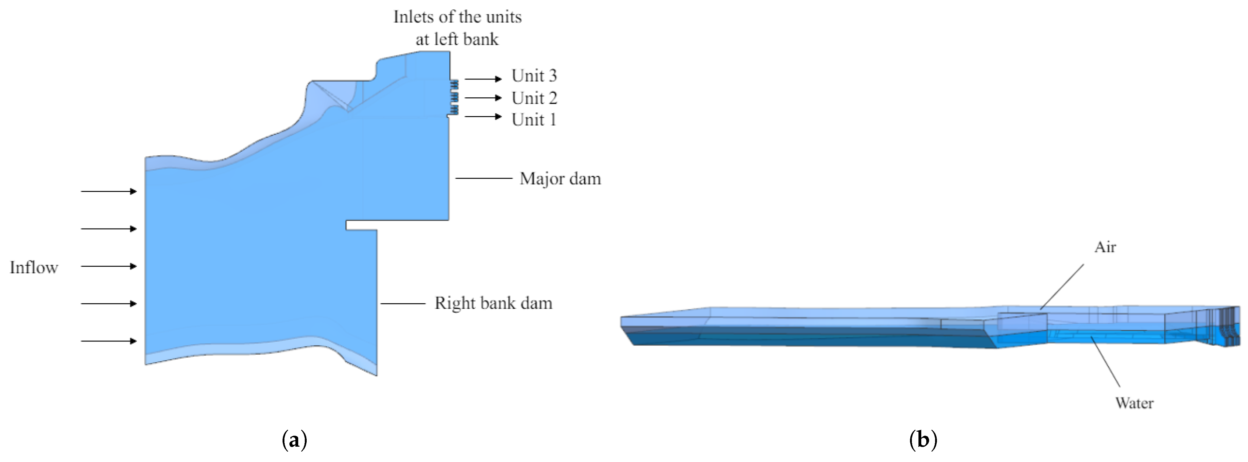
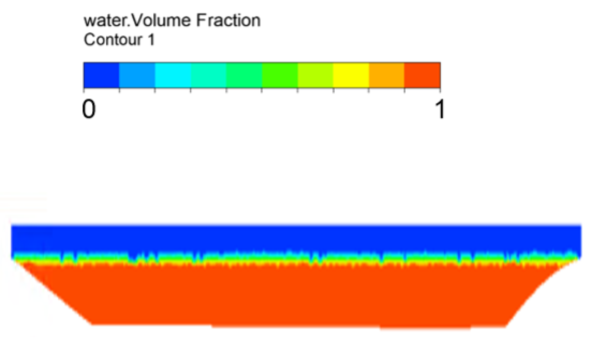
2.2. Calculation Model and Boundary Conditions

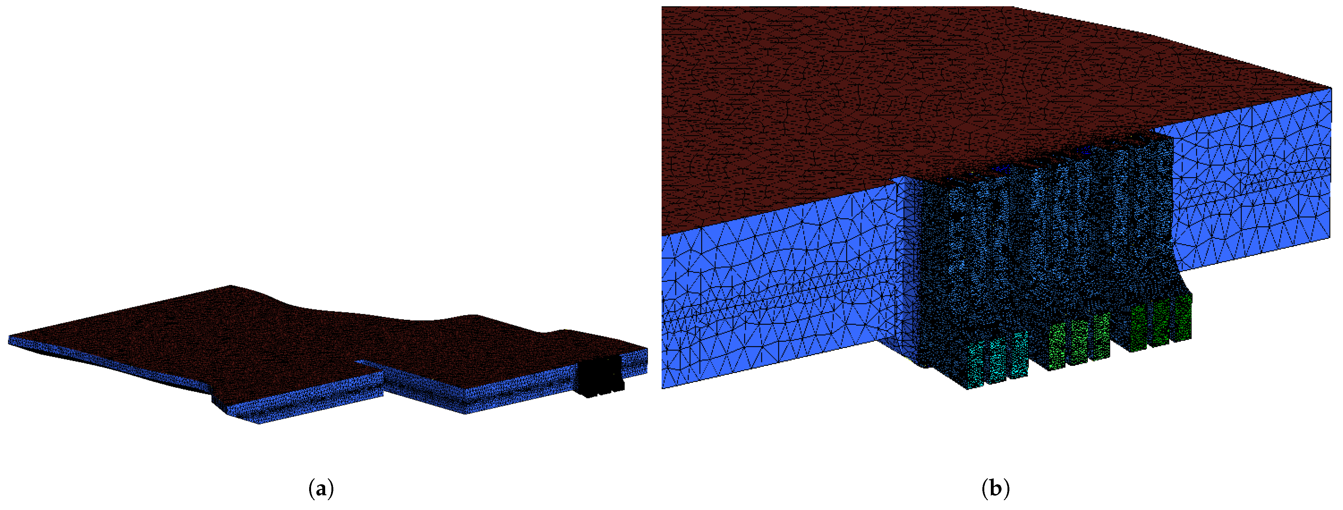
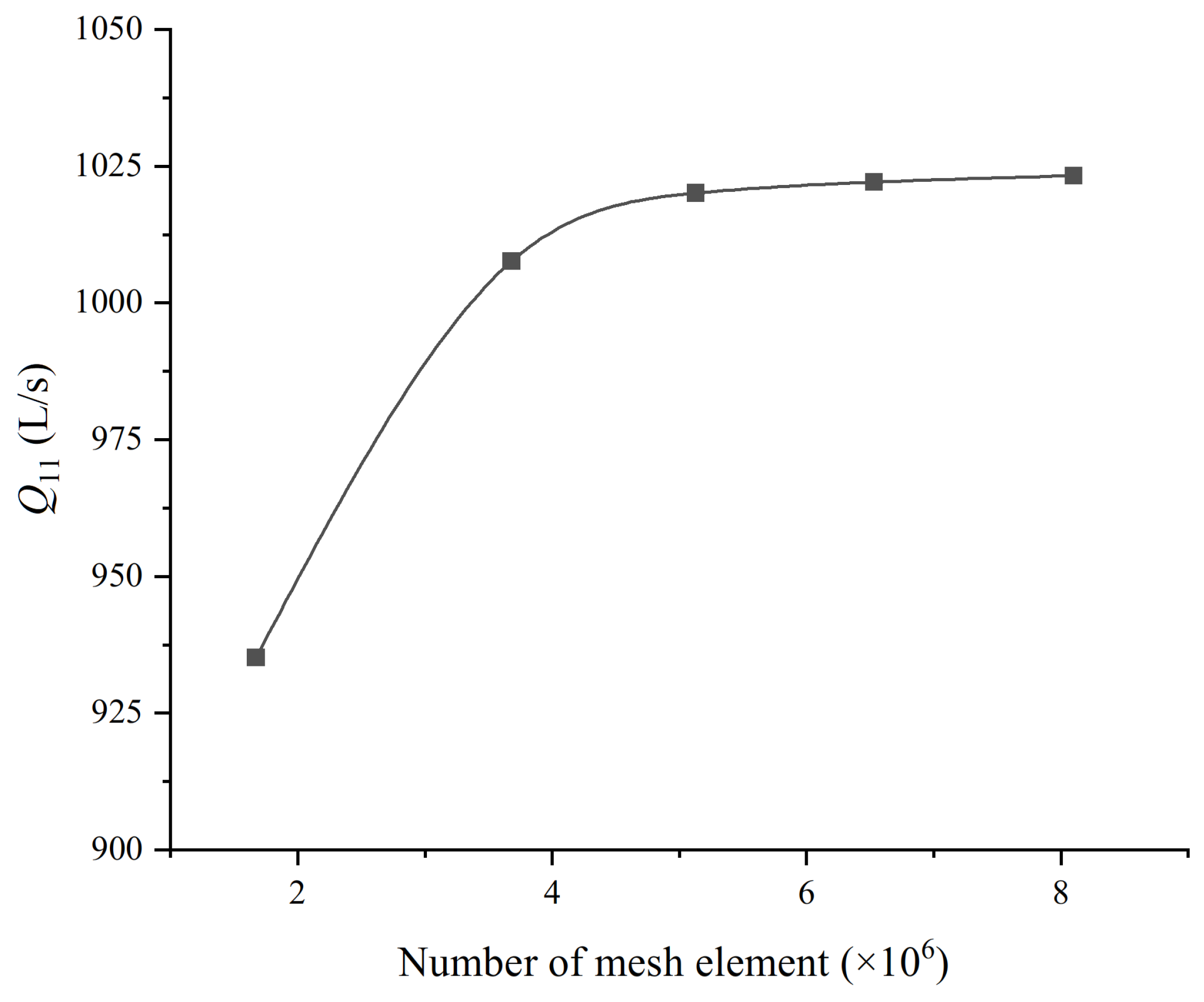
Generally speaking, the flow near the inlet section of the unit will be affected by the upstream flow, so it is necessary to consider the influence of the upstream river channel. The inlet section and upstream calculation domain of the three units on the left bank were established, as shown in Figure 1. After conducting free surface flow calculations, it was found that the streamlines in the upstream area (as shown in Figure 2) showed significant flow deviation and vortex characteristics only in the vicinity of the inlet section of the left bank unit, while in the upstream area far from the inlet section of the unit (upstream of straight line A-A), the streamlines are evenly distributed. Therefore, considering the limitations of computing resources, a local computing domain is established in this study, including the inlet section of the three units on the left bank and the surrounding area, as shown in Figure 3, including the air domain and the water domain. All simulation calculations are conducted in commercial software CFX.

According to different upstream water levels, the flow field is initialized using a CEL expression. Above the free liquid level is the air domain, with a gas phase volume fraction of 1 and a liquid phase volume fraction of 0. At the free liquid level, both gas and liquid phase volume fractions are 0.5, with a gas phase volume fraction of 1 and a liquid phase volume integral of 0, as shown in Figure 4.

Assuming that the flow at the inlet of the calculation domain in Figure 3 is uniform, the liquid phase velocity at the inlet is calculated from the flow rate and the cross-sectional area of the flow, as shown in Equation (7). VOF${}_w$ and VOF${}_a$ in Equations (8) and (9) are used to distinguish the air domain from the water domain, Ain is the cross-sectional area of the flow at the inlet, z is the vertical coordinate, and $H_{up}$ is the upstream water level; The outlet is the outlet cross-section of the inlet section of the three units on the left bank. Given the static pressure outlet conditions, the static pressure value is related to the water level, as shown in Equation (10), where $\rho$ is the density of water, and pref is 1, the atmospheric pressure. The upper surface is set as a constant open pressure boundary, allowing air to flow freely, with a pressure value of 1 atm absolute atmospheric pressure. In the computational domain, except for the inlet, outlet, and upper surface, all other surfaces are walls, including the riverbed, main dam, retaining dam, and walls on both sides, all given non-slip wall boundary conditions.

$$u_{in}=\frac{Q}{A_{in}}\ast \mathrm{VO}{\mathrm{F}}_w$$

(7)

$$\mathrm{VO}{\mathrm{F}}_w=1-\mathrm{VO}{\mathrm{F}}_a$$

(8)

$$\mathrm{VO}{\mathrm{F}}_a=\mathrm{step}(z-H_{up})/1)$$

(9)

$$p_{out}=\rho g(H_{up}-z)\ast \mathrm{VO}{{\mathrm{F}}_{\mathrm{water}}}_{\_\mathrm{initial}}+p_{ref}$$

(10)

2.3. Mesh Division

Considering the complex shape and irregular geometric shape of the upstream reservoir calculation domain, such as the riverbed and main dam wall, this study divides the calculation domain shown in Figure 3 into unstructured meshes, and increases the number of meshes in the inflow section of the unit. At the same time, according to different water level conditions, the number of local meshes near the free liquid level is increased, as shown in Figure 5.

Five different mesh density schemes are used for mesh partitioning to verify mesh independence. Except for different mesh densities, the five mesh schemes have the same mesh division method and calculation settings, including the same calculation model, boundary conditions, initial conditions, solver settings, and convergence conditions. The average flow rate of the three units on the left bank at the exit is used as the evaluation standard for mesh independence verification. To facilitate comparative analysis under different water head conditions, the unit flow rate $Q_{11}$ is defined as shown in Equation (11):

$$Q_{11}=\frac{1000Q}{D_1^2\sqrt{H}}$$

(11)

Among them, Q is the unit flow rate, in m${}^3$/s, $D_1$ is the nominal diameter of the unit runner, H is the working head, and the unit flow rate $Q_{11}$ is in L/s. Figure 6 shows the average unit flow of the three units on the left bank under different grid schemes under the working conditions of water level $H_{up}$ = 61 m, water head H = 37.79 m, and theoretical unit flow of $Q_{11-d}$ = 1023.56 L/s. It can be observed that when the mesh size is greater than 6.53 × After ${10}^6$, the average unit flow rate hardly changes as the number of meshes increases, so the selected mesh size is 6.53 × ${10}^6$ mesh scheme for subsequent calculations.

3. Results and Analysis

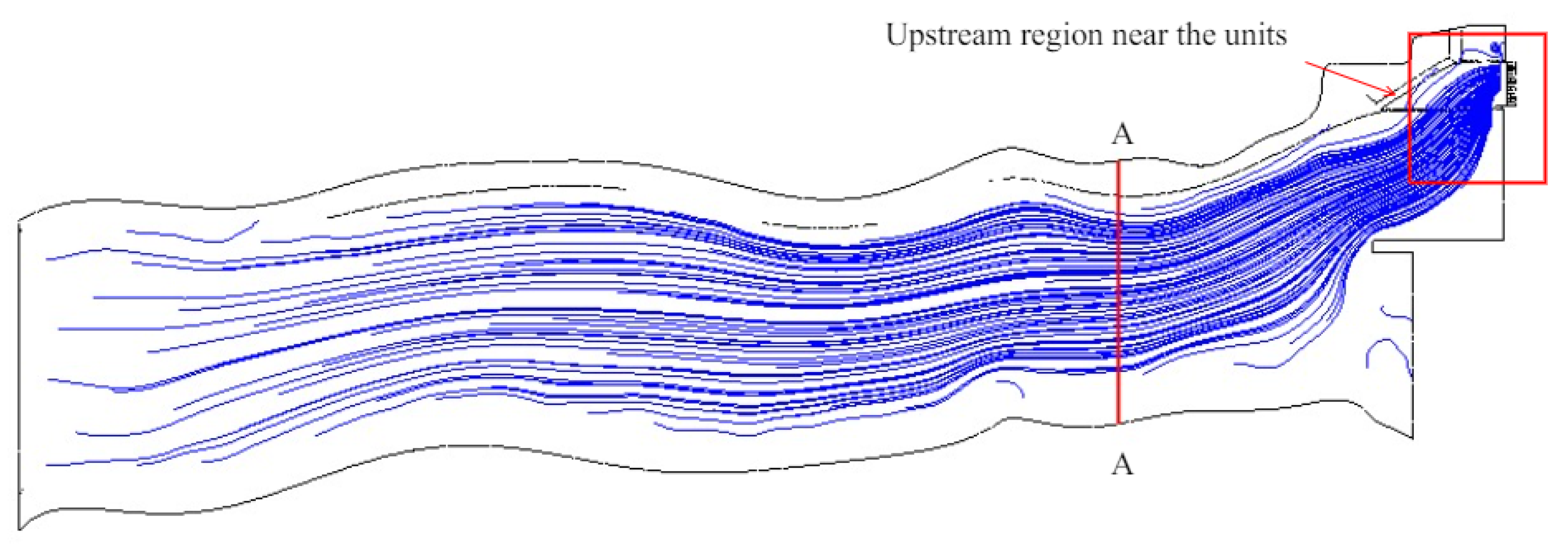
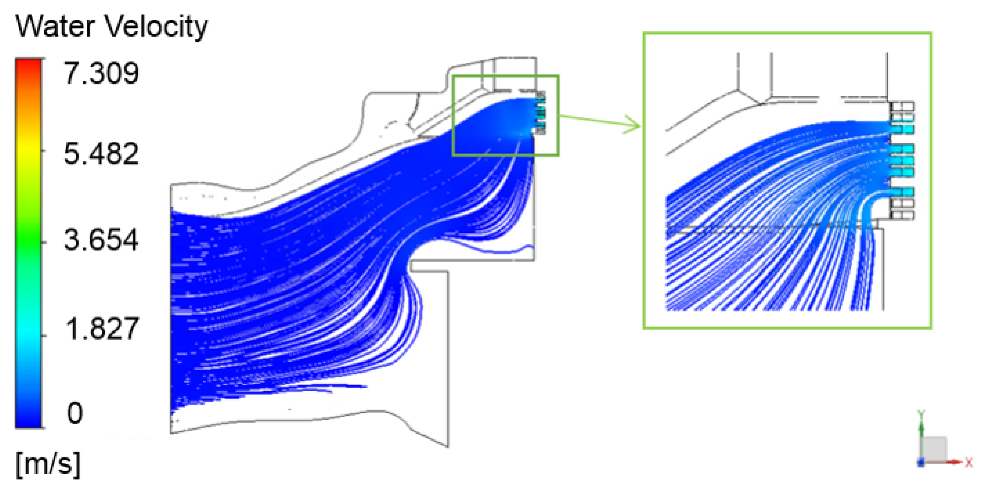
3.1. Impact of Upstream Reservoir Flow on Unit Flow

In this article, upstream water levels of 61 m, 55.67 m, 50.33 m, and 45 m are selected for analysis, and the operating parameters are shown in

Table 1. Main operating conditions parameters.

Upstream Water Level ${\mathit{H}}_{\mathit{up}}$ (m)	Condition	Unit Working Head H (m)	Ideal Unit Specific Discharge ${\mathit{Q}}_{11}$ (m${}^3$)
61	1	37.79	585.34
	2		805.12
	3		1023.56
55.67	4	31	660.17
	5		903.43
	6		1147.51
50.33	7	23.41	763.38
	8		1054.91
	9		1335.78
45	10	10.07	1033.45
	11		1624.93
	12		2053.18

.

Figure 7 shows the typical streamline distribution of the upstream reservoir under condition 8. It can be observed that there is a significant flow line deviation near the diversion wall between the main dam and the right bank retaining dam. At the same time, due to the influence of the left bank unit layout position, the flow line near the inlet of Unit 1 shows a deviation of nearly 90°, which is significantly different from the normal flow at the inlet of the unit under ideal conditions, and inevitably affects the hydraulic efficiency of the unit. Figure 2 shows the calculation domain containing the left bank three units inlet section and the upstream river area. The calculation results surface from the left bank unit inlet section far away from the region of the flow line is relatively smooth and uniform, basically the same direction as the river, in the unit inlet section of the guide wall in the vicinity of the region will produce obvious flow deflection and vortex characteristics. Due to the larger flow through the unit and the flow area of the upstream reservoir area being very large, the flow deflection phenomenon in the region near the guide wall is significantly stronger than the vortex characteristics; that is, compared to the overall flow deflection caused by the change in the geometric features of the river channel and the reservoir area, the vortex characteristics caused by the local corners play a significantly smaller role, and therefore, the overall flow line is shown as a deflection rather than a local vortex. The overall flowline features are chosen to be shown in both Figure 2 and Figure 7 to provide a visual understanding of the flow characteristics within the upstream reservoir area.

Figure 8 shows the unit flow of three units on the left bank under different water level conditions. Under different water level conditions, the unit flow of Unit 1 is significantly lower than that of Unit 2 and Unit 3. It can be observed that for low water level conditions, the difference in flow rate between Unit 1 and other units is more pronounced. For the Kaplan turbine, the flow rate has a significant impact on the output of the unit. The uneven distribution of flow in the upstream reservoir significantly reduces the flow rate of Unit 1, which is very detrimental to the output of the unit.

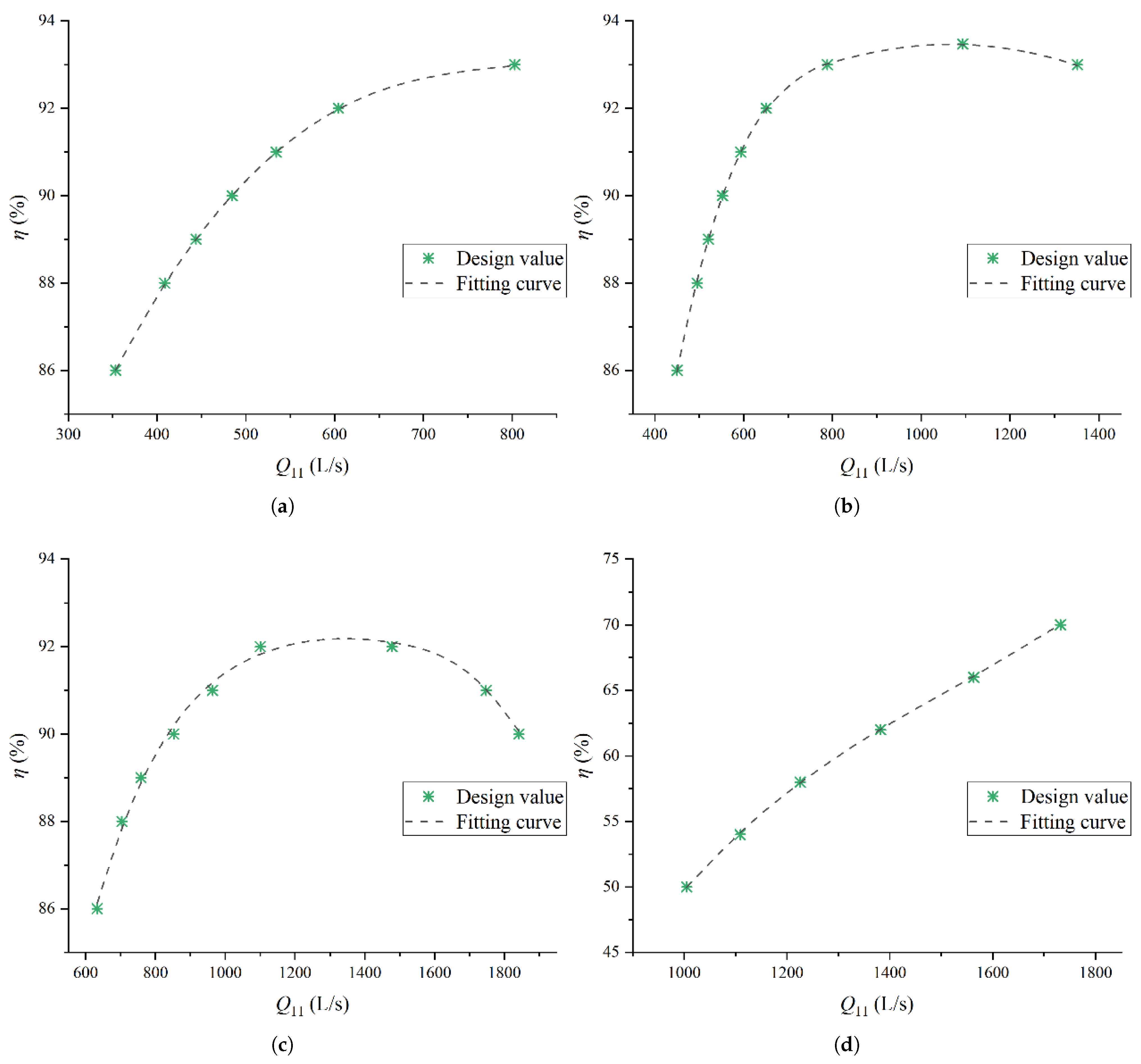
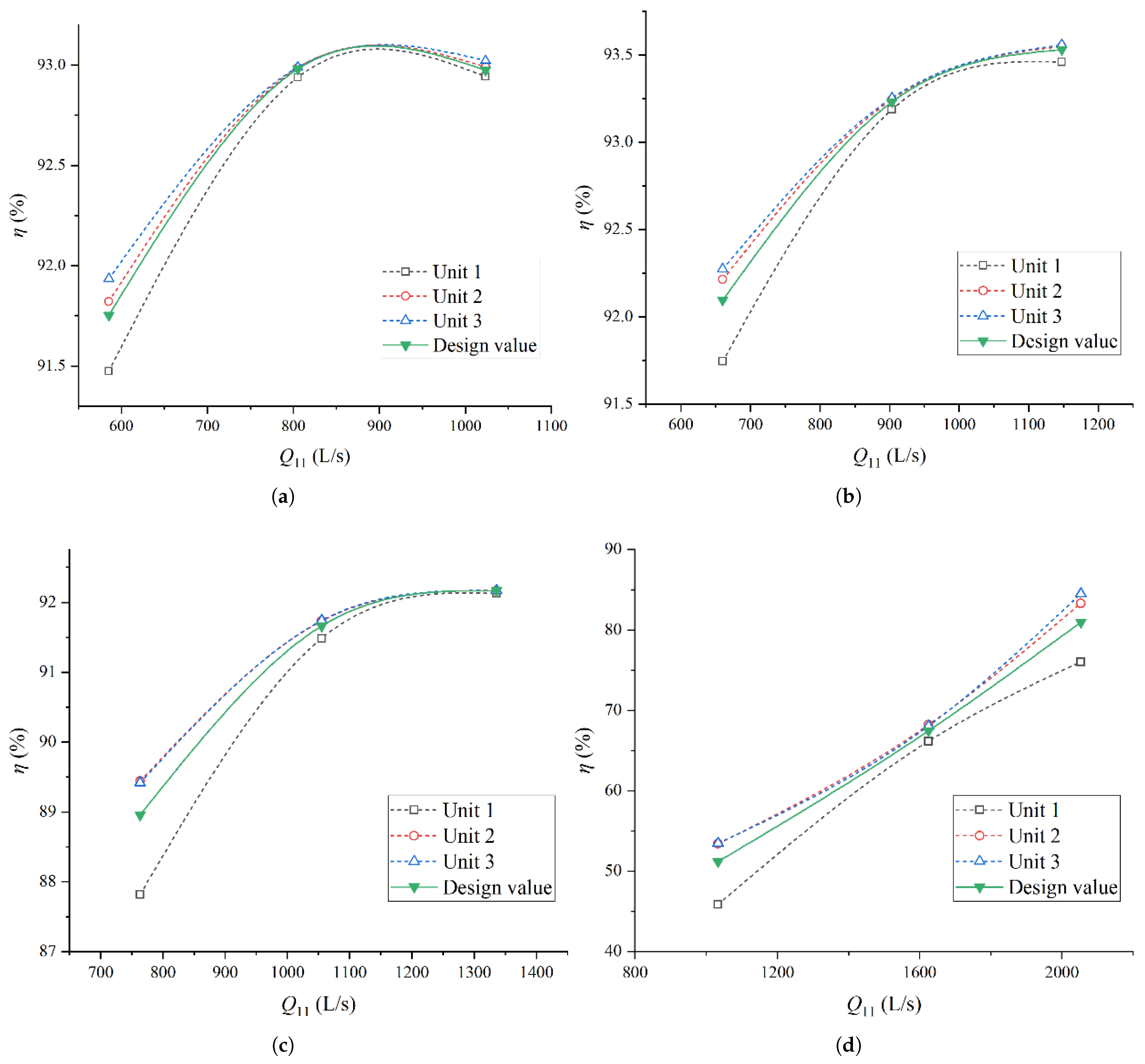
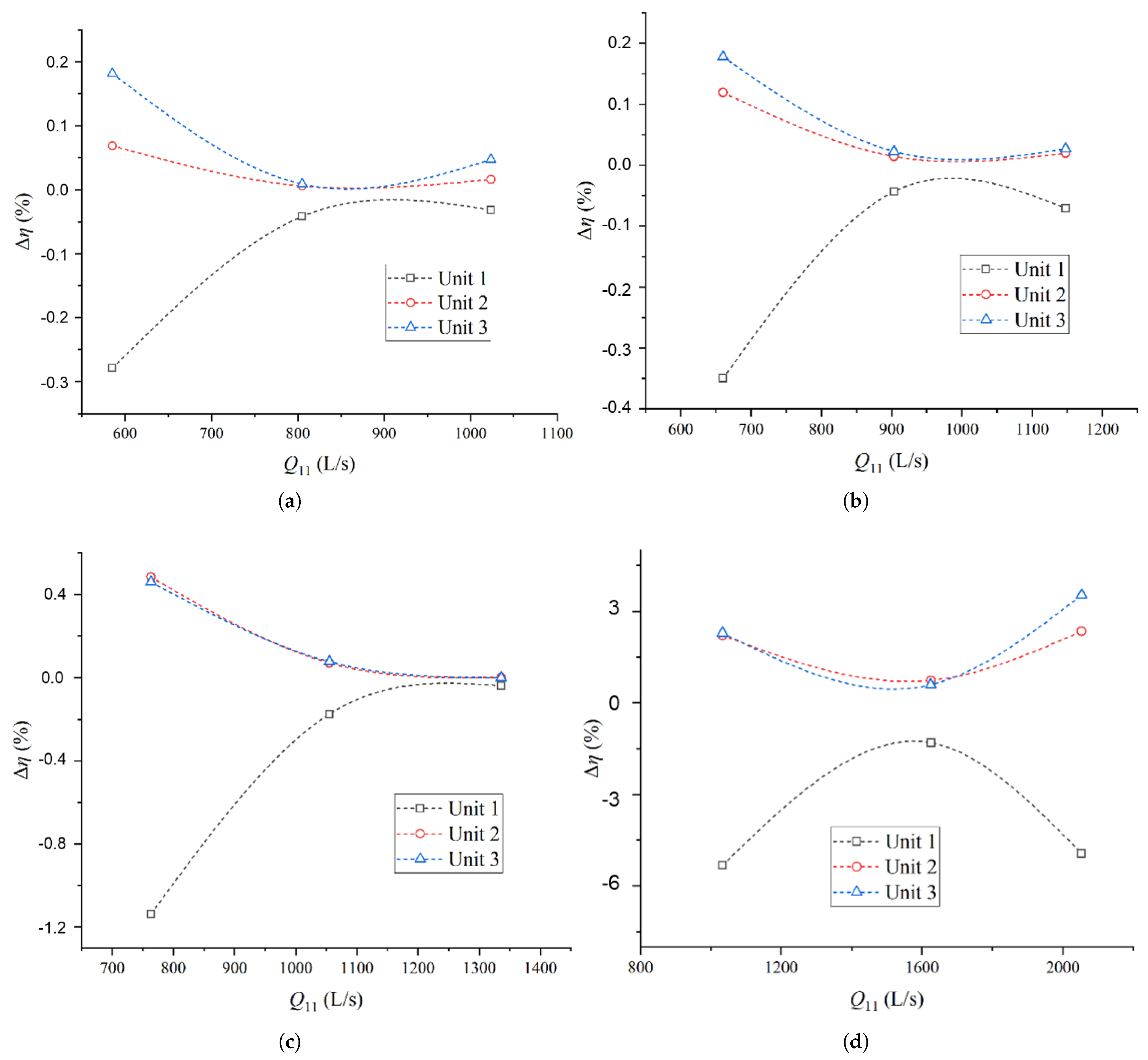
3.2. Impact of Upstream Reservoir Flow on Unit Efficiency

To estimate the impact of flow distribution in the upstream reservoir on the operational efficiency of the unit, this section first fits the relationship curve between unit efficiency and unit flow under different water head conditions based on the comprehensive characteristic curve of the model unit, as shown in Figure 9. The star-shaped scatter points in the figure represent the unit efficiency value calculated with the comprehensive characteristic curve, while the dashed line represents the polynomial fitting curve, and its fitting expression is:

$$\eta =a{Q}_{11}^4+b{Q}_{11}^3+c{Q}_{11}^2+d{Q}_{11}+e$$

(12)

Among them, a, b, c, d, and e are the fitting parameters, and their values are shown in

Table 2. Fitting parameters of the relationship curve between unit efficiency and unit flow rate.

Upstream Water Level ${\mathit{H}}_{\mathit{up}}$ (m)	a	b	c	d	e
37.79	-	4.424 × ${10}^{-10}$	−1.196 × ${10}^{-6}$	1.072 × ${10}^{-6}$	0.6111
31	−7.733 × ${10}^{-13}$	3.117 × ${10}^{-9}$	−4.686 × ${10}^{-6}$	3.126 × ${10}^{-3}$	0.1496
23.41	−1.525 × ${10}^{-13}$	8.127 × ${10}^{-10}$	−1.67 × ${10}^{-6}$	1.567 × ${10}^{-3}$	0.3568
10.07	-	2.765 × ${10}^{-10}$	−1.263 × ${10}^{-6}$	2.143 × ${10}^{-3}$	−0.659

.

Based on the above fitting relationship and the flow rate of the three units, the efficiency of the three units under different water level conditions is interpolated and estimated, as shown in Figure 10. The dashed line represents the estimated efficiency of the three units, and the solid line represents the ideal efficiency value of the units. It can be observed that after considering the influence of the upstream reservoir, the efficiency of the three units follows the same trend as the ideal situation in terms of unit flow. However, under the same unit flow conditions, the efficiency curves of Unit 2 and Unit 3 are higher than the ideal situation, while the efficiency curves of Unit 1 are lower than the ideal situation. The estimated values of efficiency $\eta$ versus unit flow $Q_{11}$ for the three units on the left bank at the upstream water level $H_{up}$ = 61 m and working head H = 37.79 m are shown in Figure 10a. The efficiency values are basically the same near $Q_{11}$ = 800 L/s and near $Q_{11}$ = 1020 L/s, while the maximum value exists near $Q_{11}$ = 900 L/s, which is mainly due to the fact that its highest efficiency point is near that unit speed. Combining the efficiency curves of the unit in the design case reveals that there is also a significant maximum near the unit speed $Q_{11}$ = 900 L/s. This indicates that the unit’s highest efficiency point (BEP, Best Efficient Point) is near that unit speed under the design condition and that operating head condition, so even though there is some deviation in the efficiency values of the three units under the influence of the upstream reservoir, their BEPs are still near the unit speed $Q_{11}$ = 900 L/s.

Figure 11 shows the difference between the estimated and designed efficiency values of the three units on the left bank under different water level conditions. It can be observed that due to the uneven distribution of flow in the upstream reservoir, under the same water level and inflow conditions, the passing flow of Unit 1 is significantly lower than the design value. This causes the operating point of the unit to deviate from the cam-coordinate point under the inflow conditions, and the efficiency of the unit is significantly lower than the design value. At low water levels ($H_{up}$ = 45 m), it is very obvious that when the unit flow rate of the unit is low, the decrease in efficiency relative to the design value exceeds 5%. This means that the upstream reservoir flow has a more significant impact on the operational efficiency of the unit under low water levels.

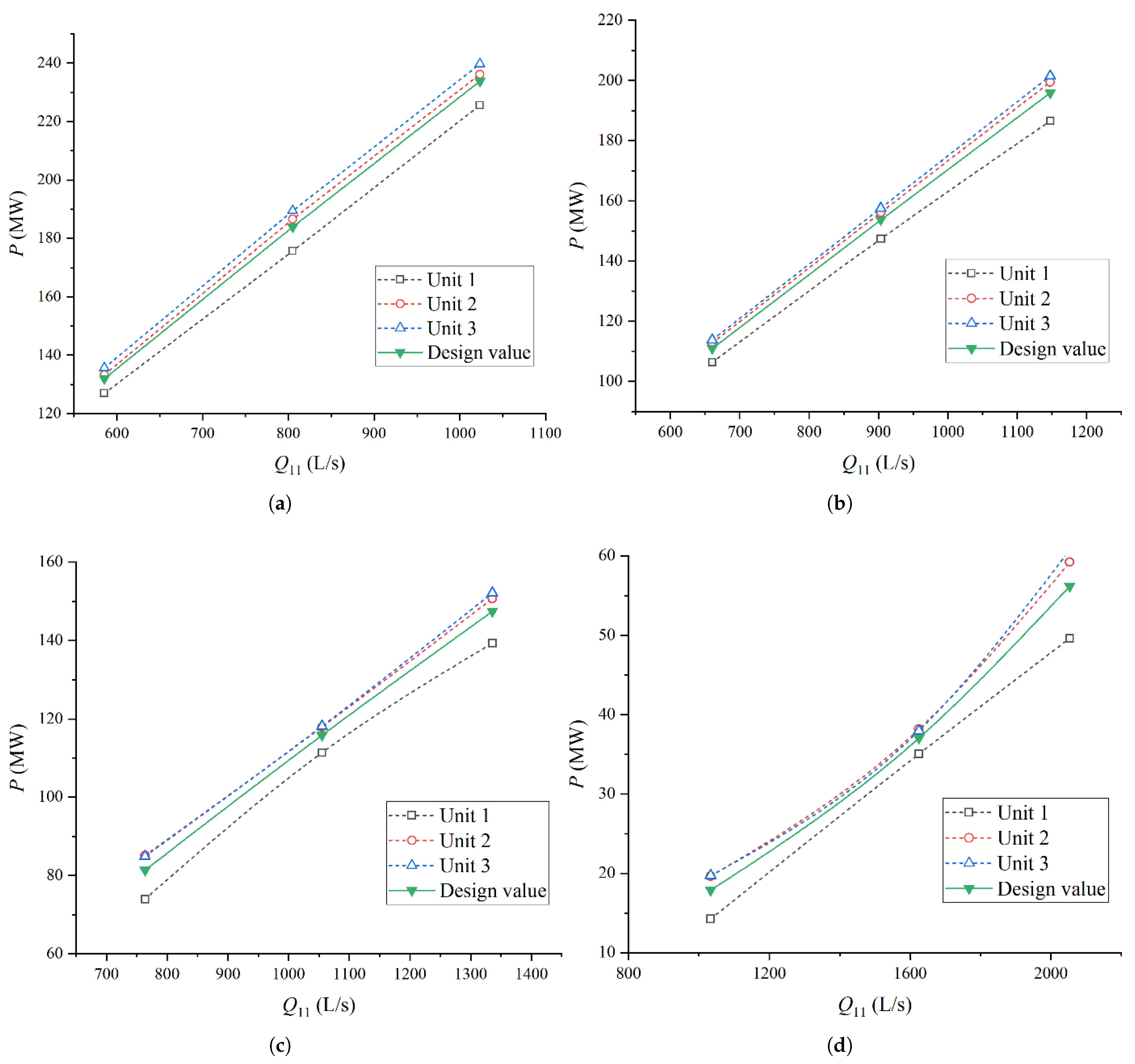
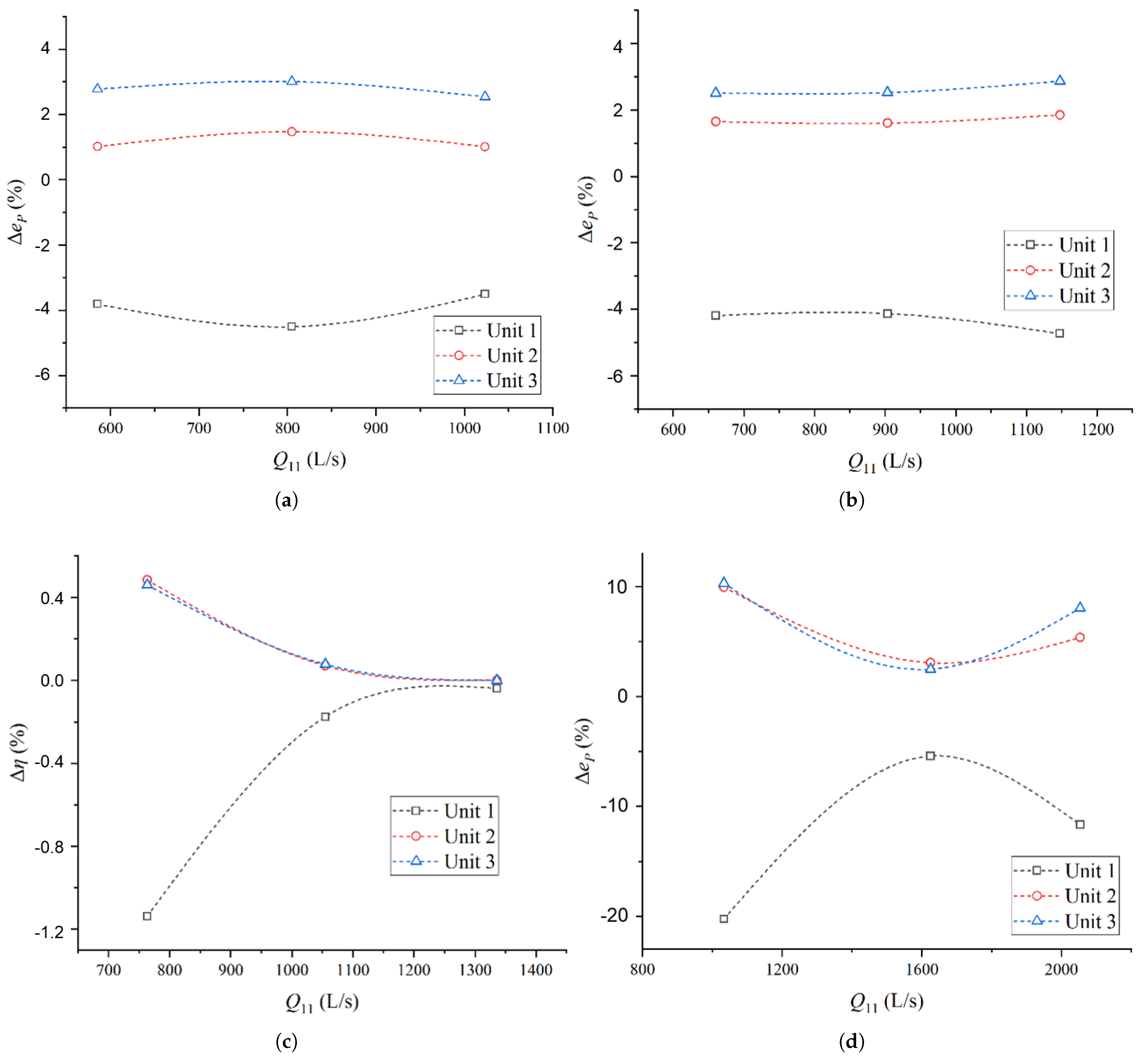
3.3. Impact of Upstream Reservoir Flow on Unit Output

Based on the estimated flow rates of the three units in Section 3.1 and the unit efficiency in Section 3.2, the relationship curve between the output of the three units on the left bank under different water level conditions and the unit flow rate can be calculated, as shown in Figure 12, where the power P is calculated as:

$$P=\frac{\rho gQH\eta }{{10}^6}$$

(13)

From Figure 8, it can be seen that the flow rate curve of Unit 1 is significantly lower than that of Unit 2 and Unit 3. From Figure 10, it can be seen that the efficiency curve of Unit 1 is significantly lower than that of the other units. Therefore, the estimated output curve of Unit 1 is also significantly lower than that of the other units.

Figure 13 shows the difference $e_p$ between the output of the three units and the design value, defined as:

$$e_P=\frac{P-P_d}{P_d}\times 100\%$$

(14)

where P is the unit power and $P_d$ is the design value of the unit output. It can be observed that under different operating conditions, the decrease in output of Unit 1 relative to the design value is greater than 3%. At low water levels ($H_{up}$ = 45 m), when the unit flow rate of the unit is low, the decrease in output relative to the design value can even reach 20%, which is consistent with the phenomenon observed during actual operation on site. When Unit 1 operates under different water head conditions, its output is lower than the other two units, especially when the upstream water level is low, the output value significantly decreases.

4. Conclusions

In this article, the VOF method is used to numerically simulate the upstream reservoir flow of a giant axial flow turbine, and the impact of the model unit’s comprehensive characteristic curve on the upstream reservoir flow is analyzed. Through the evaluation and analysis of the flow rate, efficiency, and output of the three units on the left bank under different water level conditions, the following conclusions are drawn:

• Due to the influence of the layout position of the left bank unit, there is a significant deviation of streamlines near the inlet of Unit 1, which is significantly different from the normal flow at the inlet of Unit 1 under ideal conditions. As a result, the flow rate of Unit 1 under the same water level conditions is significantly lower than that of Unit 2 and Unit 3.
• Based on the relationship curve between unit efficiency and unit flow, the estimated efficiency values of the three units on the left bank under different water level conditions are obtained through interpolation. It can be found that due to the uneven distribution of flow in the upstream reservoir area, the efficiency of Unit 1 is significantly lower than the design value under the same water level and inflow conditions, especially when the efficiency drops by more than 5% under low water level conditions.
• Comparing the output of three units on the left bank under different water level conditions, it is found that the decrease in output of Unit 1 compared to the design value is greater than 3%, and even reaches 20% under low water level conditions. This is consistent with the phenomenon observed during actual operation on site.

References

1. Lichtneger, P. Intake flow problems at low-head hydropower. Dresdner Wasserbauliche Mitteilungen 2009, 39, 259–266. [Google Scholar]
2. Suerich-Gulick, F.; Gaskin, S.J.; Marc, V.; Étienne, P. Characteristics of free surface vortices at low-head hydropower intakes. J. Hydraul. Eng. 2014, 140, 291–299. [Google Scholar] [CrossRef]
3. Amiri, K.; Mulu, B.; Raisee, M. Effects of upstream flow conditions on runner pressure fluctuations. J. Appl. Fluid Mech. 2017, 10, 1045–1059. [Google Scholar] [CrossRef]
4. Ahn, S.H.; Xiao, Y.X.; Wang, Z.W. Numerical prediction on the effect of free surface vortex on intake flow characteristics for tidal power station. Renew. Energy 2017, 101, 617–628. [Google Scholar] [CrossRef]
5. Deng, Y.C. Study on the Characteristics and the Critical Submergence of Vortex in Multi-Level Stop-Log Gates Intake of Hydropower Stations; Xi’an University of Technology: Xi’an, China, 2019. [Google Scholar]
6. Dang, Y.Y.; Han, C.H. Review of vortexes at intakes. Adv. Sci. Technol. Water Resour. 2009, 29, 90–94. [Google Scholar]
7. Hattersley, R.T. Hydraulic design of pump intakes. J. Hydraul. Div. 1965, 91, 223–249. [Google Scholar] [CrossRef]
8. Dicmas, J.L. Effect of intake structure modifications on the hydraulic performance of a mixed flow pump. In Proceedings of the IAHR, ASME, and ASCE Joint Symposium on Design and Operation of Fluid Machinery; Colorado State University: Fort Collins, CO, USA, 1978; Volume 1, pp. 403–412. [Google Scholar]
9. Vermeyen, T.B. Glen Canyon Dam Multi-Level Intake Structure Hydraulic Model Study; Water Resources Services, Water Resources Research Laboratory, Technical Service Center: Denver, CO, USA, 1999. [Google Scholar]
10. Vermeyen, T.B. An overview of the design concept and hydraulic modeling of the Glen Canyon Dam Multi-Level intake structure. In Proceedings of the Waterpower’99 Conference, Las Vegas, NV, USA, 6–9 July 1999. [Google Scholar]
11. Forkel, C.; Jokiel, C.; Bergen, O. Model and Numerical Simulations for the intake works of Bakun Reservior. J. Hydropower Dams 1996, 6. [Google Scholar]
12. Rettemeier, K.; Demny, G.; Forkel, C. Verification of the simulated 3D flow through intake of a river run power plant. Hydroinformatics 1998, 2, 1433–1439. [Google Scholar]
13. Sarkardeh, H.; Reza Zarrati, A.; Jabbari, E. Numerical simulation and analysis of flow in a reservoir in the presence of vortex. Eng. Appl. Comput. Fluid Mech. 2014, 8, 598–608. [Google Scholar] [CrossRef]
14. Kim, C.G.; Choi, Y.D.; Choi, J.W. A study on the effectiveness of an anti vortex device in the sump model by experiment and CFD. Iop Conf. Ser. Earth Environ. Sci. 2012, 15, 072004. [Google Scholar] [CrossRef]
15. Li, H.; Chen, H.; Ma, Z. Formation and influencing factors of free surface vortex in a barrel with a central orifice at bottom. J. Hydrodyn. 2009, 21, 238–244. [Google Scholar] [CrossRef]
16. Okamura, T.; Kamemoto, K.; Matsui, J. CFD prediction and model experiment on suction vortices in pump sump. In Proceedings of the 9th Asian International Conference on Fluid Machinery, Jeju, Republic of Korea, 16–19 October 2007; pp. 16–19. [Google Scholar]
17. Suerich-Gulick, F.; Gaskin, S.; Villeneuve, M. Experimental and numerical analysis of free surface vortices at a hydropower intake. In Proceedings of the 7th International Conference on Hydroscience and Engineering, Philadelphia, PA, USA, 10–13 September 2006; pp. 1–11. [Google Scholar]
18. Brocard, D.N.; Beauchamp, C.H.; Hecker, G.E. Analytic Predictions of Circulation and Vortices at Intakes; Electric Power Research Institute Project; EPRI: Holden, MA, USA, 1982; pp. 1199–1208. [Google Scholar]
19. Constantinescu, G.S.; Patel, V.C. Numerical model for simulation of pump-intake flow and vortices. J. Hydraul. Eng. 1998, 124, 123–134. [Google Scholar] [CrossRef]
20. Zhao, Y.Z.; Gu, Z.L.; Yu, Y.Z. Numerical analysis and structure of evolution of free water vortex. J. Xi’an Jiaotong Univ. 2003, 37, 85–88. [Google Scholar]
21. Lei, Y. Research on Numerical Simulation of Turbulent Flow for Stratified Intake in Hydropower Staion; Wuhan University: Wuhan, China, 2010. [Google Scholar]
22. Hirt, C.W.; Nichols, B.D. Volume of fluid (VOF) method for the dynamics of free boundaries. J. Comput. Phys. 1981, 39, 201–225. [Google Scholar] [CrossRef]
23. Rudman, M. Volume-tracking methods for interfacial flow calculations. Int. J. Numer. Methods Fluids 1997, 24, 671–691. [Google Scholar] [CrossRef]
24. Menter, F.R. Two-equation eddy-viscosity turbulence models for engineering applications. AIAA J. 1994, 32, 1598–1605. [Google Scholar] [CrossRef]
25. Wilcox, D.C. Reassessment of the scale-determining equation for advanced turbulence models. AIAA J. 1988, 26, 1299–1310. [Google Scholar] [CrossRef]
26. Launder, B.E.; Sharma, B.I. Application of the energy-dissipation model of turbulence to the calculation of flow near a spinning disc. Lett. Heat Mass Transf. 1974, 1, 131–137. [Google Scholar] [CrossRef]
Figure 1. Calculation domain of upstream reservoir, including river channel.
Water 15 03920 g001
Figure 2. Flow line distribution in upstream reservoir.
Water 15 03920 g002
Figure 3. Local calculation domain of free surface flow in upstream reservoir. (a) Cross Section. (b) Fluid distribution.
Water 15 03920 g003
Figure 4. Initialization of free surface flow field.
Water 15 03920 g004
Figure 5. Mesh division. (a) Meshes of the overall model. (b) Meshes near the inlet section of the unit.
Water 15 03920 g005
Figure 6. Variation of unit average unit flow with number of meshes.
Water 15 03920 g006
Figure 7. Typical streamline distribution of upstream reservoirs.
Water 15 03920 g007
Figure 8. Unit flow of three units on the left bank under different water level conditions. (a) H u p = 61 m. (b) H u p = 55.67 m. (c) H u p = 50.33 m. (d) H u p = 45 m.
Water 15 03920 g008
Figure 9. Relationship between unit efficiency and unit flow under different water level conditions. (a) H u p = 61 m. (b) H u p = 55.67 m. (c) H u p = 50.33 m. (d) H u p = 45 m.
Water 15 03920 g009
Figure 10. Estimated efficiency values of three units on the left bank under different water level conditions. (a) H u p = 61 m. (b) H u p = 55.67 m. (c) H u p = 50.33 m. (d) H u p = 45 m.
Water 15 03920 g010
Figure 11. Difference between the estimated and designed efficiency values of the three units on the left bank under different water level conditions. (a) H u p = 61 m. (b) H u p = 55.67 m. (c) H u p = 50.33 m. (d) H u p = 45 m.
Water 15 03920 g011
Figure 12. Estimated output values of three units on the left bank under different water level conditions. (a) H u p = 61 m. (b) H u p = 55.67 m. (c) H u p = 50.33 m. (d) H u p = 45 m.
Water 15 03920 g012
Figure 13. Relative difference between estimated output values and design values of three units on the left bank under different water level conditions. (a) H u p = 61 m. (b) H u p = 55.67 m. (c) H u p = 50.33 m. (d) H u p = 45 m.
Water 15 03920 g013