Space-Time Variability of Drought Characteristics in Pernambuco, Brazil

Abstract

Drought is the most complex natural hazard that can occur over large spatial scales and during long time periods. It affects more people than any other natural hazard, particularly in areas with a dry climate, such as the semiarid region of the Brazilian Northeast (NEB), which is the world’s most populated dry area. In this work, we analyzed trends and the spatial distribution of drought characteristics (frequency, affected area, and intensity) based on the Standardized Precipitation Index (SPI) on annual (SPI-12) and seasonal (SPI-3) scales. The study used monthly precipitation data recorded between 1962 and 2012 at 133 meteorological stations in Pernambuco State, Brazil, which is located in the eastern part of the NEB and has more than 80% of its territory characterized by a semiarid climate. The regions of Sertão, Agreste, and Zona da Mata of Pernambuco were considered for comparison. The Mann–Kendall and Sen’s slope tests were used to detect the trend and determine its magnitude, respectively. The results indicated that annual droughts in the state of Pernambuco became more frequent from the 1990s onwards, with summer having the greatest spatial coverage, followed by winter, autumn, and spring. Sertão presented a greater number of stations with a significant positive trend in drought frequency. Regarding the drought-affected area, global events occurred in a greater number of years on an annual scale and during the summer. Trend analysis pointed to an increase in areas with drought events on both scales. As for the drought intensity, the entire state of Pernambuco experienced drought events with high intensity during the autumn. The relationship between drought characteristics indicated an increase in the affected area as the result of an increase in drought intensity.

1. Introduction

Drought has been considered one of the most complex and least understood natural disasters in the world [1]. The phenomenon has affected more people than other natural hazards such as floods and tropical cyclones [2,3], for example. According to the World Meteorological Organization (WMO) [4], during the period from 1970 to 2019, drought was the natural disaster that generated the most losses of human lives. Sena et al. [5] reported that, between 1960 and 2013, there were about 612 drought events, which resulted in more than two million deaths and affected more than two billion people. There are records of devastating drought events that caused millions of deaths in Europe, the United States, Russia, China, and Africa in the 20th and 21st centuries [6,7]. In addition to death from starvation, droughts can also be linked to many other social and public health problems, as reported in recent years [8,9,10,11].

In addition to the numerous impacts it has on social life, the drought phenomenon is the natural disaster that generates the most costs to the global economy [12]. The agricultural sector is the most affected, although other sectors such as tourism, transport, and energy production can also suffer considerable impacts [13]. Arid and semi-arid regions are the most sensitive to the impacts of drought events [14] and are also the regions where droughts occur more frequently, affecting their livelihoods and sustainable development [15].

Analyzing drought is not an easy task, mainly because it is a phenomenon that can occur in areas of both high and low precipitation [16] and over short periods, such as weeks or months, or long periods, such as seasons, years, or decades [17]. Another challenge is knowing which type of drought should be investigated. Wilhite and Glantz [16] define at least four types of droughts: meteorological, agricultural, hydrological, and socioeconomic. Meteorological droughts can be defined based on the degree of dryness and the length of a dry period and, similar to the other three types of droughts, happen due to a lack of rainfall. The climatological variable considered in the analysis of meteorological droughts is, therefore, precipitation [18]. Awchi and Kalyana [19] explain that prolonged meteorological droughts can be the cause of other droughts, such as agricultural droughts (caused by soil moisture deficits), that harm agricultural production and, afterward, generate socioeconomic droughts, affecting human life. In addition, meteorological droughts may be followed by hydrological droughts, which, according to [20], are related to a lack of water in hydrological systems, generating low and abnormal flows in rivers and low levels in underground reservoirs and lakes.

According to Marengo et al. [21], the semi-arid region of the Brazilian Northeast (NEB) is possibly the most vulnerable to dry events. The history of droughts in northeastern Brazil dates back to the 16th century and continued during the 18th, 19th, and 20th centuries [22,23]. The results of recent paleoclimatic studies suggest that NEB experienced cycles of long humid and dry periods during the last 2300 years: a predominantly humid period between 500 years BCE and 420 years CE, followed by an abrupt aridification and a long dry period from 500 to 1300 years CE, and a humid period between 1580 and 1900 years CE [24]. Among the droughts registered in the 19th century, the worst case so far occurred from 1877 to 1879 in the Brazilian semiarid region, affecting the entire Northeast region and causing around 200,000 to 500,000 deaths, as estimations reported in [25]. The droughts recorded in the 20th century occurred in the following periods: (i) between 1903 and 1904, causing a new rural exodus in the Northeast region; (ii) between 1914 and 1915, causing more than 278,000 deaths; (iii) in 1958, affecting about 10 million people; (iv) from 1979 to 1984 (dry period of greater scope), leaving thousands of people in hunger and misery, primarily in the years 1982 and 1983, which registered an 80% drop in livestock and affected almost 29 million people; (v) between 1986 and 1988, which affected the region but with less intensity [26]; (vi) from 1990 to 1995 (1993 being the driest year); and (vii) from 1997 to 1999. In the 21st century, droughts occurred between 2012 and 2018, reaching 98.7% of the northeastern municipalities and making the São Francisco River reach a level reduction never observed before or after this period. Drought events were observed during El Ninho (1998, 2002, and 2015–2016), La Nina (2011–2012), and the 2012–2018 drought was related to a warmer tropical North Atlantic (and reinforced by an El Nino event in 2016) [21,26]. A recent study based on the nonlinear phase coherence and event synchronization analysis of sea surface temperature (SST) in the North Atlantic and Pacific oceans and the standardized precipitation index (SPI) in the NEB showed that tropical North Atlantic plays the dominant role for precipitation variability and that the indirect Pacific-North Atlantic phase synchronizations have a significant influence on the development and reinforcement of the droughts in the NEB [27].

The techniques used to identify and investigate dry events involve the calculation of indices that work as drought indicators and are based on daily or monthly records of climatic variables such as precipitation, evaporation, and temperature—the first two variables being the most used, according to [28]. Other indexes consider both precipitation and temperature in their calculations [29,30]. As reported in [31], several indices can identify meteorological droughts based on precipitation data [32,33,34,35,36,37,38,39] or precipitation together with other meteorological variables. According to Wang et al. [40] and Jain et al. [41], the Standardized Precipitation Index—SPI [39] is one of the most used drought indicators in the analysis of meteorological, hydrological, and agricultural droughts. The calculation of SPI considers spatial and temporal standardization, allowing for determining how rare a drought event is and how much precipitation is needed to eliminate the drought in any part of the world [42]. In addition, SPI is the index highlighted by the World Meteorological Organization as a starting point for meteorological drought monitoring [31].

The SPI indicator by itself is not sufficient to extract drought information. However, from the time series of SPI values, it is possible to obtain characteristics of drought events through the theory of runs proposed by [42]. In addition, a more in-depth investigation that also aims to collect useful information for the development and management of water resources in the studied region should include a space-time analysis, that is, a spatial and trend analysis of precipitation and the drought characteristics to make predictions and estimations of their spatial distributions, respectively [43,44]. Temporal analysis is commonly performed using statistical tests, while spatial analysis uses geostatistical methods [45,46].

Aiming to better understand the characteristics of regional drought and to provide a reference for drought disaster reduction and improved water resource management in Pernambuco, a state of NEB, this study used the SPI and its derived drought frequency, affected area, and drought intensity as the analysis parameters of the spatial-temporal distribution of meteorological drought. There are only a few studies that concentrate on drought conditions in Pernambuco. Souza et al. [47] analyzed drought conditions in Pernambuco based on soil moisture anomalies (using data from the Soil Moisture and Ocean Salinity—SMOS satellite) for the period 2010–2017 and identified the dry period between 2012 and 2017, with 2012 being the driest year. Inocêncio et al. [48] used several standardized climate indices to study drought characteristics in five river basins located in Pernambuco and found that events between 2012 and 2017 had more severe SSMI (Standardized Soil Moisture Index) and SSI (Standardized Streamflow Index) values than SPI (Standardized Precipitation Index) and SPEI (Standardized Precipitation Evapotranspiration Index). Silva et al. [49] investigated the spatiotemporal variability of rainfall in Pernambuco based on daily rainfall data from 38 weather stations for the period 1990–2020. They used several climate indices, among them the Standardized Precipitation Index (SPI) to assess drought conditions across the state mesoregions. The SPI-12 values indicated that the most severe and widespread droughts occurred during the 1990s and 2010s, except in the semiarid Sertão do São Francisco mesoregion, where they were predominant in the 2010s. Drought characteristics in the studied area were also reported in large-scale studies that included NEB [26,50,51], semiarid NEB [21,52], and the entire Brazilian territory [53]. In this work, we investigated drought conditions in Pernambuco through a comprehensive analysis of the Standardized Precipitation Index on annual (SPI-12) and seasonal (SPI-3) scales, based on the measured data from 133 weather stations in Pernambuco from 1959 to 2013. In addition, we evaluated the relationship between the drought-affected areas and drought intensity. The findings of this study offer valuable insights into the dynamics of drought in Pernambuco, with implications for effective drought management strategies and sustainable water resource practices in the region.

2. Materials and Methods

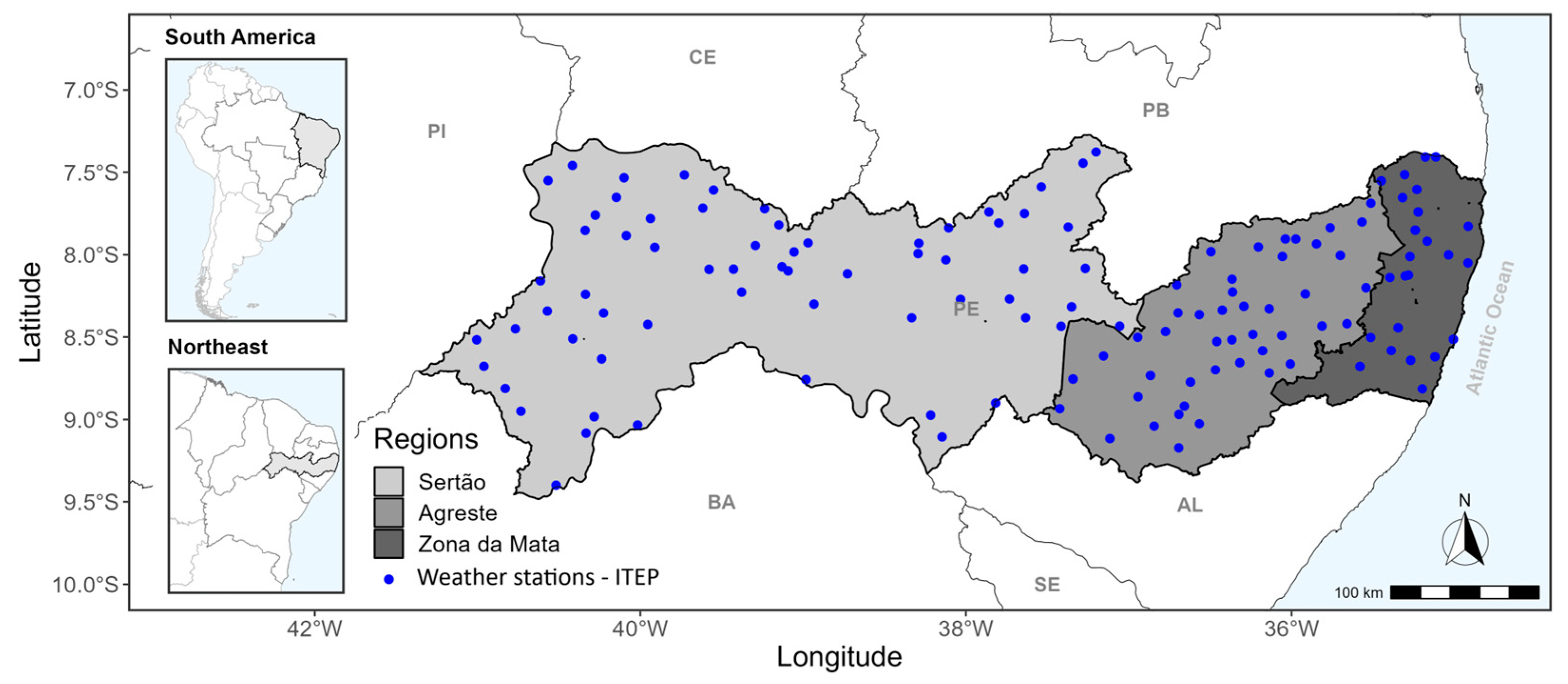
2.1. Study Area and Dataset

The region under analysis is the state of Pernambuco, which is located in the eastern portion of the Northeast region of Brazil (NEB) and extends over an area of 98,311.66 km². It borders the states of Paraíba—PB and Ceará—CE to the north, Alagoas—AL and Bahia—BA to the south, Piauí—PI to the west, and the Atlantic Ocean to the east, as illustrated in Figure 1. Pernambuco is a narrow state in the north-south direction (7°15′45″ N–9°28′18″ S) and has a coastline of 187 km. In the East-West direction (88°48′33″ E 106–41°19′54″ W), the territorial extension reaches 784 km. It is considered a medium-sized state within the NEB and small compared to other Brazilian states.

Pernambuco is divided into three major regions: Sertão, Agreste, and Zona da Mata, as shown in Figure 1, which also illustrates the spatial arrangement (blue dots) of the weather stations considered for analysis. As the state is bathed in the Atlantic Ocean, the climate near its coast (Zona da Mata) is tropical and humid. However, as one moves longitudinally within the state (from Zona da Mata crossing Agreste in the direction of Sertão), the climate becomes dry. This is because about 80% of its territory (which includes Sertão and Agreste) is located in a region with a semi-arid climate where rainfall is scarce and poorly distributed, causing frequent drought events [54].

The region of Zona da Mata is formed by 57 municipalities and corresponds to the strip of land that goes from the Atlantic coast to the Borborema Plateau. It has an area of approximately 12,000 km² and is the most economically and demographically important region in the state. Its relief is composed of a coastal plain almost at sea level and gradually rises to reach altitudes of around 600 m in areas close to the Borborema Plateau. With a hot and humid climate, the region exhibits average temperatures around 24 °C and annual 126 rainfall between 800 mm and 2000 mm [54]. The Agreste of Pernambuco (transition zone between the Sertão and the Zona da Mata) covers 71 municipalities and occupies an area of approximately 24,000 km² in the semi-arid Northeast region. Located almost entirely on the Borborema Plateau, the region of Agreste has a climate that varies from the humid tropical in the Zona da Mata to the semi-arid of Sertão [54]. Its rainy season runs from March to June (with excesses occurring between April and June), and its annual precipitation varies between 650 mm and 1000 mm [55]. Sertão, located in the semiarid state of Pernambuco, occupies an area of 63,000 km² and covers 56 municipalities. It has a history of low precipitation (600 mm a year, on average [55]), distributed irregularly. In addition, due to its hot and dry climate, it has high temperatures, affecting local vegetation, soil formation, hydrography, production, and mobility.

In this work, the time series of precipitation data (mm) recorded in Pernambuco during the period from 1962 to 2012 by 133 meteorological stations were analyzed. The stations belong to the Laboratory of Meteorology of the Institute of Technology of Pernambuco (LAMEP/ITEP), and their geographic locations are indicated in Figure 1.

2.2. Standardized Precipitation Index

The Standardized Precipitation Index (SPI) was developed by Mckee et al. [39] to quantify the precipitation deficit in multiple time scales (i.e., 1, 3, 6, 12, 24, and 48 months), and it is the drought indicator recommended by the World Meteorological Organization (WMO) to characterize drought severity [56]. For the calculation of the SPI, first, it is necessary to adjust the probability density function (pdf) to the dataset precipitation. Among several distributions proposed in the literature [57,58], the gamma distribution was adopted in this work because it is the most widely used to fit precipitation time series [39,59,60]. The gamma pdf is given by

$$f\left(x\right)=\frac{1}{{\beta }^{\alpha }\mathsf{\Gamma }\left(\alpha \right)}{x}^{\alpha -1}{e}^{-\frac{x}{\beta }}, x>0$$

(1)

where $\alpha >0$ is a shape parameter, $\beta >0$ is a scale parameter, $x$ is the amount of precipitation and

$$\mathsf{\Gamma }\left(\alpha \right)={\int }_0^{\infty }{x}^{\alpha -1}{e}^{-\frac{x}{\beta }}dx$$

(2)

is the gamma function. The parameters $\alpha$ and $\beta$ are estimated by the maximum likelihood method, as:

$$\widehat{\alpha }=\frac{1}{4A}\left(1+\sqrt{1+\frac{4A}{3}}\right), \mathrm{w}\mathrm{i}\mathrm{t}\mathrm{h} A=\mathit{ln}\left(\overline{x}\right)-\frac{\sum lnx}{n}\mathrm{a}\mathrm{n}\mathrm{d} \widehat{\beta }=\frac{\overline{x}}{\widehat{\alpha }}$$

(3)

where $\overline{x}$ is the average value of precipitation quantity, and $n$ is the number of observations. The cumulative probability $F\left(x\right)$ will be given by:

$$F\left(x\right)={\int }_0^{x}f\left(x\right)dx=\frac{1}{{\widehat{\beta }}^{\widehat{\alpha }}\mathsf{\Gamma }\left(\widehat{\alpha }\right)}{\int }_0^x{x}^{\widehat{\alpha }-1}{e}^{-x/\widehat{\beta }}dx, \mathrm{w}\mathrm{i}\mathrm{t}\mathrm{h} x>0$$

(4)

Since precipitation data naturally contain zeros and the gamma function is not defined for $x=0$, the cumulative probability is taken to be

$$H\left(x\right)=q+(1-q)F\left(x\right)$$

(5)

where $q=m/n$ is the probability of obtaining a precipitation value equal to zero, $m$ being the number of zeros in the precipitation time series and $n$ the number of observations. Finally, the cumulative probability $H\left(x\right)$ in Equation (5) is standardized by using the standard normal distribution $\mathsf{\Phi }(.)$, giving the Standardized Precipitation Index:

$$\mathrm{S}\mathrm{P}\mathrm{I}={\mathsf{\Phi }}^{-1}\left[H\left(x\right)\right]$$

(6)

Mckee [39] defines SPI on different scales to quantify deficit/surfeit precipitation. On the other hand, Yan [61] groups the SPI values below −0.5 into various thresholds, creating categories to classify different drought levels. In the present study, we also used the threshold $\mathrm{S}\mathrm{P}\mathrm{I}\le -0.5$ to identify the occurrence of drought and considered both annual (SPI-12) and seasonal (SPI-3) scales to assess drought characteristics, including frequency, affected area, and intensity. SPI-3 mainly addresses meteorological drought by detecting soil moisture anomalies, while longer time scales (i.e., SPI-12) assess hydrological drought [31]. Both agriculture production and water resources in Pernambuco are vulnerable to the impact of drought.

2.3. Drought Assessment Indicators

The drought characteristics used in this paper as drought indicators (frequency, affected area, and intensity) are described below.

2.3.1. Drought Frequency

For a given time scale of SPI, the percentage frequency of drought ($P_i$) in a site $i$ (weather station) is calculated by the ratio between the number of months with drought occurrence and the total number of months of the period. That is,

$$P_i=\left(\frac{n}{N}\right)\times 100\%,$$

(7)

where $n$ is the number of months in which $\mathrm{S}\mathrm{P}\mathrm{I}\le -0.5$ was observed and $N$ is the total number of observations (12 months × period-length).

2.3.2. Drought-Affected Area

The drought-affected area, $Q_j$, gives the proportion of weather stations that in the year $j$ presented any type of meteorological drought ($\mathrm{S}\mathrm{P}\mathrm{I}\le -0.5$). This quantity is defined as

$$Q_j=\left(\frac{m}{M}\right)\times 100\%,$$

(8)

where $m$ is the number of stations with drought occurrence $\mathrm{S}\mathrm{P}\mathrm{I}\le -0.5$ and $M$ is the total number of stations in the study area. The drought indicator $Q_j$ is useful to classify the dry area coverage [61], as presented in

Table 1. Classification of drought-affected area based on $Q$ (stations proportion, %) [61].

${\mathit{Q}}_{\mathit{j}}$	Coverage Class of Dry Area
[0, 10%)	No apparent drought
[10%, 25%)	Local
[25%, 33%)	Partial
[33%, 50%)	Regional
[50%, 100%]	Global

2.3.3. Drought Intensity

This quantity measures drought severity in terms of the SPI values. High values of |SPI| indicate a drought of intense severity. The drought intensity $S_j$ in the $j$-th year of a region is defined as [62]:

$$S_j=\frac{1}{m}\sum _{i=1}^m|{\mathrm{S}\mathrm{P}\mathrm{I}}_i|,$$

(9)

where $m$ is the number of weather stations that experienced a drought of a certain degree in at least one month of the year j and |${\mathrm{S}\mathrm{P}\mathrm{I}}_i$| is the absolute value of the sum of $\mathrm{S}\mathrm{P}\mathrm{I}\le -0.5$ in the $i$-th station. According to Yan et al. [62], drought intensity can be classified based on $S_j$ as light, moderate, heavy, or extreme, as presented in

Table 2. Classification of drought intensity based on $S$ [61].

${\mathit{S}}_{\mathit{j}}$	Drought Intensity Class
[0.5, 1)	Light drought
[1, 1.5)	Moderate drought
[1.5, 2)	Heavy drought
[2, +∞)	Extreme drought

.

The SPI (annual and seasonal) and its derived drought frequency, affected area, and drought intensity were calculated using R environment [62].

2.4. Modified Mann–Kendall Test

The Mann–Kendall (MK) test [63,64] is a non-parametric statistical method, as it does not require that data follow any specific distribution, used to determine whether a time series has a monotonic upward or downward trend. It is a rank-based procedure, especially suitable for non-normally distributed data, data containing outliers, and nonlinear trends [65]. This test is based on the correlation between the values of time series and their temporal order, with the null hypothesis being that the observations are independent and identically distributed (no trend), and the alternative hypothesis being that there is a monotonic trend (upward or downward).

The MK test works as follows. Considering a time series given by $X=x_1, x_2, \dots , x_n$, the test uses the statistic

$$S=\sum _{i=1}^{n-1}\sum _{j=i+1}^n\mathrm{s}\mathrm{g}\mathrm{n}(x_j-x_i)$$

(10)

where $x_i$ and $x_j$ are the sequential data values, $n$ is the length of the dataset, and $\mathrm{s}\mathrm{g}\mathrm{n}(.)$ stands for the sign of the argument, with

$$\mathrm{s}\mathrm{g}\mathrm{n} \left(x_j-x_i\right)=\left\{\begin{array}{c}1, if x_j>x_i \\ 0, if x_j{=x}_i\\ -1, if x_j{<x}_i\end{array}\right..$$

(11)

Assuming that the data are independent and identically distributed (null hypothesis), the $S$ statistic has a mean zero, $E\left(S\right)=$ 0, and variance given by

$$Var\left(S\right)=\frac{1}{18}\left[n \left(n-1\right)\left(2n-5\right)-\sum _{p=1}^q{t}_p\left(t_p-1\right)({2t}_p+5)\right],$$

(12)

in which $q$ is the number of tied groups, and $t_p$ is the number of observations in the $p$-th group. The possible serial correlation of the data affects the variance of the S statistic and can therefore influence the MK test result. The prewhitening procedure can be applied to time series to remove the effects of serial correlation [66,67], but it can also remove the effects of trend in the time series [68,69,70,71]. To eliminate the effect of autocorrelation, Yue and Wang [72] proposed a Modified Mann–Kendall (MMK) test by inserting a correction to the variance in the Equation (13).

$${Var}^{*}\left(S\right)=Var\left(S\right)\frac{n}{n^{*}}$$

(13)

in which the correction factor $n/n^{*}$ is given by [73]

$$\frac{n}{n^{*}}=1+2\sum _{k=1}^{n-1}(1-\frac{k}{n}){\rho }_k$$

(14)

where $n$ is the actual sample data, $n^{*}$ is the effective number of independent observations, and ${\rho }_k$ is the lag-$k$ serial correlation coefficient, which can be represented by the sample lag-$k$ serial correlation coefficient as [74]:

$$r_k=\frac{\frac{1}{n-k}{\sum }_{t=1}^{n-k}\left(X_t-{\overline{X}}_t\right)\left(X_{t+k}-{\overline{X}}_t\right)}{\frac{1}{n}{\sum }_{t=1}^n{\left(X_t-{\overline{X}}_t\right)}^2}$$

(15)

with $\overline{X}=\frac{1}{n}{\sum }_{t=1}^n{X}_t$. The MMK test uses the test statistic $Z$ (which has a normal distribution), calculated on the basis of the $S$ statistic, as in the MK test, and the modified variance expressed in Equation (13). This is:

$$Z=\left\{\begin{array}{c}\frac{S-1}{\sqrt{{Var}^{*}\left(S\right)}}, S>0\\ 0, S=0\\ \frac{S+1}{\sqrt{{Var}^{*}\left(S\right)}}, S<0\end{array}\right.$$

(16)

As with the MK test, positive Z values indicate an upward trend, while negative values indicate a downward trend. To assess the statistical significance of the trend, the $p$-value ($pv$) is calculated as

$$pv=2\mathrm{m}\mathrm{i}\mathrm{n}\left[\mathsf{\Phi }\right(Z),1-\mathsf{\Phi }(Z\left)\right],$$

(17)

where min(·,·) represents the minimum of the two arguments and Φ(·) is the standard normal cumulative distribution function. The null hypothesis is rejected when the $pv$ of the standardized test statistic $Z$ is less than the chosen significance level α. Therefore, the trend is said to be decreasing if $Z$ is negative, increasing if $Z$ is positive, and statistically significant if $pv$ is less than $\alpha$. The value of $\alpha$ commonly used in hydro-meteorological time series is 5%, which is what we have used in this work. The MMK test has been widely used for trend analysis in time series [75,76,77].

2.5. Sen’s Slope

Despite the effectiveness of the MMK test in detecting trends in a time series, it does not provide information on its magnitude. To determine the rate of change, Sen’s slope method [78] is used, which is a robust method for estimating trend magnitude [70]. To perform the test, one calculates the slope $\mathsf{\Delta }$, given by

$$∆=\mathrm{m}\mathrm{e}\mathrm{d}\mathrm{i}\mathrm{a}\mathrm{n}\left(\frac{x_j-x_i}{j-i}\right), i<j,$$

(18)

where $x_{j }$ and $x_i$ are the data values at times $j$ and $i$, respectively, and $\mathsf{\Delta }$ reflect the data trend.

The trend analyses (MMK and Sen’s slope) for drought characteristics (frequency, affected area, and intensity) were performed using the modifiedmk package [79] in R environment [62].

2.6. Inverse Distance Weighting Method

Inverse Distance Weighting (IDW) is a deterministic (exact) method for data interpolation proposed by Shepard [80]. The interpolation is constructed by assuming that the farther the observation is from the position of the estimate, the lower its influence on the interpolated value. Denoting the position of an arbitrary point within the interpolation region by $\mathit{r}\equiv (x,y)$ the interpolated value $F\left(\mathit{r}\right)$ is given by

$$F\left(\mathit{r}\right)=\sum _{\begin{array}{c}k=1\\ \\ \end{array}}^{\mathrm{N}}W\left({\mathit{r}}_k\right)f\left({\mathit{r}}_k\right),$$

(19)

where $N$ is the number of observations, $f\left({\mathit{r}}_k\right)$ is the observed value at the $k$-th station in the position ${\mathit{r}}_k\equiv (x_k,y_k)$, and $W\left({\mathit{r}}_k\right)$ is the weight of that station to the interpolated value, given by

$$W{(\mathit{r}}_k)=\frac{d_k{\left(\mathit{r}\right)}^{-p}}{\begin{array}{c}\sum _{k=1}^N{d}_k{\left(\mathit{r}\right)}^{-p}\\ \end{array}} ,$$

(20)

in which $d_{k }(\mathit{r})\equiv \sqrt{{\left(x-x_k\right)}^2+{\left(y-y_k\right)}^2}$ is the Euclidean distance between the points $r$ and ${\mathit{r}}_k$, and $p$ is the sole model parameter that determines the rate of decay of observations influenced by distance. As the choice of the weight parameter $p$ can significantly affect the interpolation result, it is common to find studies [81,82] where different values of $p$ have been evaluated. Several studies [83,84,85] also take into account the choice of the number of neighbors in the interpolation process. In this work, the Leave-One-Out Cross-Validation (LOOCV) procedure [86,87] was used to determine both $p$ and the number of neighbors in the interpolation of drought frequency and the magnitude of its trend (Sen’s slope). The IDW and LOOCV were calculated using the gstat package [88,89] in the R environment [62].

3. Results and Discussion

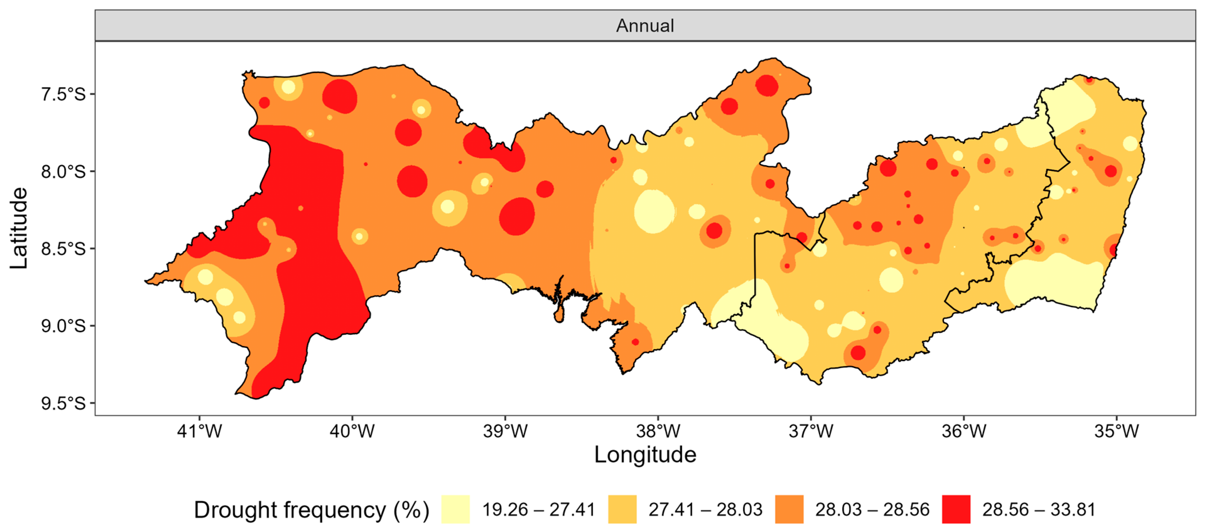
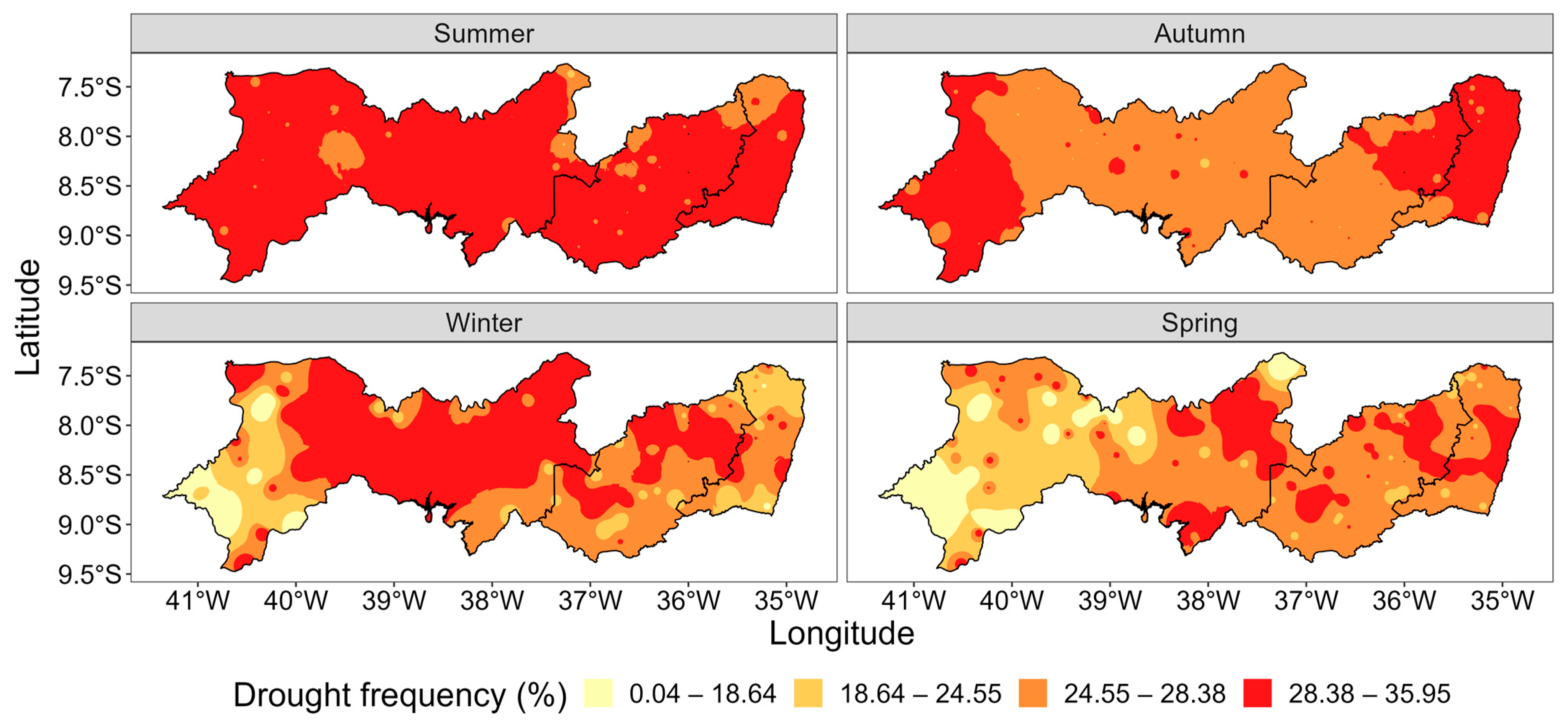
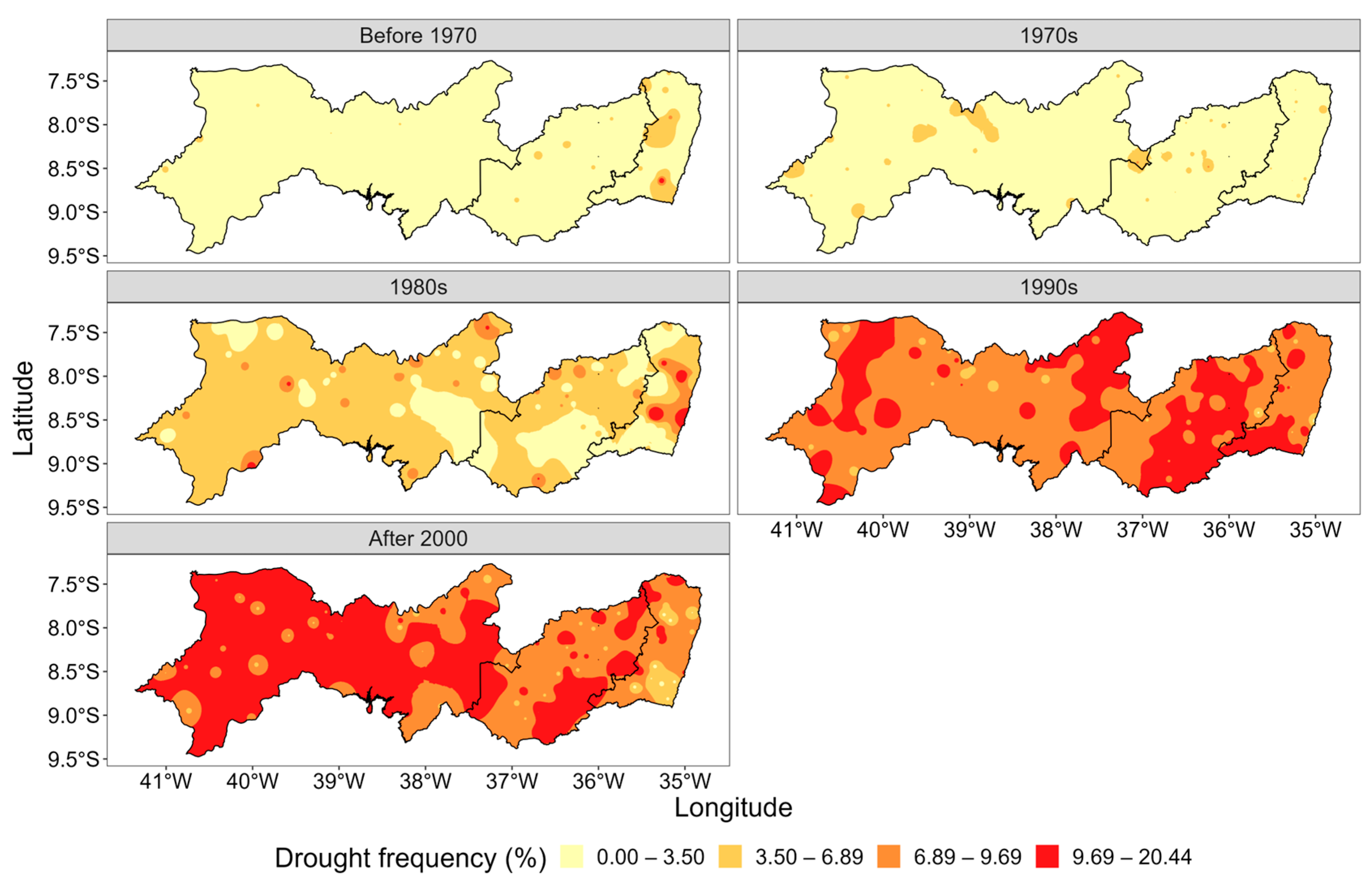
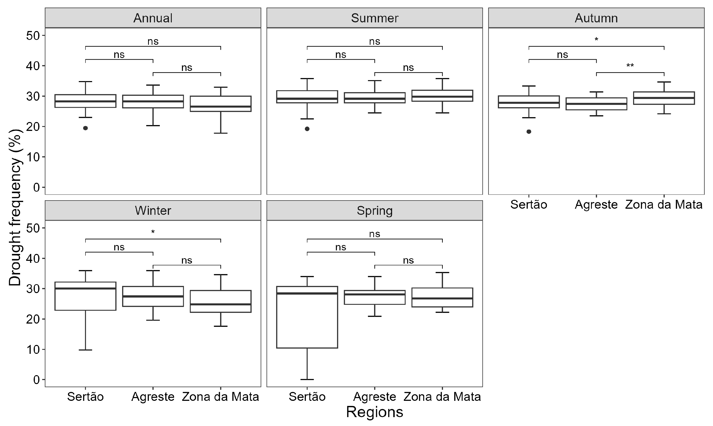
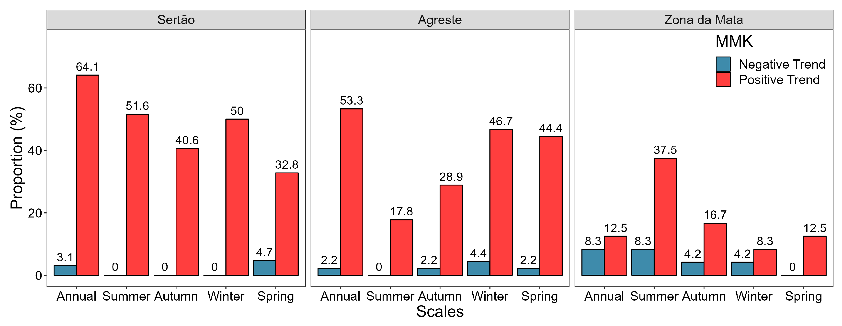
3.1. Drought Frequency

The spatial distribution of the annual drought frequency in the state of Pernambuco during the analyzed period (1962–2012) is shown in Figure 2. The observed frequency values, obtained via Equation (7), were interpolated using the IDW method. The range between the maximum and minimum values of drought frequency has been divided into four intervals (as indicated in the legend), defined according to the k-means clustering method [90]. The result shows that the highest values of drought frequency are found in the western part of the Sertão of Pernambuco, which is a region of the state known as the most frequently affected by droughts [52]. On average, the state of Pernambuco presented a frequency of 28%, with values between 19.26% and 33.81%. Averaging by region, the results revealed a mean frequency of 28.50% (the highest percentage) in Sertão. In the Agreste region, the average drought percentage was 27.80%. Zona da Mata, on the other hand, was the region with the lowest drought frequency. Although its average percentage of drought (27.72%) is very close to that of the Agreste.

The drought frequency distributions on a seasonal scale (obtained from the SPI-3 values) are presented in Figure 3, for summer (December–February), autumn (March–May), winter (June–August), and spring (September–November). Here, the k-means clustering method [90] was used again to divide the range between the maximum and minimum values of the drought frequency into four intervals. During the summer, Pernambuco experienced high drought frequencies in practically its entire territory, with percentages that varied between 24.55% and 35.95%, achieving an average of 29.93%. During autumn, higher frequencies were observed in the extremes of Pernambuco (west of the Sertão, east of the Agreste, and in almost the entire Zona da Mata), and the percentages varied between 24.18% and 34.64%, with an average of 29.52%; while, during the winter, there was a higher frequency of droughts in the central region of the Sertão, with variation between 17.64% and 34.64% and a mean value of 25.29%. During spring, the frequency of drought varied between 22.22% and 35.29% (with an average of 27.53%), and most of the territory exhibited lower drought frequencies in comparison to the other seasons.

Aiming to investigate the drought frequency by decade, the analyzed period (1962–2012) has been divided into five sub-periods: from 1962 to 1970 (before 1970), 1970s, 1980s, 1990s, and from 2000 to 2012 (after 2000). The spatial distribution of drought frequency on an annual scale for each sub-period is shown in Figure 4. The results indicate differences between decades, with a clear increase in the drought frequency over the periods considered. In the period between 1962 and 1970 (before 1970), Pernambuco state exhibited a uniform distribution with low drought occurrence (<3.50%) in almost all of its entirety, except for Zona da Mata, which presented areas with frequency within the range between 3.50% and 6.89% and one point (to the south) between 6.89% and 20.44%. In the 1970s, there was also low drought occurrence in most of the state, with some small areas in Sertão and Agreste regions presenting an increase in frequency from values < 3.50% to values within the range between 3.50% and 6.89% and a decrease in Zona da Mata when compared with the sub-period before 1970. Contrasts in drought frequency distribution became more evident in the 1980s, although the prevailing statewide frequency values varied between 3.5 and 6.89%. In addition, Zona da Mata exhibited in this decade the largest areas with the highest frequency values (between 9.69 and 20.44%). In the 1990s, there was a relevant increase in drought frequency, especially in the west and east of the Sertão, almost all of the Agreste, and in the south of the Zona da Mata. After the year 2000, there was drought with a frequency between 9.69 and 20.44% in almost the entire state of Pernambuco, except in the south of the Zona da Mata region. The results shown in Figure 4 are in agreement with what is stated by Marengo et al. [21], in which the droughts that lasted in Northeastern Brazil until recent years, possibly in the 1990s, a decade that also registered very intense droughts, especially in the years 1993 and 1998.

Statistical differences between Pernambuco regions (Sertão, Agreste, and Zona da Mata) regarding drought frequency have been investigated by applying the Wilcoxon–Mann–Whitney test [91] to the spatial distributions of Figure 2 (annual scale) and Figure 3 (seasonal scale). Figure 5 depicts the distribution of drought frequency values and the results of the applied test. The median drought frequency values are concentrated around 30% for both. On an annual scale, one observes statistical differences between Sertão and Zona da Mata to the level of 5% ($pv<0.05$) for autumn and winter and between Agreste and Zona da Mata to the level of 1% ($pv<0.01$) for autumn. There were no significant statistical differences on a seasonal scale during the summer and spring between all the regions, as well as on the annual scale.

In order to investigate trends in drought frequency for the 133 weather stations, this drought indicator was calculated for each year via Equation (7) on annual and seasonal scales. The results of the modified Mann–Kendall test for each time series of drought frequency are illustrated in Figure 6, where the symbols indicate the geographic location of the weather stations. The red triangles represent significant ($pv<0.05$) positive trends, while the blue triangles represent negative trends. Gray circles refer to non-significant trends.

The proportion of weather stations with significant trends, calculated by region (Sertão, Agreste, and Zona da Mata) on annual and seasonal scales, is illustrated in Figure 7, where red bars represent the percentage of positive significant trends and blue bars represent negative significant trends. The results show that Sertão was the region with the highest proportion of stations, with positive trends for all scales. The fact that this region is getting drier has also been noted by Assis et al. [92] and Silva and Azevedo [93].

The spatial distribution of trend magnitude (Sen’s slope values interpolated across Pernambuco state) in drought frequency on annual (SPI-12) and seasonal (SPI-3) scales is presented in Figure 8. On an annual scale, the trend magnitude showed to be more expressive in western Pernambuco, a region heavily impacted by drought events [52], and eastern Agreste. On a seasonal scale, one observes the highest values of trend magnitude in northwest Pernambuco during summer and autumn and in the Agreste region (center and north) during the spring and winter. In addition, the trend’s magnitudes showed to be more expressive in the eastern part of the Sertão during winter.

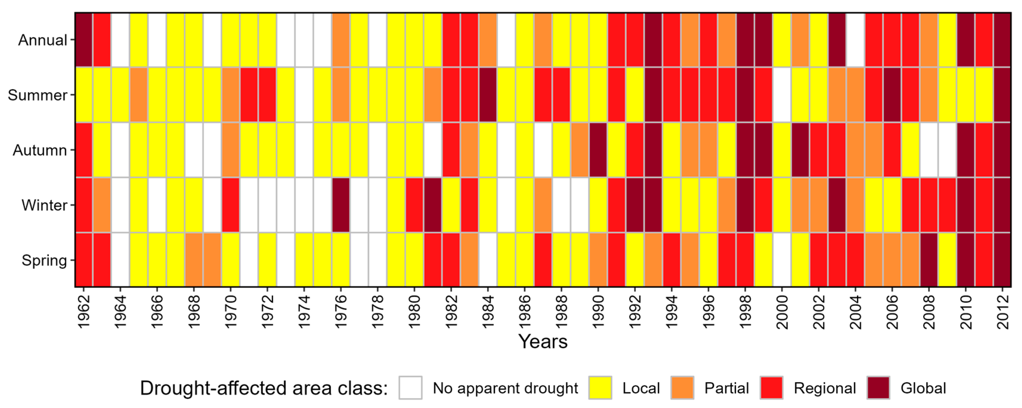
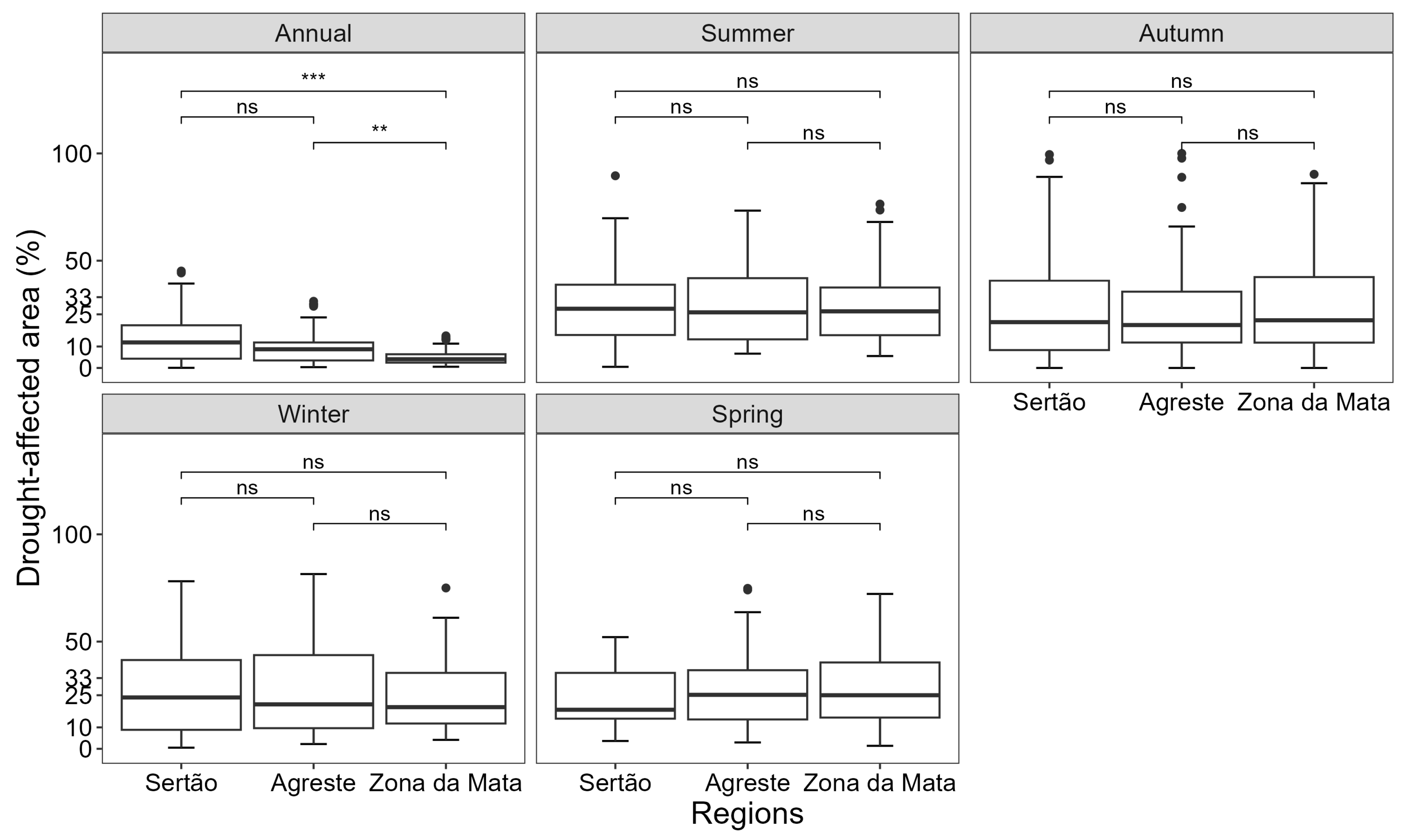
3.2. Drought-Affected Area

Results obtained for the drought-affected area (station proportion, in percentage) on an annual (SPI-12) and seasonal (SPI-3) scale are presented in Figure 9 according to the coverage area class (no apparent drought, local, partial, regional, and global). Global coverage of droughts at all scales has become more frequent since 1990, a period in which the Brazilian Northeast was severely impacted by droughts [35]. On an annual scale, the drought-affected area varied from 1.38% (no apparent drought) to 90.10% (global), with an average of 28.50% (partial regional drought). On a seasonal scale, the drought-affected area values range from 7.52% (no apparent drought) to 67.40% (global drought) in summer, 0% (no apparent drought) to 96% (global drought) in autumn, 2.51% (no apparent drought) to 76.20% (global drought) in winter, and 4.01% (no apparent drought) to 57.60% (global drought) in spring, with an average of 29.40% (partial regional drought), 28% (partial regional drought), 26.90% (partial regional drought), and 25.5% (partial regional drought), respectively.

The highest percentages of areas affected by drought occurred in 1993 (during autumn and on an annual scale), 2012 (during winter and summer), and 2008 (during spring). During the year 1993 (when the affected area reached its maximum values), one of the most severe droughts ever experienced by the Brazilian Northeast occurred, which, according to Rao [94] and Cunha [50], was caused by an atypical El Niño event. The year 1998 was part of the period of one of the worst droughts faced by the Brazilian Northeast [25]. There are also records of months of severe and extreme droughts that impacted the region in 2008 [50,95]. The peaks in the drought-affected area observed in 2012 are related to the migration of the Intertropical Convergence Zone (ITCZ) to the north, followed by an El Niño event [50].

Aiming to investigate possible trends around the values of the drought-affected area on the annual (SPI-12) and seasonal (SPI-3) scales, the MMK test was performed as well as Sen’s slope to extract their magnitudes. The results showed (

Table 3. Modified Mann–Kendall test of trend and Sen’s slope for the drought-affected area on annual (SPI-12) and seasonal (SPI-3) scales. The symbol “****” correspond to the significant level of 0.01%.

Scales	Modified Mann–Kendall Test
	$\mathit{Z}$	$\mathit{p}\mathit{v}$	Sen Slope	Result
Annual	8.90	5.66 × 10−19 (****)	0.67	Positive Trend
Summer	6.15	7.61 × 10−10 (****)	0.36	Positive Trend
Autumn	5.47	4.45 × 10−8 (****)	0.54	Positive Trend
Spring	5.76	8.21 × 10−9 (****)	0.41	Positive Trend
Winter	9.00	2.17 × 10−19 (****)	0.58	Positive Trend

) a positive (Z > 0) significant ($pv<0.0001$) trend for both scales, and, according to the Sen’s slope (0.67), the Pernambuco state experienced an increase of 0.67% per year in the spatial coverage of drought-affected areas on an annual scale, totaling an increase of 34.17% for the analyzed period (1962–2012). On a seasonal scale, the trend analysis revealed an increase of 0.36%, 0.54%, 0.41%, and 0.58% for the analyzed period during the summer, autumn, winter, and spring, respectively. A positive trend in drought-affected areas has been reported in South America between 1905 and 2005 [96].

In order to distinguish between the regions of Pernambuco in terms of drought-affected areas, the Wilcoxon–Mann–Whitney test [91] has been applied, and the results are exhibited in Figure 10. It is possible to observe a reduction (from local drought to no apparent drought class) in the drought-affected area towards the coast (west to east), with the Zona da Mata differing statistically from the Sertão and Agreste at a significance level of 0.1% and 1%, respectively, on an annual scale. As for the seasonal scale, no statistical difference was observed between the regions. Their median drought-affected area values are concentrated in the partial regional drought (summer and spring) and local drought (autumn and winter) classes.

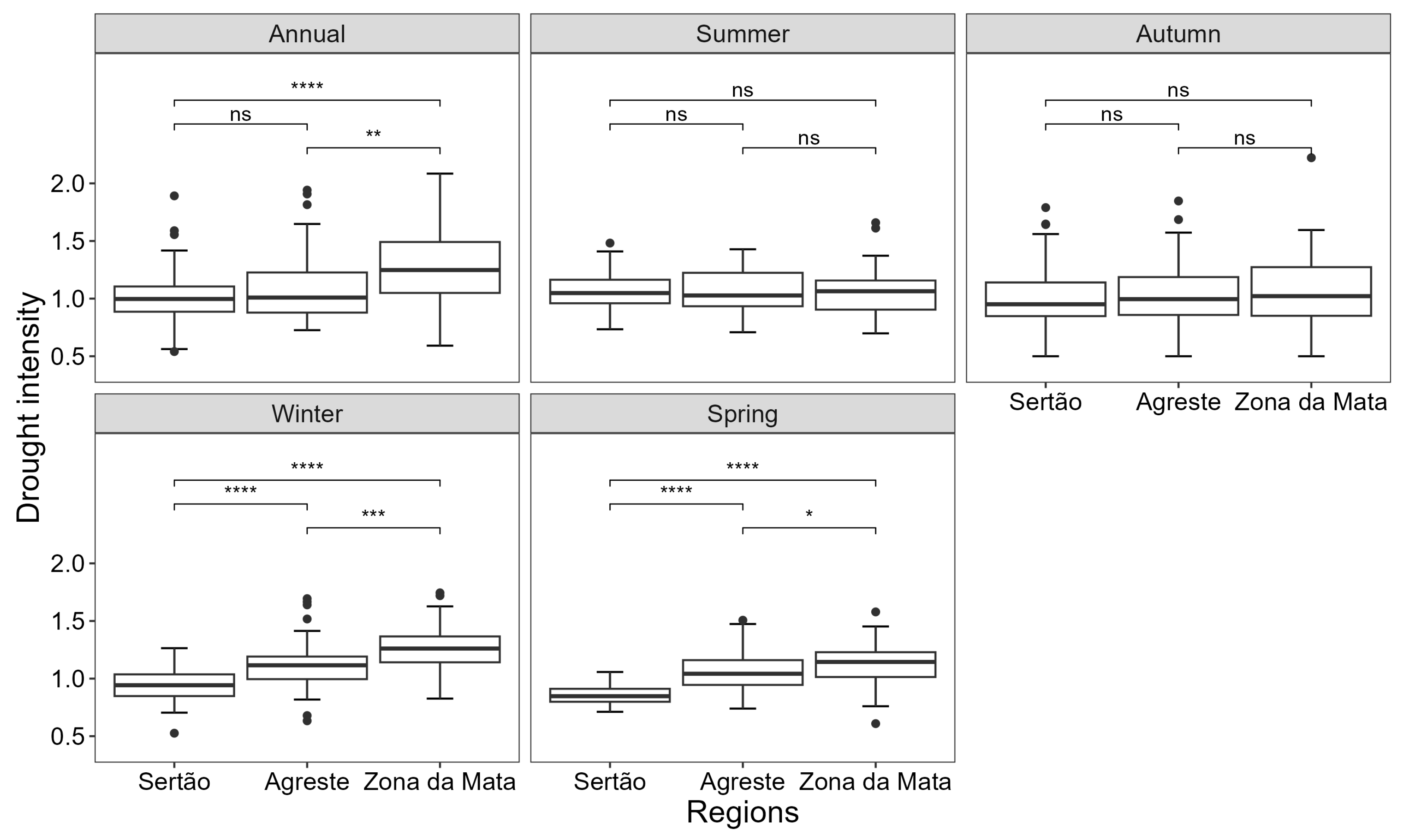
3.3. Drought Intensity

The results of the drought intensity (calculated by Equation (9)) between 1962 and 2012 on annual and seasonal scales are presented in Figure 11. On an annual scale, drought intensity varied between 0.72 (light drought) and 1.93 (heavy drought), with an average of 1.09 (moderate drought). Droughts above moderate were identified in most of the years analyzed. Heavy droughts were observed in 1993, 1998, and 2012. On the seasonal scale, drought intensity values vary from 0.83 (light drought) to 1.39 (moderate drought) in summer, 0.50 (light drought) to 1.78 (heavy drought) in autumn, 0.83 (light drought) to 1.44 (moderate drought) in winter, and 0.79 (light drought) to 1.25 (moderate drought) in spring, with average values equal to 1.08 (moderate drought), 1.05 (moderate drought), 1.06 (moderate drought), and 0.97 (light drought), respectively. It is worth noting that although summer had the highest average drought intensity, it was in autumn that three years (1993, 1998, and 2012) with heavy drought were observed, as well as on an annual scale. These were years in which the Brazilian Northeast experienced severe droughts, leading to a loss of agricultural production and a state of emergency in several places [26].

As can be seen in Figure 11, droughts (at least light droughts) were identified in all the years and at all the scales considered, thus reflecting the normalization of drought in the state of Pernambuco.

Table 4. Modified Mann–Kendall test of trend and Sen’s slope for the drought intensity on annual (SPI-12) and seasonal (SPI-3) scales. The symbols “**”, “***”, and “****” correspond to the significant levels of 1%, 0.1%, and 0.01%, respectively.

Scales	Modified Mann–Kendall Test
	$\mathit{Z}$	$\mathit{p}\mathit{v}$	Sen Slope	Result
Annual	3.38	7.17 × 10−4 (***)	3.35 × 10−3	Positive Trend
Summer	4.75	1.99 × 10−6 (****)	2.81 × 10−3	Positive Trend
Autumn	3.51	4.49 × 10−4 (***)	3.71 × 10−3	Positive Trend
Spring	3.16	1.59 × 10−3 (**)	2.26 × 10−3	Positive Trend
Winter	3.12	1.79 × 10−3 (**)	2.18 × 10−3	Positive Trend

shows a significant positive trend in drought intensity at all the scales analyzed. The magnitude of these trends (Sen’s slope) is strongest in autumn (3.71 × 10⁻³), followed by annual (3.35 × 10⁻³), summer (2.81 × 10⁻³), spring (2.26 × 10⁻³), and winter (2.18 × 10⁻³).

We also evaluated statistical differences between Pernambuco regions (Sertão, Agreste, and Zona da Mata) regarding drought intensity on annual and seasonal scales. For this, the Wilcoxon–Mann–Whitney test [91] has been applied, and the results are exhibited in Figure 12, together with the distribution of drought intensity values. On the annual scale, it is possible to observe an increase (from 1 to 1.25) in the median values of drought intensity towards the coast (west to east) and that the Zona da Mata statistically differs from the Sertão and Agreste. On the seasonal scale, summer and autumn showed no significant difference between the regions, and their median values are concentrated around 1.0 (moderate drought). On the other hand, there is a significant difference between the three regions in spring and winter. In both spring and winter, there was an increase from west to east in the median drought intensity values, from 0.85 (light drought) to 1.14 (moderate drought) in spring and 0.94 (light drought) to 1.26 (moderate drought) in winter. The distinction between these regions was also observed when evaluating the persistence, disorder, and structural organization of dry/wet conditions [97,98].

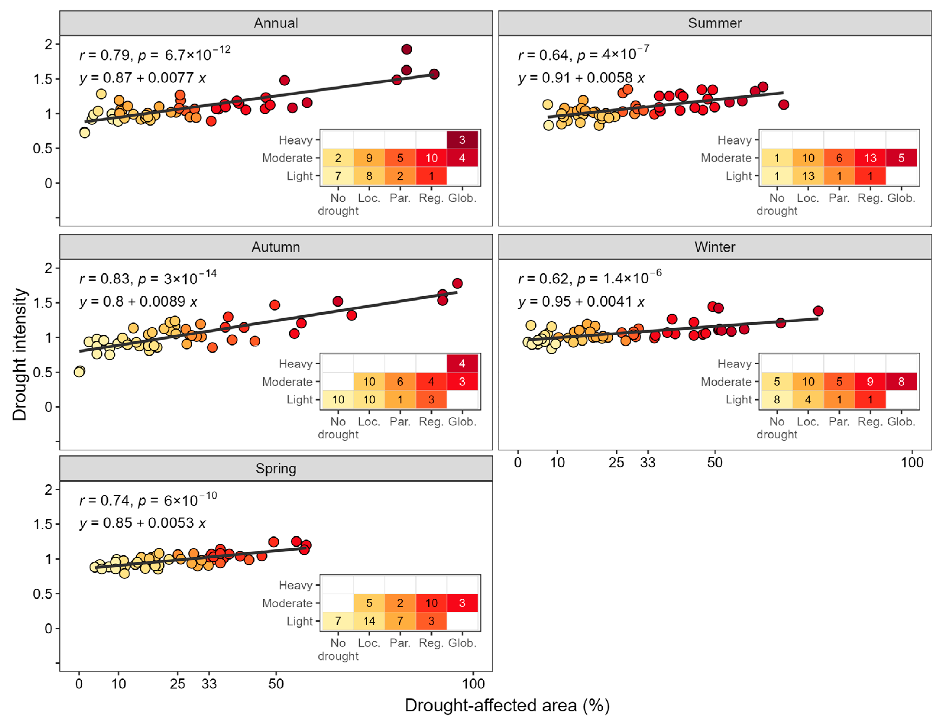
3.4. Relationship between Drought Area and Intensity

In order to identify which years showed high (low) covered drought-affected areas and high (low) drought intensity over the period analyzed (1962–2012), we constructed a graph of the temporal evolution of these two drought characteristics on annual (SPI-12) and seasonal (SPI-3) scales, as shown in Figure 13. A priori, we know from the MMK test and Sen’s slope (Table 3 and Table 4) that both drought characteristics showed a significant positive trend on all the scales analyzed, with higher magnitude values (Sen‘s slope) observed at the annual and autumn scales for drought-affected area and drought intensity, respectively. The years with the highest values (global drought and heavy drought classes) for the extent and intensity of the drought were also observed on these scales, specifically in 1993, 1998, 2010 (only autumn), and 2012. Silva et al. [99] found that 1993 and 1998 were classified as very dry and 2012 as extremely dry. The year 2010, on the other hand, was influenced by a weak El Nino, with negative precipitation anomalies in relation to the average [100]. The other scales, summer, spring, and winter, show drought-affected area values that do not reach the global drought class and drought intensity values that do not exceed the moderate drought class.

The relationship between drought-affected areas and drought intensity on annual (SPI-12) and seasonal (SPI-3) scales was investigated. The result is shown in Figure 14, together with the number of years (heatmap within facets) in which a specific drought-affected area class (no apparent, local—Loc., partial regional—Par., regional—Reg., or global—Glob. droughts) and the drought intensity (light, moderate, severe, and extreme droughts) were observed. It can be seen that there is a significant positive correlation (r) between the extent and intensity of drought at all the scales considered, with values equal to 0.79 (annual), 0.64 (summer), 0.83 (autumn), 0.62 (winter), and 0.74 (spring). According to Hinkle et al. [101], the correlations observed at the annual, autumn, and spring scales are considered strong, while the correlations observed at the summer and winter scales are considered moderate. This positive correlation means that the larger the drought area, the higher the drought intensity.

Autumn had the highest correlation (0.83) and the highest number of years (1983, 1993, 1998, and 2012) in which a global drought of heavy intensity was observed. Regoto et al. [102] analyzed precipitation in Brazil between 1961 and 2018 and identified a statistically significant and robust decrease in precipitation in the Northeast region. Furthermore, during the autumn and summer seasons, Northeastern precipitation showed a reduction, leading to a drier climate and longer periods of drought. Brito et al. [52] observed that the drought-affected area in recent years (1981–2012) has increased in the Brazilian semiarid region, of which the state of Pernambuco is part. Similar behavior regarding the relationship between drought extension and intensity was also observed by Yan et al. [61] in Yunnan Province, China. It should be noted that the number of affected stations was used as a proxy for the drought area. Although this number is high and the stations are rather well distributed across the study area, some regions, such as the southeastern part of Sertao, have fewer stations. This could lead to some uncertainties in the presented results as well as in their spatial interpolations. Future work will include a high-resolution gridded climate dataset.

4. Conclusions

This study investigated the spatiotemporal variability of three drought characteristic parameters (frequency, affected area, and intensity) in Pernambuco, Brazil, during the period 1962–2012, using SPI 3 and SPI 12, which describe drought conditions on a seasonal and annual scale, respectively. Based on the results, the following conclusions can be drawn:

• The frequency of annual droughts in the state of Pernambuco has become more frequent since the 1990s, with summer having the greatest coverage, followed by winter, autumn, and spring. In addition, it was observed that the annual drought frequency values did not differ statistically between the Sertão, Agreste, and Zona da Mata regions, as well as in summer and spring. This shows uniformity in the increased frequency of drought throughout the state. It is worth noting that the Sertão was the region with the highest proportion of stations with a positive trend for all scales, followed by the Agreste and Zona da Mata. The highest values of magnitude (Sen‘s slope) of the annual drought frequency were observed in the west of the Sertão and the east of the Agreste. On a seasonal scale, the frequency of drought increased more rapidly in the northwest of Pernambuco during the summer and autumn; in the spring to the east of Agreste; and in the winter to the east of Sertão and the center of Agreste.
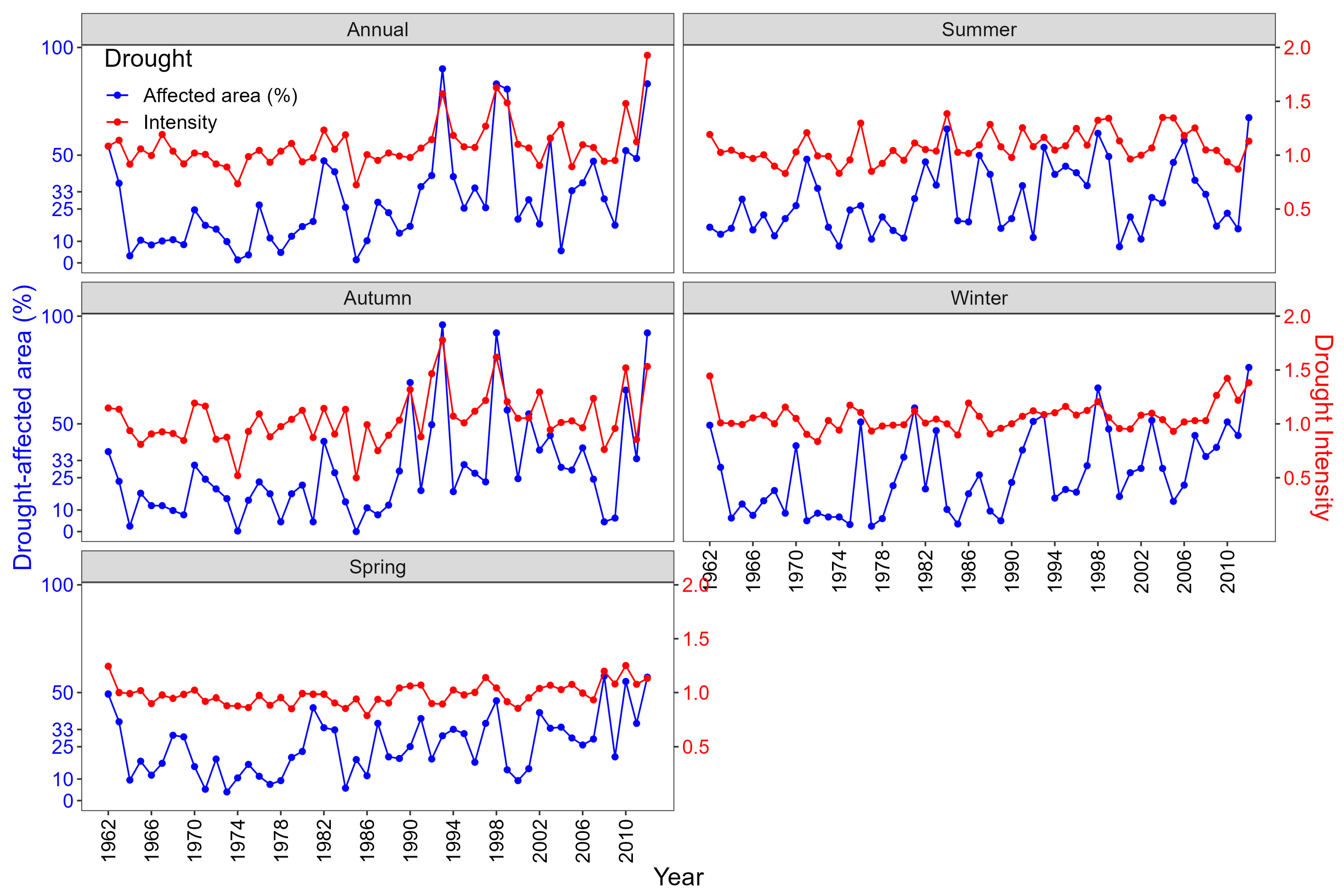
• A significant annual and seasonal upward trend was observed in the coverage and intensity of drought in the state of Pernambuco. The extent and intensity became even more prominent from the 1990s onwards, as observed in the frequency of droughts. This more widespread and intense drought occurred particularly in the years 1993, 1998, 2010, and 2012. These years are often cited in the literature as the years in which the greatest droughts occurred.
• The relationship between drought area and intensity revealed a linear trend between these characteristics, showing high values of positive correlation between the drought extent and intensity across all time scales considered, indicating that the larger the area affected by drought, the higher the intensity will be.

It became clear that over the years (from 1962 to 2012), the state of Pernambuco experienced more frequent, spatially extensive, and intense drought events. The results provide useful information for the development of public policies focused on water resource management throughout the state and the mitigation of the effects of drought on the state‘s population. This approach employed here can be extended to current days and expanded to the Northeast region of Brazil, which is vulnerable to dry events.

References

- Venancio, L.P.; Filgueiras, R.; Mantovani, E.C.; Amaral, C.H.; Cunha, F.F.; Santos Silva, F.C.; Althoff, D.; Santos, R.A.; Cavatte, P.C. Impact of Drought Associated with High Temperatures on Coffea Canephora Plantations: A Case Study in Espírito Santo State, Brazil. Sci. Rep. 2020, 10, 19719. [Google Scholar] [CrossRef] [PubMed]
- Wilhite, D.A. Chapter 1 Drought as a Natural Hazard: Concepts and Definitions. In Drought Mitigation Center Faculty Publications; Routledge: London, UK, 2000; pp. 3–18. [Google Scholar]
- Uwimbabazi, J.; Jing, Y.; Iyakaremye, V.; Ullah, I.; Ayugi, B. Observed Changes in Meteorological Drought Events during 1981–2020 over Rwanda, East Africa. Sustainability 2022, 14, 1519. [Google Scholar] [CrossRef]
- Douris, J.; Kim, G. Atlas of Mortality and Economic Losses from Weather, Climate and Water Extremes (1970–2019); World Meteorological Organization (WMO): Geneva, Switzerland, 2021. [Google Scholar]
- Sena, A.; Barcellos, C.; Freitas, C.; Corvalan, C. Managing the Health Impacts of Drought in Brazil. Int. J. Environ. Res. Public Health 2014, 11, 10737–10751. [Google Scholar] [CrossRef] [PubMed]
- Mekuria, T. The Effects of Flooding and Drought on Clean Water Accesibility in Ethiopia. Hydraul. Eng. Repos. Karlsr. Ger. 2022, 1, 18–21. [Google Scholar]
- Nasir, M.W.; Toth, Z. Effect of Drought Stress on Potato Production: A Review. Agronomy 2022, 12, 635. [Google Scholar] [CrossRef]
- Hanigan, I.C.; Chaston, T.B. Climate Change, Drought and Rural Suicide in New South Wales, Australia: Future Impact Scenario Projections to 2099. Int. J. Environ. Res. Public Health 2022, 19, 7855. [Google Scholar] [CrossRef] [PubMed]
- Atwoli, L.; Muhia, J.; Merali, Z. Mental Health and Climate Change in Africa. BJPsych. Int. 2022, 19, 86–89. [Google Scholar] [CrossRef]
- Contreras, D.; Voets, A.; Junghardt, J.; Bhamidipati, S.; Contreras, S. The Drivers of Child Mortality During the 2012–2016 Drought in La Guajira, Colombia. Int. J. Disaster Risk Sci. 2020, 11, 87–104. [Google Scholar] [CrossRef]
- Epstein, A.; Bendavid, E.; Nash, D.; Charlebois, E.D.; Weiser, S.D. Drought and Intimate Partner Violence towards Women in 19 Countries in Sub-Saharan Africa during 2011–2018: A Population-Based Study. PLoS Med. 2020, 17, e1003064. [Google Scholar] [CrossRef]
- Zhang, Q.; Yu, H.; Sun, P.; Singh, V.P.; Shi, P. Multisource Data Based Agricultural Drought Monitoring and Agricultural Loss in China. Glob. Planet. Chang. 2019, 172, 298–306. [Google Scholar] [CrossRef]
- Wilhite, D.A.; Sivakumar, M.V.K.; Pulwarty, R. Managing Drought Risk in a Changing Climate: The Role of National Drought Policy. Weather Clim. Extrem. 2014, 3, 4–13. [Google Scholar] [CrossRef]
- Jha, S.; Srivastava, R. Impact of Drought on Vegetation Carbon Storage in Arid and Semi-Arid Regions. Remote Sens. Appl. 2018, 11, 22–29. [Google Scholar] [CrossRef]
- Ntali, Y.M.; Lyimo, J.G. Community Livelihood Vulnerability to Drought in Semi-Arid Areas of Northern Cameroon. Discov. Sustain. 2022, 3, 22. [Google Scholar] [CrossRef]
- Wilhite, D.A.; Glantz, M.H. Understanding: The Drought Phenomenon: The Role of Definitions. Water Int. 1985, 10, 111–120. [Google Scholar] [CrossRef]
- Feng, G.; Chen, Y.; Mansaray, L.R.; Xu, H.; Shi, A.; Chen, Y. Propagation of Meteorological Drought to Agricultural and Hydrological Droughts in the Tropical Lancang–Mekong River Basin. Remote Sens. 2023, 15, 5678. [Google Scholar] [CrossRef]
- Panu, U.S.; Sharma, T.C. Challenges in Drought Research: Some Perspectives and Future Directions. Hydrol. Sci. J. 2002, 47, S19–S30. [Google Scholar] [CrossRef]
- Awchi, T.A.; Kalyana, M.M. Meteorological Drought Analysis in Northern Iraq Using SPI and GIS. Sustain. Water Resour. Manag. 2017, 3, 451–463. [Google Scholar] [CrossRef]
- Van Loon, A.F. Hydrological Drought Explained. WIREs Water 2015, 2, 359–392. [Google Scholar] [CrossRef]
- Marengo, J.A.; Alves, L.M.; Alvala, R.C.S.; Cunha, A.P.; Brito, S.; Moraes, O.L.L. Climatic Characteristics of the 2010–2016 Drought in the Semiarid Northeast Brazil Region. Acad. Bras. Cienc. 2018, 90, 1973–1985. [Google Scholar] [CrossRef]
- Marengo, J.A.; Cunha, A.P.; Soares, W.R.; Torres, R.R.; Alves, L.M.; Barros Brito, S.S.; Cuartas, L.A.; Leal, K.; Ribeiro Neto, G.; Alvalá, R.C.S.; et al. Increase Risk of Drought in the Semiarid Lands of Northeast Brazil Due to Regional Warming above 4 °C. In Climate Change Risks in Brazil; Springer International Publishing: Cham, Switzerland, 2019; pp. 181–200. [Google Scholar]
- Silvia, V.M.d.A.; Patício, M.d.C.M.; Ribeiro, V.H.; Medeiros, R.M. O Desastre Seca No Nordeste Brasileiro. Polêm! Ca 2013, 12, 284–293. [Google Scholar] [CrossRef]
- Utida, G.; Cruz, F.W.; Etourneau, J.; Bouloubassi, I.; Schefuß, E.; Vuille, M.; Novello, V.F.; Prado, L.F.; Sifeddine, A.; Klein, V.; et al. Tropical South Atlantic Influence on Northeastern Brazil Precipitation and ITCZ Displacement during the Past 2300 Years. Sci. Rep. 2019, 9, 1698. [Google Scholar] [CrossRef] [PubMed]
- Marengo, J.A.; Galdos, M.V.; Challinor, A.; Cunha, A.P.; Marin, F.R.; Vianna, M.d.S.; Alvala, R.C.S.; Alves, L.M.; Moraes, O.L.; Bender, F. Drought in Northeast Brazil: A Review of Agricultural and Policy Adaptation Options for Food Security. Clim. Resil. Sustain. 2022, 1, e17. [Google Scholar] [CrossRef]
- Marengo, J.A.; Torres, R.R.; Alves, L.M. Drought in Northeast Brazil—Past, Present, and Future. Theor. Appl. Clim. 2017, 129, 1189–1200. [Google Scholar] [CrossRef]
- Mao, Y.; Zou, Y.; Alves, L.M.; Macau, E.E.N.; Taschetto, A.S.; Santoso, A.; Kurths, J. Phase Coherence between Surrounding Oceans Enhances Precipitation Shortages in Northeast Brazil. Geophys. Res. Lett. 2022, 49, e2021GL097647. [Google Scholar] [CrossRef]
- Dikici, M. Drought Analysis with Different Indices for the Asi Basin (Turkey). Sci. Rep. 2020, 10, 20739. [Google Scholar] [CrossRef] [PubMed]
- Tsakiris, G.; Vangelis, H. Establishing a Drought Index Incorporating Evapotranspiration. Eur. Water 2005, 9, 3–11. [Google Scholar]
- Vicente-Serrano, S.M.; Beguería, S.; López-Moreno, J.I. A Multiscalar Drought Index Sensitive to Global Warming: The Standardized Precipitation Evapotranspiration Index. J. Clim. 2010, 23, 1696–1718. [Google Scholar] [CrossRef]
- Svoboda, M.D.; Fuchs, B.A. Handbook of Drought Indicators and Indices; World Meteorological Organization: Geneva, Switzerland, 2016; Volume 2, ISBN 9263111731. [Google Scholar]
- Van-Rooy, M.P. A Rainfall Anomally Index Independent of Time and Space, Notos. Weather Bur. S. Afr. 1965, 14, 43–48. [Google Scholar]
- Wu, H.; Hayes, M.J.; Weiss, A.; Hu, Q. An Evaluation of the Standardized Precipitation Index, the China-Z Index and the Statistical Z-Score. Int. J. Climatol. 2001, 21, 745–758. [Google Scholar] [CrossRef]
- Katz, R.W.; Glantz, M.H. Anatomy of a Rainfall Index. Mon. Weather Rev. 1986, 114, 764–771. [Google Scholar] [CrossRef]
- Kraus, E.B. Subtropical Droughts and Cross-Equatorial Energy Transports. Mon. Weather Rev. 1977, 105, 1009–1018. [Google Scholar] [CrossRef]
- Bhalme, H.N.; Mooley, D.A. Large-Scale Droughts/Floods and Monsoon Circulation. Mon. Weather Rev. 1980, 108, 1197–1211. [Google Scholar] [CrossRef]
- Byun, H.-R.; Wilhite, D.A. Objective Quantification of Drought Severity and Duration. J. Clim. 1999, 12, 2747–2756. [Google Scholar] [CrossRef]
- Strommen, N.D.; Motha, R.P. An Operational Early Warning Agricultural Weather System. In Planning for Drought; Routledge: London, UK, 2019; pp. 153–162. [Google Scholar]
- McKee, T.B.; Doesken, N.J.; Kleist, J. The Relationship of Drought Frequency and Duration to Time Scales. In Proceedings of the 8th Conference on Applied Climatology, Anaheim, CA, USA, 17–22 January 1993; Volume 17, pp. 179–183. [Google Scholar]
- Wang, Q.; Zhang, R.; Qi, J.; Zeng, J.; Wu, J.; Shui, W.; Wu, X.; Li, J. An Improved Daily Standardized Precipitation Index Dataset for Mainland China from 1961 to 2018. Sci. Data 2022, 9, 124. [Google Scholar] [CrossRef] [PubMed]
- Jain, V.K.; Pandey, R.P.; Jain, M.K.; Byun, H.-R. Comparison of Drought Indices for Appraisal of Drought Characteristics in the Ken River Basin. Weather Clim. Extrem. 2015, 8, 1–11. [Google Scholar] [CrossRef]
- Wu, H.; Svoboda, M.D.; Hayes, M.J.; Wilhite, D.A.; Wen, F. Appropriate Application of the Standardized Precipitation Index in Arid Locations and Dry Seasons. Int. J. Climatol. 2007, 27, 65–79. [Google Scholar] [CrossRef]
- Güner Bacanli, Ü. Trend Analysis of Precipitation and Drought in the Aegean Region, Turkey. Meteorol. Appl. 2017, 24, 239–249. [Google Scholar] [CrossRef]
- Akhtari, R.; Mahdian, M.H.; Morid, S. Assessment of Spatial Analysis of SPI and EDI Drought Indices in Tehran Province. Iran-Water Resour. Res. 2007, 2, 27–38. [Google Scholar]
- Nwayor, I.J.; Robeson, S.M. Exploring the Relationship between SPI and SPEI in a Warming World. Theor. Appl. Clim. 2024, 155, 2559–2569. [Google Scholar] [CrossRef]
- Brasil Neto, R.M.; Santos, C.A.G.; Silva, J.F.C.B.d.C.; Silva, R.M.; Santos, C.A.C.; Mishra, M. Evaluation of the TRMM Product for Monitoring Drought over Paraíba State, Northeastern Brazil: A Trend Analysis. Sci. Rep. 2021, 11, 1097. [Google Scholar] [CrossRef]
- Souza, A.; Neto, A.; Rossato, L.; Alvalá, R.; Souza, L. Use of SMOS L3 Soil Moisture Data: Validation and Drought Assessment for Pernambuco State, Northeast Brazil. Remote Sens. 2018, 10, 1314. [Google Scholar] [CrossRef]
- Inocêncio, T.d.M.; Ribeiro Neto, A.; Oertel, M.; Meza, F.J.; Scott, C.A. Linking Drought Propagation with Episodes of Climate-Induced Water Insecurity in Pernambuco State—Northeast Brazil. J. Arid. Environ. 2021, 193, 104593. [Google Scholar] [CrossRef]
- Silva, T.R.B.F.; Santos, C.A.C.d.; Silva, D.J.F.; Santos, C.A.G.; da Silva, R.M.; de Brito, J.I.B. Climate Indices-Based Analysis of Rainfall Spatiotemporal Variability in Pernambuco State, Brazil. Water 2022, 14, 2190. [Google Scholar] [CrossRef]
- Cunha, A.P.M.A.; Tomasella, J.; Ribeiro-Neto, G.G.; Brown, M.; Garcia, S.R.; Brito, S.B.; Carvalho, M.A. Changes in the Spatial–Temporal Patterns of Droughts in the Brazilian Northeast. Atmos. Sci. Lett. 2018, 19, e855. [Google Scholar] [CrossRef]
- Costa, M.d.S.; Oliveira-Júnior, J.F.d.; Santos, P.J.d.; Correia Filho, W.L.F.; Gois, G.d.; Blanco, C.J.C.; Teodoro, P.E.; Silva Junior, C.A.d.; Santiago, D.d.B.; Souza, E.d.O.; et al. Rainfall Extremes and Drought in Northeast Brazil and Its Relationship with El Niño–Southern Oscillation. Int. J. Climatol. 2021, 41, E2111–E2135. [Google Scholar] [CrossRef]
- Brito, S.S.B.; Cunha, A.P.M.A.; Cunningham, C.C.; Alvalá, R.C.; Marengo, J.A.; Carvalho, M.A. Frequency, Duration and Severity of Drought in the Semiarid Northeast Brazil Region. Int. J. Climatol. 2018, 38, 517–529. [Google Scholar] [CrossRef]
- Cunha, A.P.M.A.; Zeri, M.; Deusdará Leal, K.; Costa, L.; Cuartas, L.A.; Marengo, J.A.; Tomasella, J.; Vieira, R.M.; Barbosa, A.A.; Cunningham, C.; et al. Extreme Drought Events over Brazil from 2011 to 2019. Atmosphere 2019, 10, 642. [Google Scholar] [CrossRef]
- Bacia Hidrográfica Do Rio Goiana e Sexto Grupo de Bacias Hidrográficas de Pequenos Rios Litorâneos—GL6; Agência CONDEPE/FIDEM: Recife, Brazil, 2005.
- Galvincio, J.D.; Moura, M.S.B. Aspectos Climáticos Da Captação de Água de Chuva No Estado de Pernambuco. Rev. Geogr. 2005, 22, 100–116. [Google Scholar]
- Hayes, M.; Svoboda, M.; Wall, N.; Widhalm, M. The Lincoln Declaration on Drought Indices: Universal Meteorological Drought Index Recommended. Bull. Am. Meteorol. Soc. 2011, 92, 485–488. [Google Scholar] [CrossRef]
- Stagge, J.H.; Tallaksen, L.M.; Gudmundsson, L.; Van Loon, A.F.; Stahl, K. Candidate Distributions for Climatological Drought Indices (SPI and SPEI). Int. J. Climatol. 2015, 35, 4027–4040. [Google Scholar] [CrossRef]
- Svensson, C.; Hannaford, J.; Prosdocimi, I. Statistical Distributions for Monthly Aggregations of Precipitation and Streamflow in Drought Indicator Applications. Water Resour. Res. 2017, 53, 999–1018. [Google Scholar] [CrossRef]
- Ximenes, P.d.S.M.P.; Silva, A.S.A.; Ashkar, F.; Stosic, T. Ajuste de Distribuições de Probabilidade à Precipitação Mensal No Estado de Pernambuco—Brasil. Res. Soc. Dev. 2020, 9, e4869119894. [Google Scholar] [CrossRef]
- Ximenes, P.d.S.M.P.; Silva, A.S.A.; Ashkar, F.; Stosic, T. Best-Fit Probability Distribution Models for Monthly Rainfall of Northeastern Brazil. Water Sci. Technol. 2021, 84, 1541–1556. [Google Scholar] [CrossRef] [PubMed]
- Yan, Z.; Zhang, Y.; Zhou, Z.; Han, N. The Spatio-Temporal Variability of Droughts Using the Standardized Precipitation Index in Yunnan, China. Nat. Hazards 2017, 88, 1023–1042. [Google Scholar] [CrossRef]
- R Core Team. A Language and Environment for Statistical Computing. R Foundation for Statistical Computing; R Core Team: Vienna, Austria, 2024. [Google Scholar]
- Mann, H.B. Nonparametric Tests Against Trend. Econometrica 1945, 13, 245. [Google Scholar] [CrossRef]
- Kendall, M.G. Rank Correlation Methods; Charles Griffin & Co. Ltd.: London, UK, 1962; p. 160. [Google Scholar]
- Birsan, M.-V.; Dumitrescu, A.; Micu, D.M.; Cheval, S. Changes in Annual Temperature Extremes in the Carpathians since AD 1961. Nat. Hazards 2014, 74, 1899–1910. [Google Scholar] [CrossRef]
- von Storch, H. Misuses of Statistical Analysis in Climate Research. In Analysis of Climate Variability; Springer: Berlin/Heidelberg, Germany, 1995; pp. 11–26. [Google Scholar]
- Mullick, M.d.R.A.; Nur, R.M.; Alam, M.d.J.; Islam, K.M.A. Observed Trends in Temperature and Rainfall in Bangladesh Using Pre-Whitening Approach. Glob. Planet. Chang. 2019, 172, 104–113. [Google Scholar] [CrossRef]
- Bayazit, M.; Önöz, B. To Prewhiten or Not to Prewhiten in Trend Analysis? Hydrol. Sci. J. 2007, 52, 611–624. [Google Scholar] [CrossRef]
- Chowdhury, R.K.; Beecham, S. Australian Rainfall Trends and Their Relation to the Southern Oscillation Index. Hydrol. Process. 2009, 24, 504–514. [Google Scholar] [CrossRef]
- Douglas, E.M.; Vogel, R.M.; Kroll, C.N. Trends in Floods and Low Flows in the United States: Impact of Spatial Correlation. J. Hydrol. 2000, 240, 90–105. [Google Scholar] [CrossRef]
- Yue, S.; Pilon, P.; Phinney, B. Canadian Streamflow Trend Detection: Impacts of Serial and Cross-Correlation. Hydrol. Sci. J. 2003, 48, 51–63. [Google Scholar] [CrossRef]
- Yue, S.; Wang, C. The Mann-Kendall Test Modified by Effective Sample Size to Detect Trend in Serially Correlated Hydrological Series. Water Resour. Manag. 2004, 18, 201–218. [Google Scholar] [CrossRef]
- Bayley, G.V.; Hammersley, J.M. The “Effective” Number of Independent Observations in an Autocorrelated Time Series. Suppl. J. R. Stat. Soc. 1946, 8, 184. [Google Scholar] [CrossRef]
- Salas, J.D.; Delleur, J.W.; Yevjevich, V.; Lane, W.L. Applied Modeling of Hydrologic Time Series; Water Resources Publications: Littleton, CO, USA, 1980. [Google Scholar]
- Swain, S.; Mishra, S.K.; Pandey, A.; Dayal, D. Spatiotemporal Assessment of Precipitation Variability, Seasonality, and Extreme Characteristics over a Himalayan Catchment. Theor. Appl. Clim. 2022, 147, 817–833. [Google Scholar] [CrossRef]
- Araújo, L.S.; Silva, A.S.A.; Menezes, R.S.C.; Stosic, B.; Stosic, T. Analysis of Rainfall Seasonality in Pernambuco, Brazil. Theor. Appl. Clim. 2023, 153, 137–154. [Google Scholar] [CrossRef]
- Stosic, T.; Tošić, M.; Lazić, I.; Silva Araújo, L.; Silva, A.S.A.; Putniković, S.; Djurdjević, V.; Tošić, I.; Stosic, B. Changes in Rainfall Seasonality in Serbia from 1961 to 2020. Theor. Appl. Clim. 2024, 155, 4123–4138. [Google Scholar] [CrossRef]
- Sen, P.K. Estimates of the Regression Coefficient Based on Kendall’s Tau. J. Am. Stat. Assoc. 1968, 63, 1379–1389. [Google Scholar] [CrossRef]
- Patakamuri, S.K.; O’Brien, N. Modified Versions of Mann Kendall and Spearman’s rho Trend Tests. R Package Version 1.6. 2023. Available online: https://CRAN.R-project.org/package=modifiedmk (accessed on 15 November 2023).
- Shepard, D. A Two-Dimensional Interpolation Function for Irregularly-Spaced Data. In Proceedings of the 1968 23rd ACM National Conference, New York, NY, USA, 27–29 August 1968; ACM Press: New York, NY, USA; pp. 517–524. [Google Scholar]
- Silva, A.S.A.; Stosic, B.; Menezes, R.S.C.; Singh, V.P. Comparison of Interpolation Methods for Spatial Distribution of Monthly Precipitation in the State of Pernambuco, Brazil. J. Hydrol. Eng. 2019, 24, 04018068. [Google Scholar] [CrossRef]
- Sobjak, R.; Souza, E.G.; Bazzi, C.L.; Opazo, M.A.U.; Mercante, E.; Aikes Junior, J. Process Improvement of Selecting the Best Interpolator and Its Parameters to Create Thematic Maps. Precis. Agric. 2023, 24, 1461–1496. [Google Scholar] [CrossRef]
- Robinson, T.P.; Metternicht, G. Testing the Performance of Spatial Interpolation Techniques for Mapping Soil Properties. Comput. Electron. Agric. 2006, 50, 97–108. [Google Scholar] [CrossRef]
- Tiwari, S.; Kumar Jha, S.; Sivakumar, B. Reconstruction of Daily Rainfall Data Using the Concepts of Networks: Accounting for Spatial Connections in Neighborhood Selection. J. Hydrol. 2019, 579, 124185. [Google Scholar] [CrossRef]
- Chutsagulprom, N.; Chaisee, K.; Wongsaijai, B.; Inkeaw, P.; Oonariya, C. Spatial Interpolation Methods for Estimating Monthly Rainfall Distribution in Thailand. Theor. Appl. Clim. 2022, 148, 317–328. [Google Scholar] [CrossRef]
- Cressie, N.A.C. Statistics for Spatial Data; John Wiley & Sons, Inc: Hoboken, NJ, USA, 1993; ISBN 9780471002550. [Google Scholar]
- Wikle, C.K.; Zammit-Mangion, A.; Cressie, N. Spatio-Temporal Statistics with R, 1st ed.; Chapman & Hall/CRC: Boca Raton, FL, USA, 2019; Volume 1. [Google Scholar]
- Gräler, B.; Pebesma, E.; Heuvelink, G. Spatio-Temporal Interpolation Using Gstat. R J. 2016, 8, 204–218. [Google Scholar] [CrossRef]
- Pebesma, E.J. Multivariable Geostatistics in S: The Gstat Package. Comput. Geosci. 2004, 30, 683–691. [Google Scholar] [CrossRef]
- Bivand, R.; Ono, H.; Dunlap, R.; Stigler, M. ClassInt: Choose Univariate Class Intervals. R Package Version 0.1–21. 2013. Available online: http://CRAN.R-project.org/package=classInt (accessed on 15 November 2023).
- Mann, H.B.; Whitney, D.R. On a Test of Whether One of Two Random Variables Is Stochastically Larger than the Other. Ann. Math. Stat. 1947, 18, 50–60. [Google Scholar] [CrossRef]
- Assis, J.M.O.; Sobral, M.d.C.M.; Souza, W.M. Análise de Detecção de Variabilidades Climáticas Com Base Na Precipitação Nas Bacias Hidrográficas Do Sertão de Pernambuco. Rev. Bras. Geogr. Fís. 2012, 5, 630–645. [Google Scholar] [CrossRef]
- Silva, F.J.B.C.; Azevedo, J.R.G. Temporal Trend of Drought and Aridity Indices in Semi-Arid Pernambucano to Determine Susceptibility to Desertification. Braz. J. Water Resour. 2020, 25, e32. [Google Scholar] [CrossRef]
- Rao, V.B.; Hada, K.; Herdies, D.L. On the Severe Drought of 1993 in North-east Brazil. Int. J. Climatol. 1995, 15, 697–704. [Google Scholar] [CrossRef]
- Carmo, M.V.N.S.; Lima, C.H.R. Caracterização Espaço-Temporal Das Secas No Nordeste a Partir Da Análise Do Índice SPI. Rev. Bras. Meteorol. 2020, 35, 233–242. [Google Scholar] [CrossRef]
- Wang, Q.; Wu, J.; Lei, T.; He, B.; Wu, Z.; Liu, M.; Mo, X.; Geng, G.; Li, X.; Zhou, H.; et al. Temporal-Spatial Characteristics of Severe Drought Events and Their Impact on Agriculture on a Global Scale. Quat. Int. 2014, 349, 10–21. [Google Scholar] [CrossRef]
- Silva, A.S.A.; Menezes, R.S.C.; Telesca, L.; Stosic, B.; Stosic, T. Fisher Shannon Analysis of Drought/Wetness Episodes along a Rainfall Gradient in Northeast Brazil. Int. J. Climatol. 2021, 41, E2097–E2110. [Google Scholar] [CrossRef]
- Silva, A.S.A.; Filho, M.C.; Menezes, R.S.C.; Stosic, T.; Stosic, B. Trends and Persistence of Dry–Wet Conditions in Northeast Brazil. Atmosphere 2020, 11, 1134. [Google Scholar] [CrossRef]
- Silva, A.R.; Santos, T.S.; Queiroz, D.É.; Gusmão, M.O.; Silva, T.G.F. Variações No Índice de Anomalia de Chuva No Semiárido. J. Environ. Anal. Prog. 2017, 2, 377–384. [Google Scholar] [CrossRef]
- Duarte, C.C.; Nóbrega, R.S.; Coutinho, R.Q. Análise Climatológica e Dos Eventos Extremos de Chuva No Município Do Ipojuca, Pernambuco. Rev. Geogr. (UFPE) 2015, 32, 158–176. [Google Scholar]
- Hinkle, D.E.; Wiersma, W.; Jurs, S.G. Applied Statistics for the Behavioral Sciences; Houghton Mifflin: Boston, MA, USA, 2003; Volume 663. [Google Scholar]
- Regoto, P.; Dereczynski, C.; Chou, S.C.; Bazzanela, A.C. Observed Changes in Air Temperature and Precipitation Extremes over Brazil. Int. J. Climatol. 2021, 41, 5125–5142. [Google Scholar] [CrossRef]