Abstract
East Asia is a region that is highly vulnerable to drought disasters during the spring season, as this period is critical for planting, germinating, and growing staple crops such as wheat, maize, and rice. The climate in East Asia is significantly influenced by three large-scale climate variations: the Pacific Decadal Oscillation (PDO), the El Niño–Southern Oscillation (ENSO), and the Indian Ocean Dipole (IOD) in the Pacific and Indian Oceans. In this study, the spring meteorological drought was quantified using the standardized precipitation evapotranspiration index (SPEI) for March, April, and May. Initially, coupled climate networks were established for two climate variables: sea surface temperature (SST) and SPEI. The directed links from SST to SPEI were determined based on the Granger causality test. These coupled climate networks revealed the associations between climate variations and meteorological droughts, indicating that semi-arid areas are more sensitive to these climate variations. In the spring, PDO and ENSO do not cause extreme wetness or dryness in East Asia, whereas IOD does. The remote impacts of these climate variations on SPEI can be partially explained by atmospheric circulations, where the combined effects of air temperatures, winds, and air pressure fields determine the wet/dry conditions in East Asia.
1. Introduction
A drought is a prevalent and intricate natural phenomenon primarily attributed to a prolonged period of inadequate precipitation, coupled with the compounded effects of elevated evapotranspiration due to climatic factors such as higher temperatures, lower relative humidity, or intense winds [1,2]. The consequences of droughts are devastating; they affect agriculture, water resources, ecosystems, human health, and the economy. In the context of global warming, it is imperative to prioritize attention to the adverse impacts of droughts [1,3,4]. Firstly, global warming may alter global precipitation patterns. As temperatures rise, evaporation rates increase, potentially changing the distribution and amount of rainfall. This can lead to reduced precipitation in certain regions, rendering them more susceptible to drought conditions. Wilhite and Glantz [5] have classified droughts into four types: meteorological, hydrologic, agricultural, and socioeconomic droughts. Meteorological droughts focus on atmospheric conditions, hydrological droughts are concerned with water bodies, agricultural droughts pertain to crop health, and socioeconomic droughts address broader societal and economic impacts [6,7]. In this study, we will examine meteorological droughts, defined as deficiencies in precipitation [8], and serving as precursors to hydrological, agricultural, and socioeconomic droughts.
In the past few decades, many drought indices have been used in studies to measure drought conditions, such as rainfall deciles (RDs) [9], the Palmer drought severity index (PDSI) [10], the standardized precipitation index (SPI) [11], the standardized precipitation evapotranspiration index (SPEI) [12], and the modified version of PDSI [13]. RDs are useful for understanding how current rainfall patterns deviate from normal states and can provide early alerts for potential drought conditions [9]. SPI is a drought index that focuses solely on precipitation data. It calculates the deviation of precipitation from the long-term average for a given timescale, such as monthly or annually [11]. SPI is a dimensionless index that allows for comparisons across different locations and seasons, making it useful for monitoring drought conditions globally. The PDSI is a more comprehensive drought index that considers both water supply and demand. It takes into account precipitation, evaporation, soil moisture, and other factors, providing a quantitative measure of drought severity and duration [10]. SPEI combines the precipitation and potential evapotranspiration data simultaneously to evaluate drought conditions, effectively capturing the balance between water supply (precipitation) and water demand (evapotranspiration) [12,14]. It has been concluded that SPEI is superior to SPI and PDSI because it calculates drought across various timescales, has a simple methodology, and provides robust results [15,16,17]. Moreover, SPEI is supposed to be a much more reasonable approach for analyzing the impacts of climate change on drought occurrence [12,18]. In the past few years, SPEI has been widely applied to study the spatiotemporal characteristics and changing trends of meteorological droughts and dryness/wetness in different areas of the world [19,20,21,22,23]. Mishra and Singh defined meteorological drought as the phenomenon of an atmospheric water deficit due to a precipitation deficit in a period [24]. Ma et al. [25] described a meteorological drought event as having a duration of SPEI for no less than 30 days. Therefore, we have chosen SPEI on a one-month timescale as the meteorological drought index for this study.
East Asia, a densely populated region, relies heavily on agriculture for its social, economic, and cultural prosperity (Figure 1). The northern and northeastern regions of China serve as the primary production areas for wheat and maize, while rice cultivation is widespread in southern China, the Korean Peninsula, and Japan. In 2022, China alone produced a total of 137 million tons of wheat, 276 million tons of maize, and 211 million tons of rice [26]. In Japan, rice production has consistently exceeded 7.5 million tons from 2012 to 2021 [27]. Spring in East Asia is characterized by variable precipitation patterns [28], making it a crucial time for the planting, germination, and growth of these crops. While some areas receive ample rainfall that favors crop germination and growth, others may encounter drought conditions that adversely impact agriculture. During this period, drought can result in insufficient soil moisture, hindering the normal growth and development of crop roots and seedlings. Moreover, wind patterns play a pivotal role in the spring climate of East Asia. The region experiences diverse wind systems, including seasonal monsoons that significantly alter temperature, humidity, and precipitation levels [29]. Due to these factors, East Asia is particularly vulnerable to drought disasters during the spring season, because the moisture transported by the monsoon is less than in the summer [30]. Studies have shown that droughts have a significant impact on crop yields, including maize in Northeast China and maize, rice, soybean, and wheat across China [31,32].
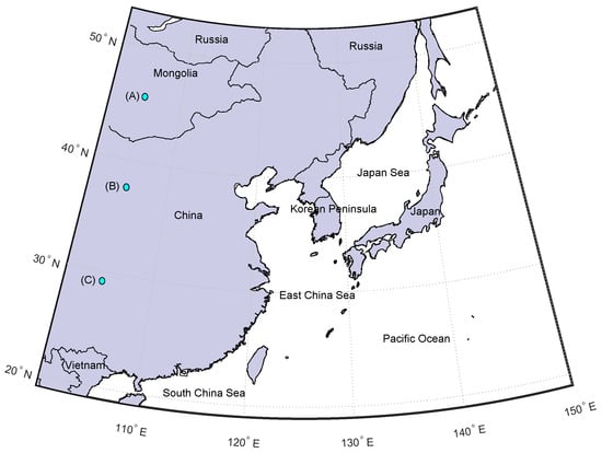
Figure 1.
Location map of the study area (18° N∼55° N, 100° E∼150° E). (A), (B), and (C) are three grid points.
The Pacific Decadal Oscillation (PDO) is a prominent mode of climate variability that operates on a decadal timescale in the Pacific Ocean. This climate variability is characterized by alternating patterns of sea surface temperature (SST) and sea level pressure anomalies, extending from the tropical Pacific to the North Pacific. It has been verified that PDO has exerted significant influence on various aspects of the global climate system, including temperature, precipitation, and extreme events [33,34,35,36,37]. The El Niño–Southern Oscillation (ENSO) is a natural phenomenon that also significantly influences global climate patterns. ENSO is characterized by alternating periods of warm (El Niño) and cold (La Niña) sea surface temperatures in the tropical Pacific Ocean, which trigger complex atmospheric responses and subsequent climate anomalies worldwide. The impact of ENSO on the global climate system has been extensively studied in previous studies, with numerous research articles exploring its diverse effects on temperature, precipitation, and other climatic variables [38,39,40]. ENSO used to be thought of as the primary cause of many episodic droughts around the world. Apart from PDO and ENSO over the Pacific, another large climate mode over the Indian Ocean, IOD, also significantly affects regional climate. IOD refers to the difference in sea surface temperatures between the western and eastern parts of the Indian Ocean. This phenomenon, through its complex sea–air coupling effects, has a significant impact on the climate and environment of the surrounding regions of the Indian Ocean. It can be analogously compared to the ENSO phenomenon in the Pacific Ocean [41,42].
The aim of this study is to delve into the remote effects of large-scale climate variations, such as the PDO, ENSO, and IOD, on meteorological drought during the spring season in East Asia. Although this subject has been extensively researched through traditional correlation analysis, regression analysis, and causality testing in previous studies [43,44,45], this study adopts a novel approach. Specifically, we will first analyze the relationships between climate variations and meteorological drought using coupled climate network analysis. These coupled climate networks will be constructed for two climate variables: the standardized precipitation evapotranspiration index (SPEI) and sea surface temperature (SST). The three climate variations mentioned earlier will be identified through the spatial patterns of SST. The connection between the SPEI node and the SST node will be determined based on the Granger causality test. By observing the spatial patterns of network degrees, we can detect the remote impacts of climate variations on SPEI. Furthermore, we will analyze the mechanisms behind these remote impacts through composite analysis, focusing on atmospheric circulation patterns.
2. Data and Methods
2.1. Data
To calculate the SPEI, we use the CRU TS 4.07 dataset, which is the most complete and updated dataset of gridded precipitation and potential evaporation on a global scale. It has a spatial resolution of 0.5° × 0.5°, ranging from the years 1901 to 2022. The CRU TS 4.07 dataset can be freely accessed from the following website https://crudata.uea.ac.uk/cru/data/hrg/ (accessed on 15 March 2024). In this study, we only analyze the data ranging from 1979 to 2022 covering 44 years.
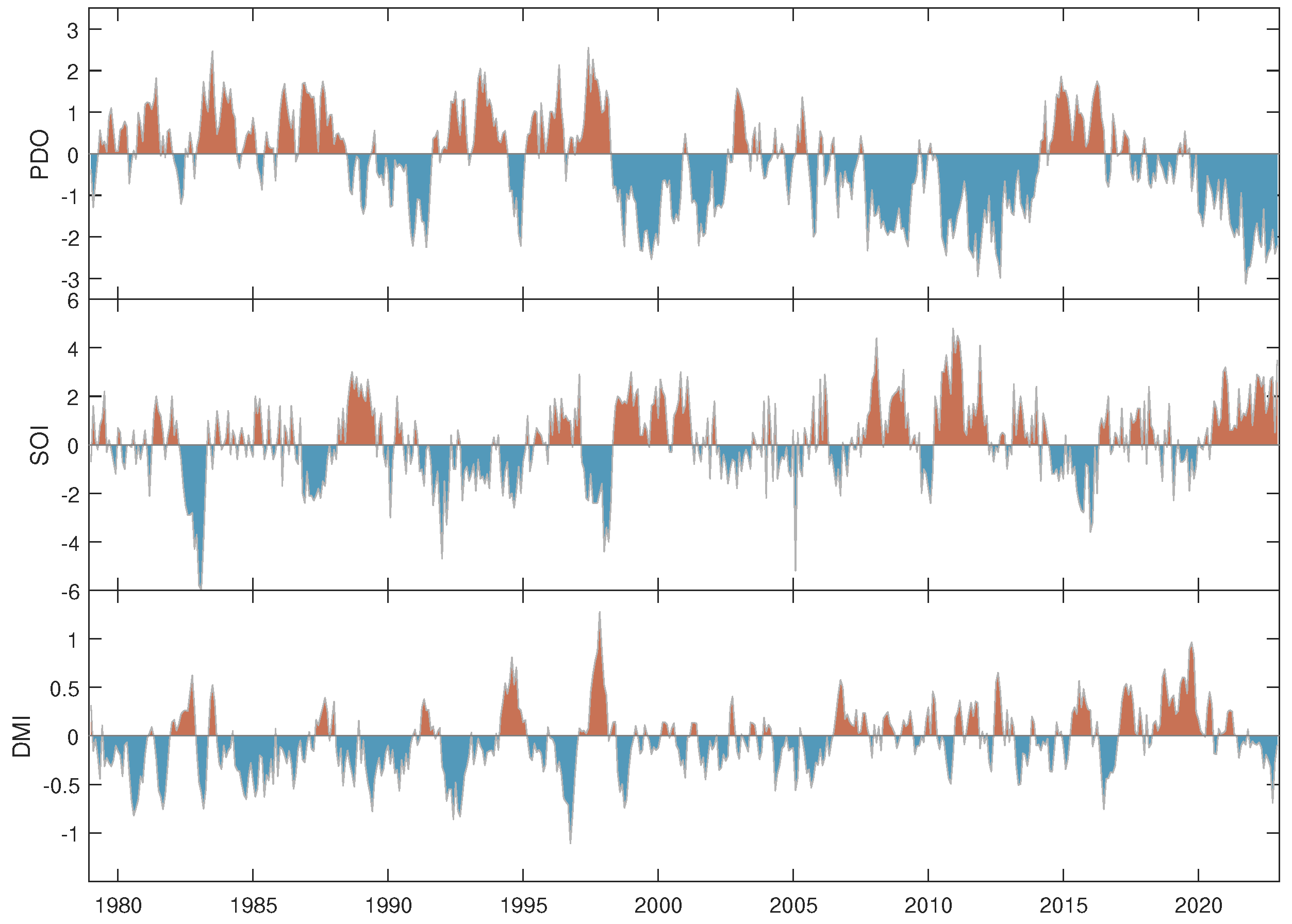
The PDO index is calculated by comparing sea surface temperature anomalies in different regions of the Pacific Ocean. A positive PDO index indicates warmer-than-average conditions in the central and eastern Pacific, while a negative index corresponds to cooler-than-average conditions. The monthly time series of the PDO index since 1854 can be obtained from the National Center for Environmental Information, NOAA (https://www.ncei.noaa.gov/access/monitoring/pdo/, (accessed on 15 March 2024)) (Figure 2).
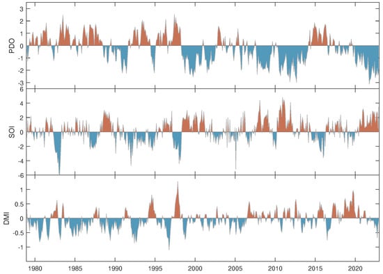
Figure 2.
The monthly time series of PDO, SOI, and DMI from 1979 to 2022.
The Southern Oscillation Index (SOI), a standardized difference between barometric pressures observed at stations in Darwin, Australia, and Tahiti, is used to quantify ENSO in this study. The negative phase of the SOI indicates below-normal air pressure at Tahiti and above-normal air pressure at Darwin. Prolonged periods of negative (positive) SOI values coincide with abnormally warm (cold) ocean waters across the eastern tropical Pacific, characteristic of El Niño (La Niña) episodes. The monthly SOI index could also be directly downloaded from the National Center for Environmental Information, NOAA (https://www.ncei.noaa.gov/access/monitoring/enso/soi, (accessed on 15 March 2024)) (Figure 2).
The Dipole Mode Index (DMI) is a metric used to quantify the strength and direction of the IOD in this study. This index measures the difference in sea surface temperatures between the eastern and western Central Indian Ocean, providing a numerical representation of the IOD’s intensity and phase. A positive DMI value indicates a positive IOD event, where the western Indian Ocean is warmer than usual and the eastern Indian Ocean is cooler. Conversely, a negative DMI value signifies a negative IOD event, with the temperature pattern reversed. The monthly SOI index could be accessed from https://psl.noaa.gov/gcos-wgsp/Timeseries/DMI/, (accessed on 15 March 2024) (Figure 2).
To understand the impact of climate variations on meteorological drought, we analyze the large-scale atmospheric circulation of mean geopotential height, air temperatures, and wind fields at 850 hPa from NCEP/NCAR Reanalysis datasets. These datasets are a comprehensive collection of atmospheric data jointly produced by the National Centers for Environmental Prediction (NCEP) and the National Center for Atmospheric Research (NCAR) in the United States. Created using the most advanced global data assimilation systems and extensive databases, these datasets process and homogenize observations from various sources, including ground stations, ships, radiosondes, wind-measuring balloons, aircraft, and satellites. They are reliable for climate analysis, especially since the beginning of the satellite era in 1979. The global dataset has a spatial resolution of 2.5° × 2.5° [46]. The integrated NCEP/NCAR Reanalysis datasets are available at http://www.esrl.noaa.gov/psd/data/, (accessed on 20 December 2023).
In this study, the sea surface temperature dataset used for climate analysis is the Extended Reconstructed Sea Surface Temperature (ERSST) v5, which provides a comprehensive record of global sea surface temperature variations from 1854 to 2024. This dataset is based on a combination of observations from various sources, including ship-based measurements, satellite observations, and buoy data. These observations are then combined and interpolated using sophisticated statistical techniques to create a seamless and continuous global SST record. This dataset is available at https://www.ncdc.noaa.gov/data-access, (accessed on 20 December 2023).
2.2. Methods
2.2.1. Stationarity Test
In this study, the stationarity of the precipitation and potential evaporation time series in March, April, and May from 1979 to 2022 (44 data points) were tested using the ADF test method, respectively [47,48]. The ADF tests were conducted through the ordinary least squares (OLS) estimation of regression models incorporating either an intercept or a linear trend. We considered the autoregressive model as follows:
where equals 0, and represents independent random variables with mean zero and variance . If , the time series is stationary. If , is nonstationary and represents a random walk process. The null hypothesis of the ADF test is , and more details can be found in [47,48].
2.2.2. Standardized Precipitation Evapotranspiration Index (SPEI)
SPEI provides a quantitative measure of drought severity and duration, considering both water supply (precipitation) and water demand (evapotranspiration) [12]. In this study, SPEI is calculated based on monthly climatic water balance, and the difference between precipitation (P) and potential evapotranspiration (). The next step is to fit a probability distribution to the cumulative water balance series. Then, the cumulative water balance values are transformed to the standard normal distribution to obtain the corresponding SPEI, where negative SPEI values indicate drought conditions, with the magnitude of the negativity representing the severity of the drought. In this study, the calculations of SPEI were performed by applying the R-package “SPEI” [49]. The SPEI can be further classified into different categories according to different thresholds; the specific classification criteria are listed in Table 1.

Table 1.
Drought classification based on the SPEI [12].
2.2.3. Coupled Climate Network Analysis
In this study, the interdependence between large-scale climate variability and droughts is first investigated by using a coupled climate network. SST in the North Pacific (32∼60° N, 130° E∼120° W) [50], tropical Pacific (−20° S∼20° N, 120° E∼80° W) [39], and tropical Indian Ocean (−10° S∼5° N, 40° E∼100° E) [51] are selected to represent PDO, ENSO, and IOD variations, respectively. The monthly SPEI time series over East Asia (15° N∼53° N, 100° E∼146° E) are chosen to represent droughts. This study area covers East China, the Korean Peninsula, Japan, and part of Russia.
The spatial fields of the two climate variables are described by two sets of univariate time series for SST and for SPEI, where each time series corresponds to the node in the coupled networks. The spatial resolutions of SST fields and SPEI fields are inherited from the SST and CRU TS 4.07 datasets. In this study, the linear relationships between SST and SPEI are evaluated by the Granger causality (GC) test. GC is defined as a causality test between two time series, SPEI and SST, in terms of the linear relationships between and the two lagged time series and for lags () [52,53]. The two linear models, which are, respectively, referred to as the complete model and the restricted model, are defined as follows:
and
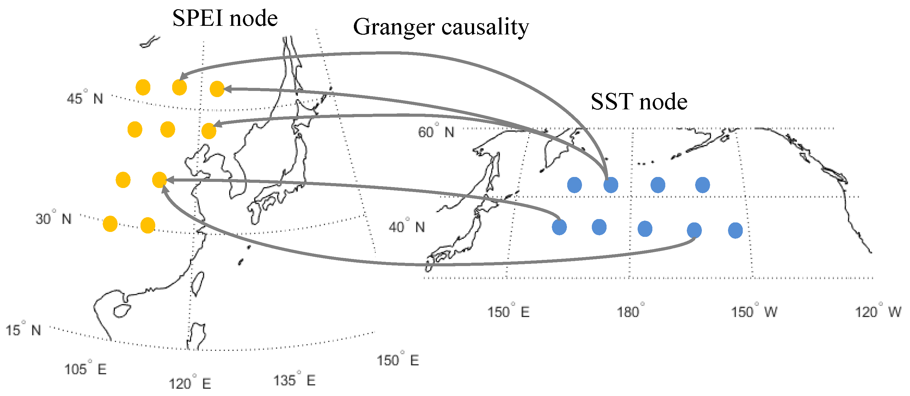
where , , and are constant model parameters, and and are white noise terms. The restricted model Equation (3) is regarded as the null model for the hypothesis that is not dependent on . Then, the hypothesis is tested by comparing the residuals of these two models: when the sum of the squared residuals for the complete model is significantly smaller than that for the restricted model , is thought to be caused by (denoted as ). Then, the matrix records the results of the GC test, and only 5% of links between SPEI and SST fields are kept for further network analysis, while the other 95% are discarded as non-significant links [54]. Then, the summation of each column of denotes the out-degree of the SST node, while the summation of each row denotes the in-degree of the SPEI node. The potential relationships between large-scale climate variations and SPEI can be partly revealed by the spatial patterns of out-degrees and in-degrees of the coupled climate networks. Figure 3 shows the schematic diagram of the coupled climate network between SST and SPEI.
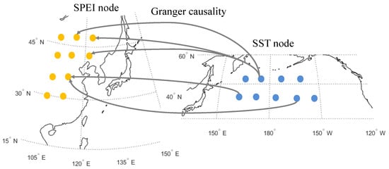
Figure 3.
The schematic diagram of the coupled climate network between SST and SPEI.
2.2.4. Composite Analysis
The climate variability indexes for the period from 1979 to 2022 are depicted in Figure 1. Utilizing these three time series, we have delineated the positive and negative phases of the PDO, SOI, and DMI. Specifically, for the PDO, thresholds of 1 and are set for the positive and negative phases. For the SOI, the thresholds are set at and , while for the DMI, they are and . To elucidate the influence of these large-scale climate variations on spring drought, we averaged the SPEI values for March, April, and May during the positive and negative phases of PDO, SOI, and DMI. By comparing these averaged SPEI values, we can identify the remote impacts of these climate variations on drought conditions. Additionally, we have averaged the atmospheric circulation anomalies around East Asia during these phases, relative to normal years, as referenced in [55]. For a composite analysis, this study considers three climate variables: geopotential height, air temperatures, and wind fields at the 850 hPa level.
3. Results
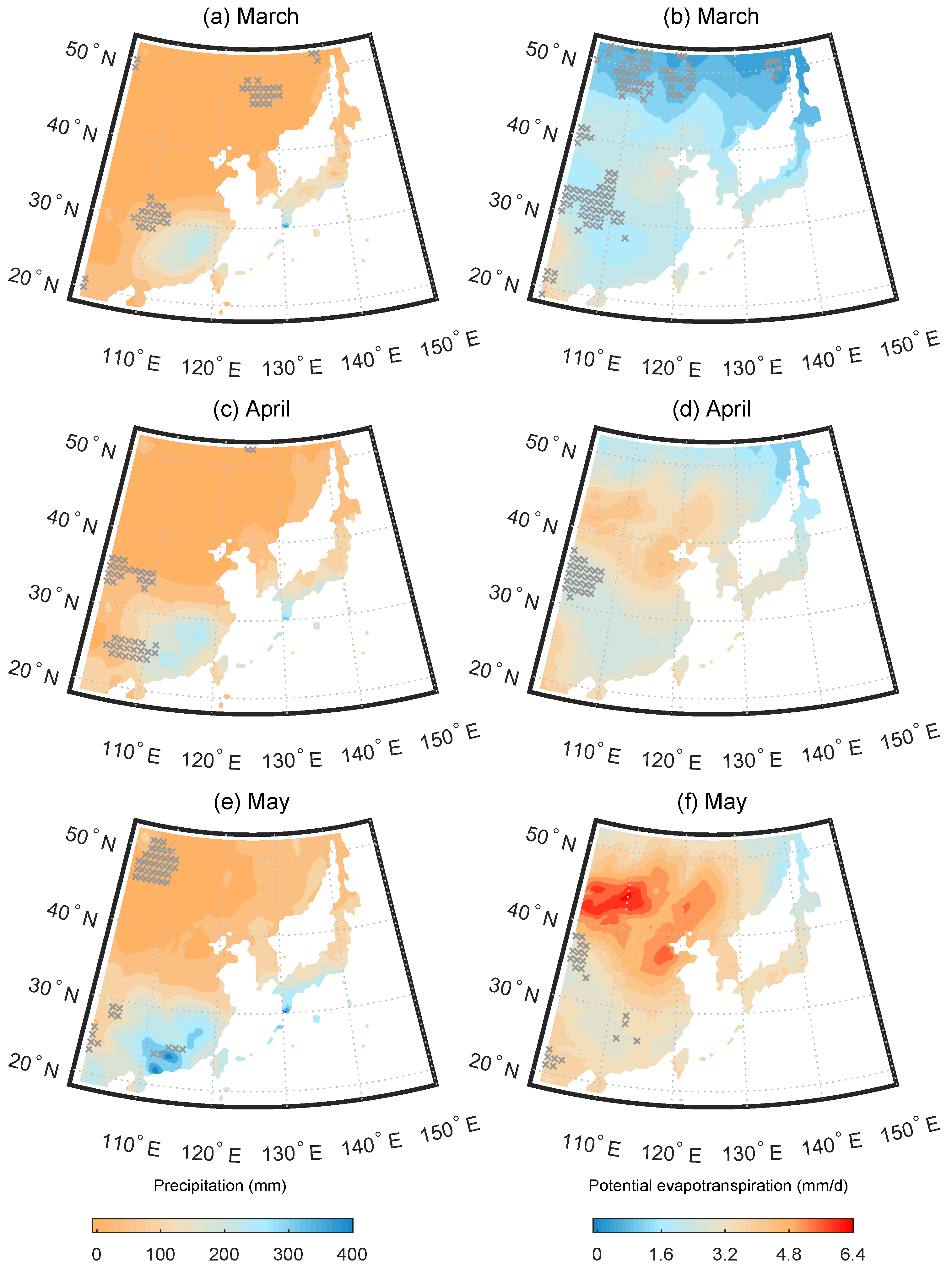
The averages of precipitation and potential evapotranspiration for March, April, and May are initially presented in Figure 4. Observing Figure 4, we notice that the precipitation distribution in the study area exhibits a gradient decrease from southeast to northwest during the three spring months. Along the southeast coast, precipitation rises from 200 mm to 400 mm between March and May. Conversely, in the northern part, the total precipitation does not exceed 100 mm in May, reflecting the semi-arid climate of this region. The latitudinal pattern is not as apparent for potential evapotranspiration. In March, the total potential evapotranspiration is relatively low and gradually increases in April and May. Notably, the areas with the highest potential evapotranspiration are located in Northern China, not necessarily the regions with higher latitudes where air temperatures are relatively lower. In particular, potential evapotranspiration can rise to 6.4 mm/day in May due to continuous sunny and hot weather, before the influence of the East Asian summer monsoon from the southeast arrives. However, this period coincides with the critical planting season for crops, which requires ample precipitation. Therefore, from a water resource management perspective, it is essential to ensure the efficient and rational utilization of water resources for agriculture in this semi-arid region. Additionally, Figure 4 reveals that most of the precipitation and potential evapotranspiration time series passed the augmented Dickey–Fuller (ADF) test at a significance level of , indicating their stationarity.

Figure 4.
The average precipitation (a,c,e) and potential evapotranspiration (b,d,f) in March, April, and May from 1979 to 2022. The stippling indicates the grids with nonstationary precipitation and potential evapotranspiration time series at the significance levels based on the ADF test.
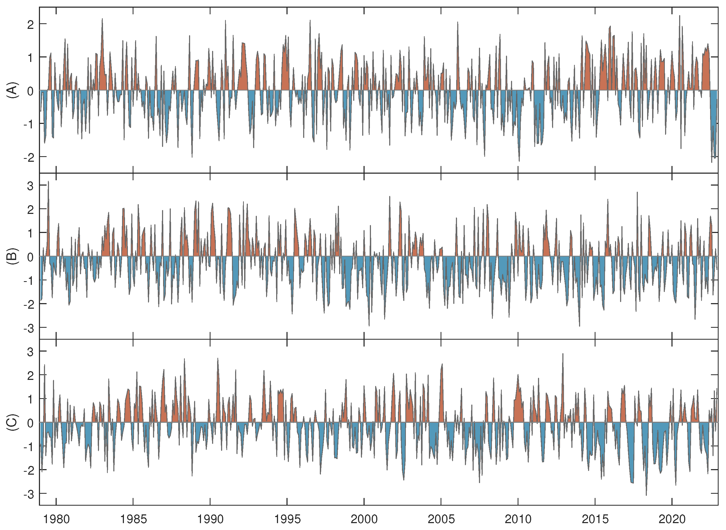
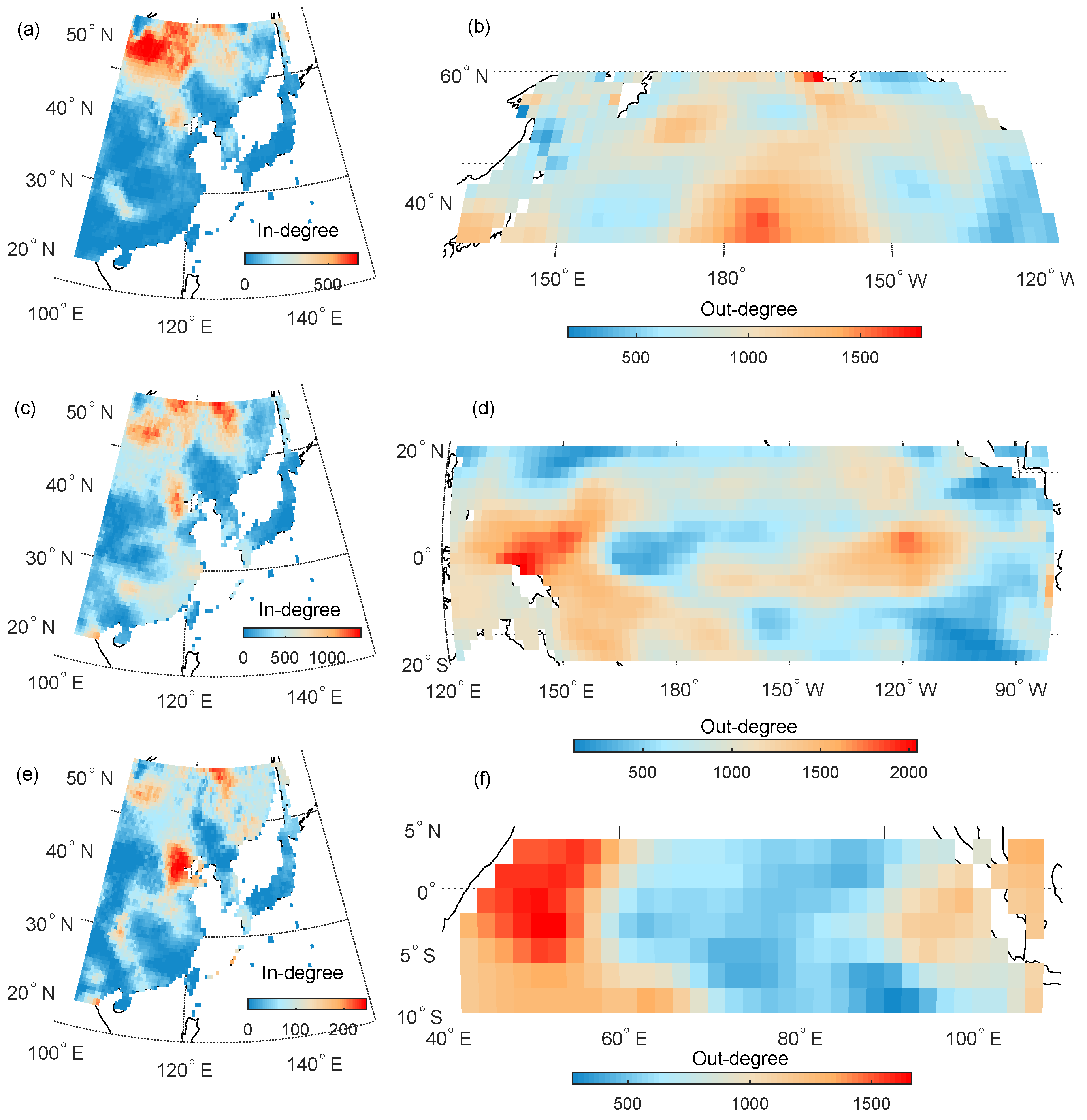
Based on the available precipitation and potential evapotranspiration data, we computed the SPEI from January 1979 to December 2022. In this study, the SPEI with a one-month time scale represents meteorological drought. Illustrative examples of the monthly SPEI time series for the three grid points, labeled (A), (B), and (C) in Figure 1, are presented in Figure 5. Subsequently, we calculate the Granger causality between the SPEI time series and sea surface temperature (SST) time series to construct coupled climate networks. Figure 6 depicts the in-degree of SPEI fields and out-degree of SST fields. Nodes with higher degree values connect more nodes on the other layer of the coupled network. The areas with higher in-degrees in the SPEI field correlate with areas with higher out-degrees in the SST field. Figure 5A,B indicate that droughts over Northern China and the Mongolian Plateau are correlated with the centers of the North Pacific and the Japan Sea. The spatial pattern of SST over the North Pacific is similar to the PDO spatial pattern [56], suggesting that the semi-arid region in East Asia is more sensitive to the remote impact of large-scale climate variability. The coupled climate network between SPEI and SST over the central Pacific also reveals the remote impact of the El Niño–Southern Oscillation (ENSO) on meteorological drought, as shown in Figure 6c,d. Specifically, the SST pattern in the coupled network aligns with the spatial SST pattern of ENSO reported in previous literature studies [54,57]. The area with the higher out-degree in the SST field is located at the eastern edge of the central Pacific. Additionally, the coupled climate network in Figure 6f reveals the spatial pattern of the Indian Ocean Dipole (IOD) [58]. By comparing Figure 6a,c,e, we find that high in-degrees are primarily distributed over the northern part of the study area. This finding suggests that droughts in semi-arid areas are more strongly correlated with large-scale climate variations.
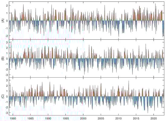
Figure 5.
Monthly SPEI time series from 1979 to 2022 for the three grid points labeled by (A), (B), and (C) in Figure 1, positive and negative values of SPEI are indicated by light brown and blue colors.
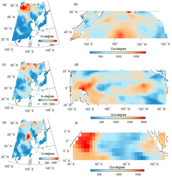
Figure 6.
In-degree fields of SPEI and out-degree fields of SST in the coupled climate networks. (a,b): East Asia vs. North Pacific; (c,d): East Asia vs. Central Pacific; (e,f): East Asia vs. Central Indian Ocean.
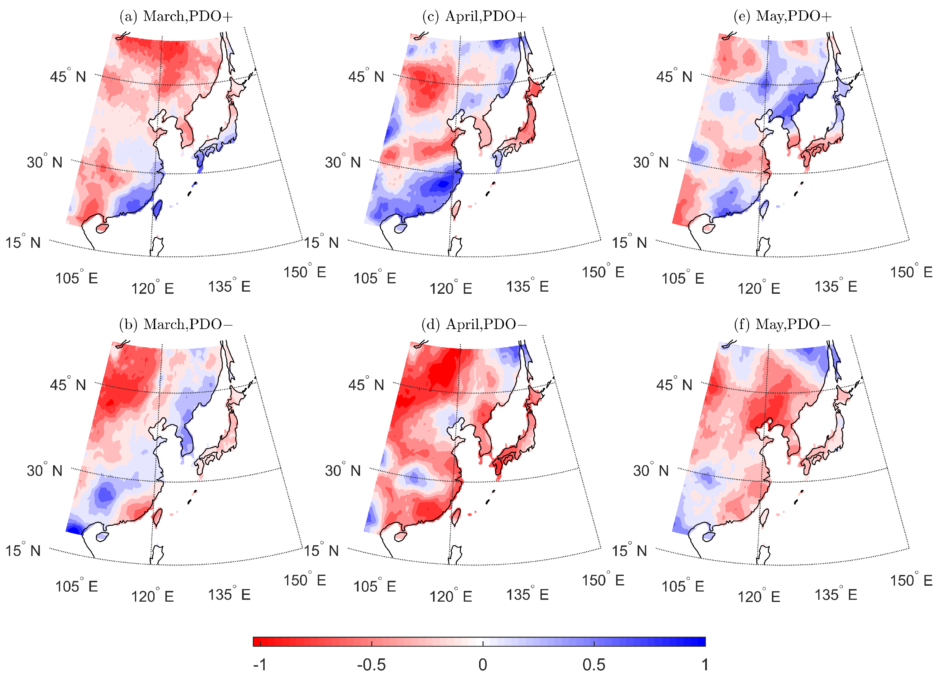
The average SPEI values for March, April, and May during the positive and negative phases of the PDO, SOI, and DMI are presented in Figure 7, Figure 8 and Figure 9, respectively. In the case of PDO, the spatial patterns of SPEI in March and April do not exhibit a complete reversal between the positive and negative phases. In March, droughts are prevalent, with relatively small wet areas. During the positive phase of PDO, a belt of wetter conditions emerges, spanning from the southeast coast of China to the south coast of Japan. In contrast, during the negative phase, this belt shifts northward, extending from South China to the Korean Peninsula and Northeast China. In April, drought conditions are more severe in the negative PDO phase compared to the positive phase. However, in May, the spatial pattern of SPEI in the positive and negative PDO phases begins to exhibit a more distinct opposition, with wetter areas in the positive phase tending to become drier in the negative phase, and vice versa. The proportions of each SPEI-based category of dryness/wetness during the positive and negative PDO phases in March, April, and May are summarized in Table 2. An opposing effect of positive and negative PDO on SPEI has been observed; Figure 7 and Table 2 do not indicate the presence of extreme wetness or dryness conditions.
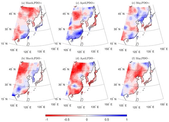
Figure 7.
Composite maps of SPEI for positive and negative phases of PDO in March, April, and May from 1979 to 2022.
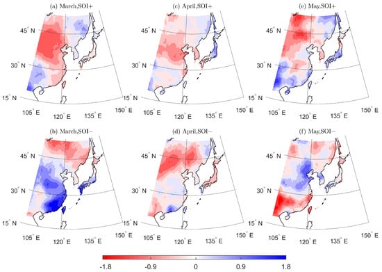
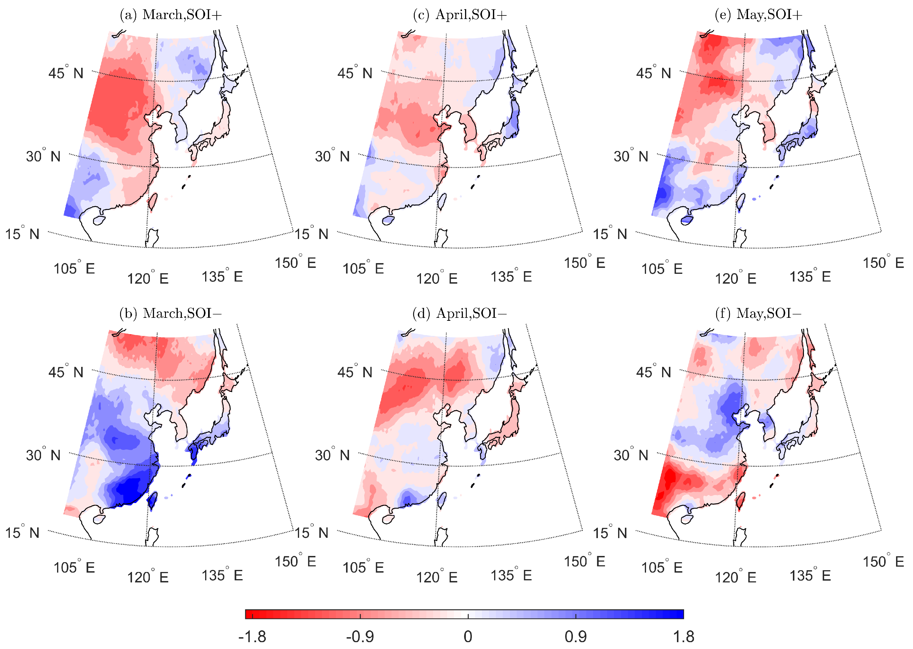
Figure 8.
The same as Figure 4 but for SOI.
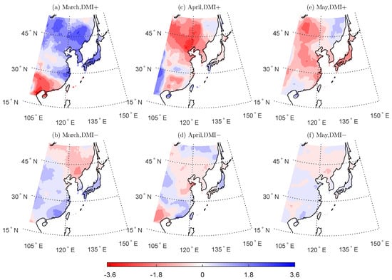
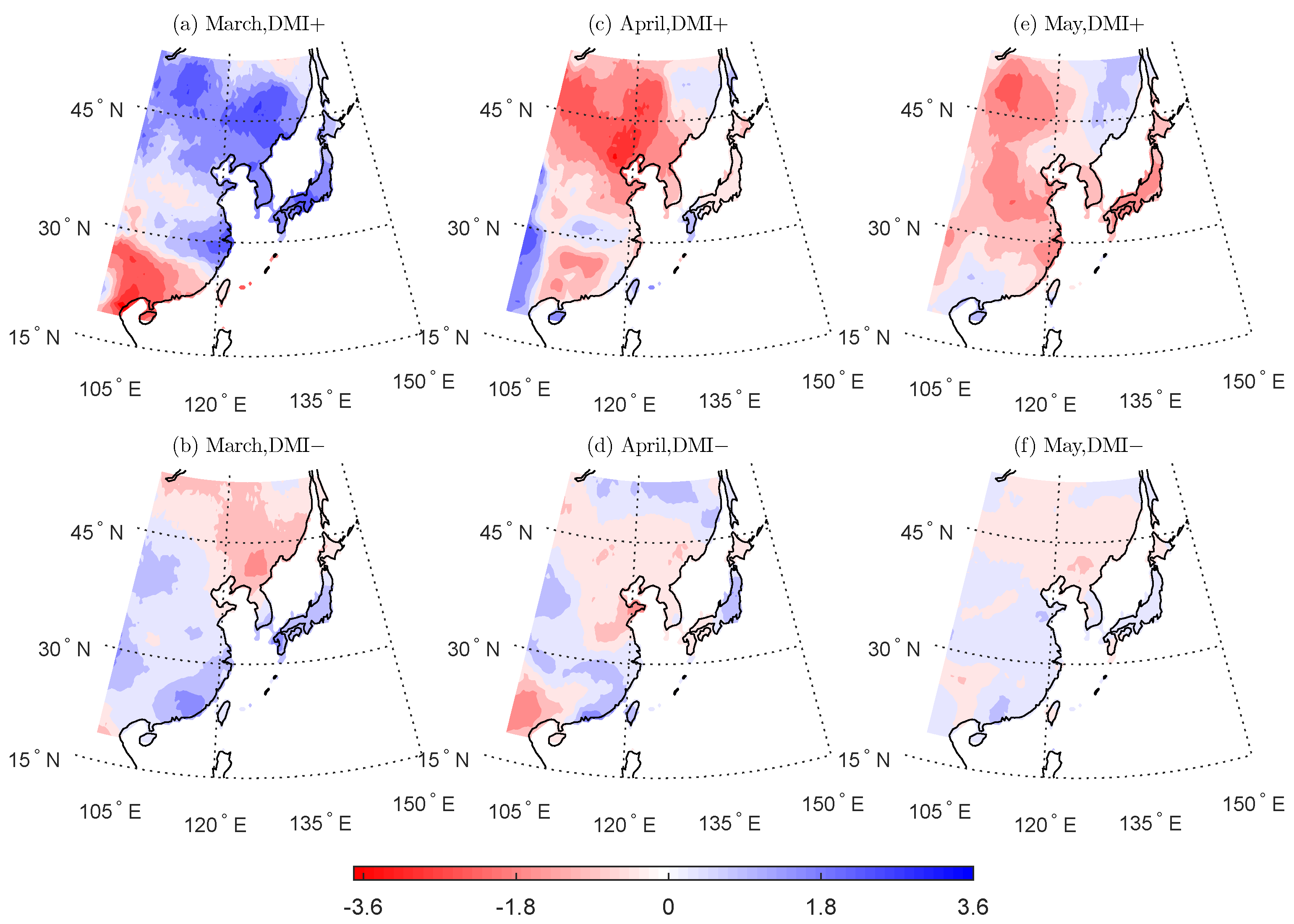
Figure 9.
The same as Figure 4 but for DMI.
Table 2.
The proportions of each category of dryness/wetness based on SPEI for positive and negative phases of PDO in March, April, and May (%).
In March, the remote impact of ENSO on SPEI over East Asia during the positive and negative phases is nearly opposite (Figure 8a,b). In the positive phase of SOI (La Niña), drought areas are primarily located in Northern China, while they shift northward to Northeast China and Russia in the negative phase of SOI (El Niño). In April, the drought area expands in both La Niña and El Niño phases, and the difference in their impact on SPEI over East Asia is not significant. However, in May, Southern China and Japan experience wetter conditions during La Niña but drier conditions during El Niño. In the El Niño phase, the wet area shifts to the central part of the study area, and drought conditions become less severe in the northern part. The remote impact of IOD on SPEI over East Asia in March, April, and May is inconsistent. During the positive phase of DMI, most of East Asia experiences wetter conditions in March but becomes drier in April and May (Figure 9). In the negative phase of DMI, the contrast between wet and dry areas in the spring season is less pronounced. Generally, the southern part of the study area tends to be wetter, while the northern part is drier. The proportions of each category of dryness/wetness based on SPEI during the positive and negative phases of SOI and DMI in March, April, and May are summarized in Table 3 and Table 4, respectively. It is noteworthy that extreme wetness or extreme dryness may occur in the positive phase of DMI in March and April.
Table 3.
The proportions of each category of dryness/wetness based on SPEI for positive and negative phases of SOI in March, April, and May (%).
Table 4.
The proportions of each category of dryness/wetness based on SPEI for positive and negative phases of DMI in March, April, and May (%).
4. Discussion
In this study, we focus on spring meteorological drought, a critical factor affecting agriculture in East Asia. Meteorological drought is primarily influenced by numerous climate factors, of which, the rainfall or snowfall amount, frequency, and distribution are pivotal in determining drought conditions [59]. Elevated temperatures accelerate evaporation rates, leading to faster drying of soil and water bodies, particularly in arid and semi-arid regions where evaporation rates are already high [60]. Wind patterns can also contribute to drought conditions, as strong winds can desiccate soil and plants, further aggravating drought’s impact [61]. Alterations in solar radiation and atmospheric composition, such as the increase in greenhouse gases, have a bearing on global climate patterns and temperatures. These changes, in turn, influence evaporation rates, precipitation patterns, and the occurrence of drought [61]. Additionally, large-scale atmospheric circulation patterns that govern the movement of moisture and precipitation play a significant role in drought conditions across vast regions [59,62,63]. Therefore, when analyzing a severe drought event, a comprehensive analysis of these climate factors is crucial to understanding the mechanisms leading to meteorological drought.
Oceanic processes, such as the spatial pattern of SST variability, have a profound influence on global climate patterns, including drought. These oceanic events can modulate atmospheric circulation and precipitation patterns, ultimately leading to drought or excessive rainfall [60,64]. Wu and Kinter [65] observed that SST can significantly impact both long- and short-term droughts in the Americas. Pan et al. [60] further demonstrated that the variation in compound drought and heat waves is linked to different SST modes. In this study, we explored the remote influence of three large-scale climate variations, PDO, ENSO, and IOD, on meteorological drought over East Asia. We constructed coupled climate networks analyzing two climate variables: SST and the SPEI. The spatial patterns of SST reflect the climate variations under investigation. PDO encapsulates changes in SST, wind patterns, and other oceanic and atmospheric variables that occur on a decadal timescale [66]. ENSO and SST patterns are closely intertwined, with ENSO events, such as El Niño and La Niña, significantly affecting SST patterns in the Pacific Ocean and beyond. For instance, during an El Niño event, SSTs in the eastern tropical Pacific increase significantly, while during a La Niña event, they cool. These temperature changes can then propagate to other regions of the globe, influencing SST patterns in those areas [67]. IOD is characterized by anomalous SST variations between the western and eastern regions of the Indian Ocean, with one side experiencing warmer waters and the other experiencing cooler waters [51]. Our analysis revealed that the out-degree of the SST field partly reflects the spatial pattern of SST representing the PDO, ENSO, and IOD variations. Furthermore, we found that drought in semi-arid regions is strongly correlated with these large-scale climate variations.
East Asia is greatly impacted by drought [43]. The are many studies focusing on the impact of these climate variations on temperature, precipitation, and drought in this study area. Wu et al. [44] analyzed the dynamic changes of the dryness/wetness characteristics in the Zhujiang river basin of South China and identified the roles of PDO and ENSO in determining drought in this area. Yang et al. [68] analyzed the spatiotemporal evolution patterns of droughts in China from 1961 to 2021 based on SPEI and found that drought has become weaker during this period. Wang et al. [17] analyzed the characteristics of the spatial and temporal distribution of drought in Northeast China during the same period. They also found that SPEI at the annual scale showed a decreasing trend. Hu et al. [22] identified the dominant patterns of dryness/wetness variability in the Huang-Huai-Hai River Basin of China and found that they were correlated with the multiscale climate oscillations. Atmospheric circulations are considered the leading factor in shaping the spatial pattern of dryness/wetness variability. Ge et al. [69] analyzed the characteristics and determining factors of spring–summer consecutive drought variations in Northwest China, and found that the change in atmospheric circulation was responsible for the change in drought. In this study, the impacts of PDO, ENSO, and IOD on spring drought were also analyzed from the perspective of atmospheric circulations. Meteorological droughts are also common in the Korean Peninsula and sometimes lead to hydrological droughts, agriculture droughts, or other secondary disasters [70,71].
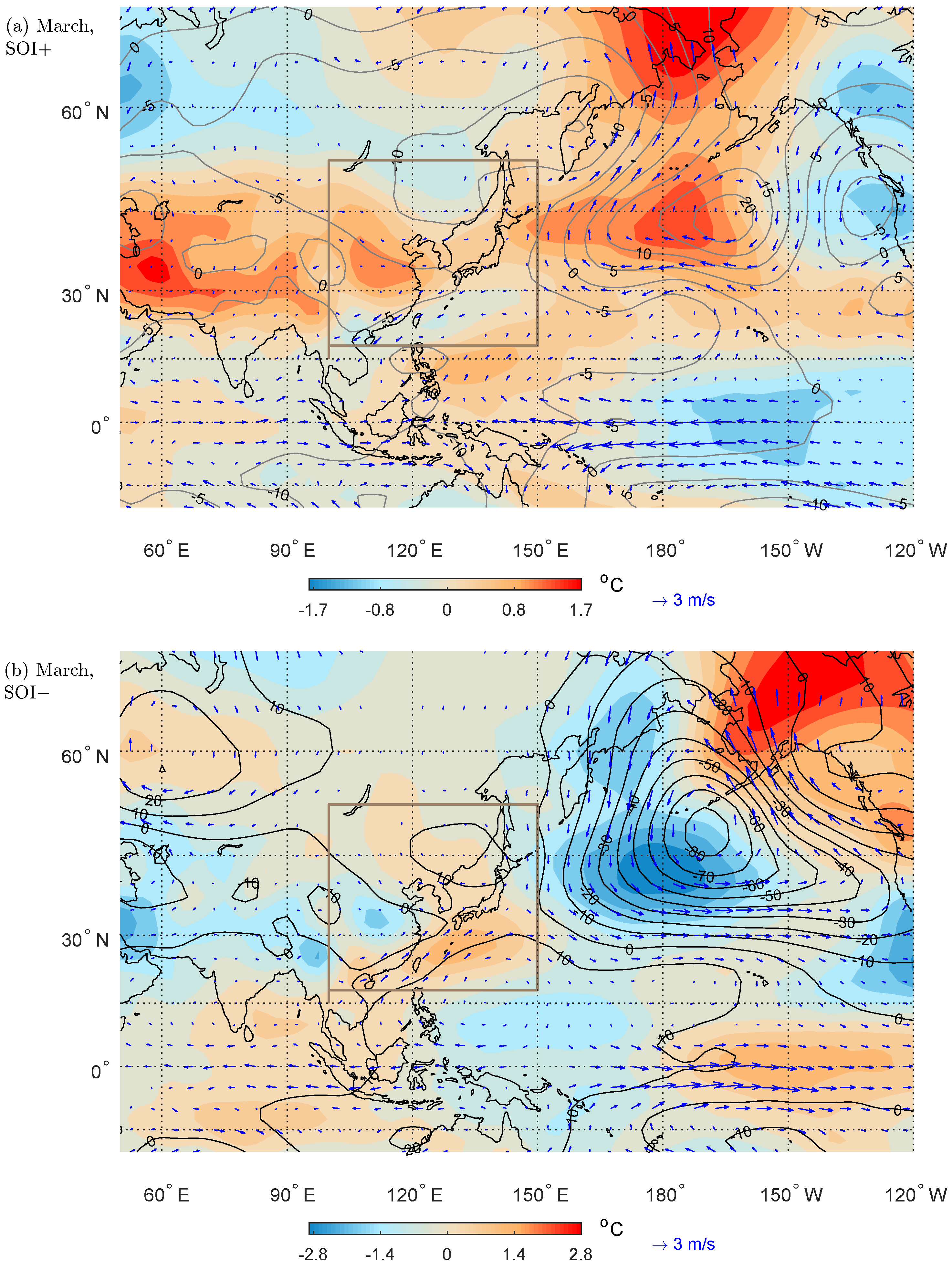
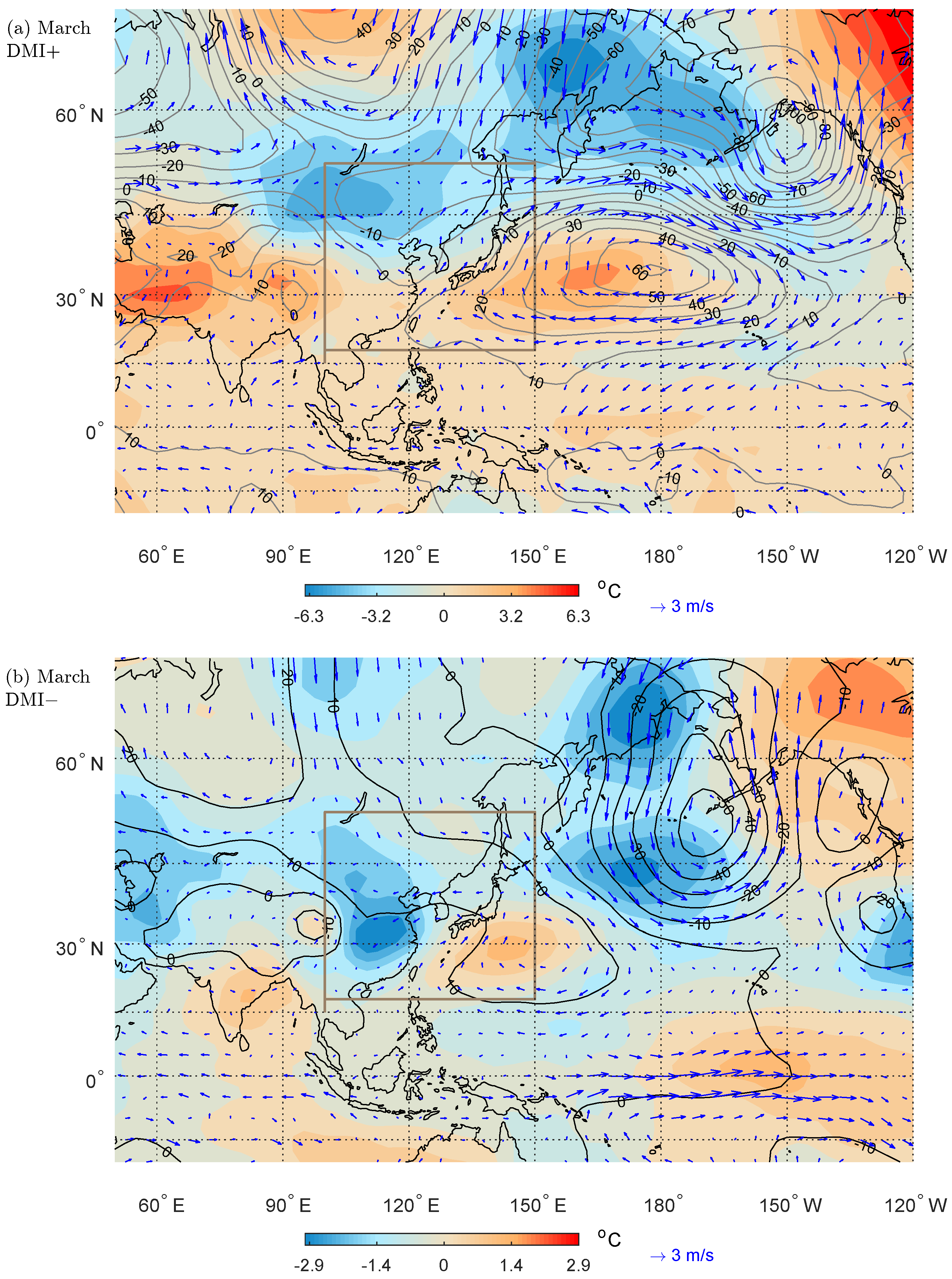
In this study, the remote impacts of PDO, ENSO, and IOD on spring meteorological drought over East Asia were revealed by composting the SPEI values for the positive and negative phases of these climate variations in March, April, and May, respectively. Previous studies have revealed that the PDO might exert a modulating effect on ENSO teleconnections in winter by shaping winter monsoon [72,73]. Also, the combined effect of IOD and ENSO is very complex [74]. Since we only focus on the spring meteorological drought from 1979 to 2022, the positive and negative of these three climate variations are not further distinguished into more classes. We speculated that the spatial patterns of spring meteorological drought could be partly explained by the atmospheric circulation patterns in different phases of climate variations. Figure 10, Figure 11 and Figure 12 present the atmospheric circulation anomalies for positive and negative phases of PDO, ENSO, and IOD in May and March, respectively. Figure 10a,b correspond to Figure 7e,f. Lower air temperatures, strong winds bringing moisture from the sea, and lower air pressures together contributed to the wet conditions, while higher air temperatures, strong winds without moisture, and higher air pressures are responsible for dry conditions. In addition, the atmospheric circulation anomalies presented in Figure 11a,b correspond to the composite maps of SPEI Figure 8a,b. The spatial patterns of air temperatures over the Central Pacific are consistent with the spatial pattern of SST in positive and negative phases of ENSO [75]. Moreover, higher/lower pressure centers associated with anti-cyclones and cyclones are located in the North Pacific. The large-scale circulation patterns partly explained the spatial pattern of drought in the positive phase of ENSO (La Niña). In the negative phase of ENSO (El Niño), Southern China and Japan are wet due to the warmer SST at the South/East China Sea and the southwest wind transporting vapor to South China and Japan. IOD is considered a counterpart to the climate-driving ENSO in the equatorial East Pacific. Yang et al. [76] and Wu et al. [77] both found the remote impact of IOD on summer precipitation over East Asia. Figure 12a,b correspond to Figure 9a,b. In the spring season, especially in March, the difference in atmospheric circulation patterns over the Indian Ocean is not obvious. Then the difference between SPEI patterns in positive and negative phases of DMI is probably explained by the air temperature anomalies. The only exception is Japan, which is wet in both the positive and negative phases of DMI due to the strong winds transporting vapor from warmer SST to land (Figure 12b).
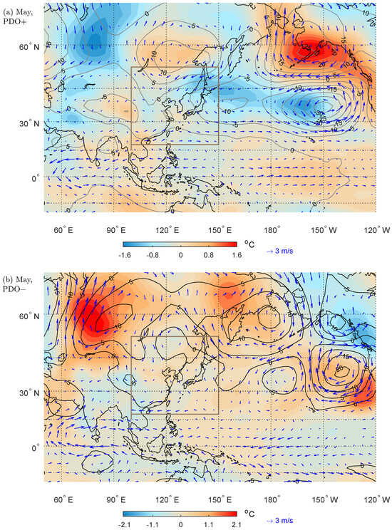
Figure 10.
Composite anomalies of geopotential height (gpm; contour with numbers), air temperature (°C; shaded), zonal and meridional wind anomalies (blue vectors) at 850-hPa level in positive (a) and negative phases (b) of PDO.
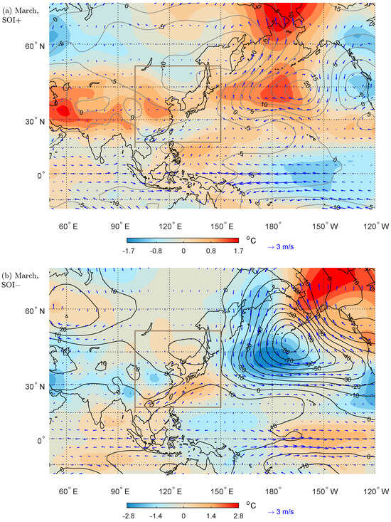
Figure 11.
The same as Figure 10 but for SOI.

Figure 12.
The same as Figure 10 but for DMI.
As the three major climate variations that significantly impact precipitation and temperature patterns over East Asia, the PDO, ENSO, and IOD are closely interrelated. PDO, a decadal climate pattern, can modulate the occurrence and strength of ENSO events. Research indicates that during specific phases of the PDO cycle, the frequency and magnitude of El Niño and La Niña events can undergo significant changes [73]. The correlation between ENSO and IOD is also complex but notable. There is a widely acknowledged positive correlation between the two phenomena. Specifically, during an El Niño event in the Pacific Ocean, there is a tendency for a positive IOD event to occur in the Indian Ocean during the same year’s summer and autumn [78,79]. In the future, the combined effects of these climate variations on drought should be examined on broader spatial and temporal scales.
In this study, the meteorological drought index used is the widely adopted SPEI, which traditionally assumes stationarity in probability distributions [12]. However, under the backdrop of a warming climate, this stationarity assumption has been increasingly violated [35]. Sun et al. [80] proposed a nonstationary SPEI by accounting for the non-stationarity of hydrometeorological processes. Similarly, in this study, the augmented Dickey–Fuller (ADF) test revealed that not all precipitation and potential evapotranspiration data are stationary. Previous studies have also detected changes in drought patterns [81]. In this research, the remote impact of the three climate variations was analyzed using coupled network analysis and composite analysis. As such, the non-stationarity of meteorological drought should also be taken into account in future studies.
5. Conclusions
East Asia is a region highly vulnerable to spring drought disasters, primarily due to the crucial role of agriculture in this area. In this study, we examined the remote effects of three large-scale climate variations, PDO, ENSO, and IOD, on spring meteorological drought over East Asia. Since these climate variations are reflected in SST patterns, we first constructed coupled climate networks between the SPEI and SST. Directed links from SST to SPEI were calculated using the Granger causality test, and only significant links were retained for network analysis. The out-degree of SST fields aligns with the spatial pattern of SST for these three climate variations, indicating that semi-arid areas are more sensitive to these large-scale climate variations.
In March and April, the effect of PDO on SPEI was not entirely opposing. However, in May, there were significant differences in the spatial patterns of SPEI between the positive and negative phases of PDO, though extreme wetness and dryness were not observed. In March, the remote impact of ENSO on SPEI over East Asia for positive and negative phases was almost the opposite. During the La Niña phase, drought areas were mainly concentrated in Northern China, while in the El Niño phase, they shifted northward to Northeast China and Russia. In April, the difference in the remote impact of ENSO on SPEI over East Asia was less apparent, and ENSO could lead to both severe wetness and severe dryness. While the remote impact of IOD on SPEI over East Asia in March, April, and May was inconsistent, IOD had the potential to cause extreme wetness and extreme dryness. Furthermore, we analyzed the impacts of PDO, ENSO, and IOD on spring drought from the perspective of atmospheric circulations. Generally, the wet or dry conditions over East Asia are determined by a combination of air temperatures, wind, and air pressure fields.
Author Contributions
Conceptualization, M.G.; methodology, M.G. and Y.W.; software, M.G.; validation, M.G. and Y.W.; formal analysis, M.G. and R.G.; investigation, M.G. and R.G.; resources, M.G.; data curation, M.G.; writing—original draft preparation, M.G.; writing—review and editing, M.G., R.G. and Y.W.; visualization, M.G.; supervision, M.G.; project administration, M.G.; funding acquisition, M.G. All authors have read and agreed to the published version of the manuscript.
Funding
This study was funded by the Key Program of Shandong Natural Science Foundation (no. ZR2020KF031).
Data Availability Statement
All the datasets used in this study can be freely accessed from the following websites: https://crudata.uea.ac.uk/cru/data/hrg/, accessed on 15 March 2024, https://www.ncei.noaa.gov93/access/monitoring/pdo/, accessed on 15 March 2024, https://www.ncei.noaa.gov/access/monitoring/enso/soi, accessed on 15 March 2024, https://psl.noaa.gov/gcos-wgsp/Timeseries/DMI/, accessed on 15 March 2024, http://www.esrl.noaa.gov/psd/data/, and https://www.ncdc.noaa.gov/data-access, accessed on 20 December 2023.
Conflicts of Interest
The authors declare no conflicts of interest.
Abbreviations
| SPEI | standardized precipitation evapotranspiration index |
| PDO | Pacific Decadal Oscillation |
| ENSO | El Niño–Southern Oscillation |
| SOI | Southern Oscillation Index |
| IOD | Indian Ocean Dipole |
| DMI | Dipole Mode Index |
| SST | sea surface temperature |
| GC | Granger causality |
References
- Trenberth, K.E.; Dai, A.; Van Der Schrier, G.; Jones, P.D.; Barichivich, J.; Briffa, K.R.; Sheffield, J. Global Warming and Changes in Drought. Nat. Clim. Chang. 2014, 4, 17–22. [Google Scholar] [CrossRef]
- Otop, I.; Adynkiewicz-Piragas, M.; Zdralewicz, I.; Lejcu s, I.; Miszuk, B. The Drought of 2018–2019 in the Lusatian Neisse River Catchment in Relation to the Multiannual Conditions. Water 2023, 15, 1647. [Google Scholar] [CrossRef]
- Dai, A. Increasing Drought under Global Warming in Observations and Models. Nat. Clim. Chang. 2013, 3, 52–58. [Google Scholar] [CrossRef]
- El Qorchi, F.; Yacoubi Khebiza, M.; Omondi, O.A.; Karmaoui, A.; Pham, Q.B.; Acharki, S. Analyzing Temporal Patterns of Temperature, Precipitation, and Drought Incidents: A Comprehensive Study of Environmental Trends in the Upper Draa Basin, Morocco. Water 2023, 15, 3906. [Google Scholar] [CrossRef]
- Wilhite, D.A.; Glantz, M.H. Understanding: The Drought Phenomenon: The Role ff Definitions. Water Int. 1985, 10, 111–120. [Google Scholar] [CrossRef]
- Haile, G.G.; Tang, Q.; Li, W.; Liu, X.; Zhang, X. Drought: Progress in Broadening its Understanding. Wiley Interdiscip. Rev. Water 2020, 7, e1407. [Google Scholar] [CrossRef]
- Wang, Y.; Zhang, J.; Guo, E.; Dong, Z.; Quan, L. Estimation of Variability Characteristics of Regional Drought during 1964–2013 in Horqin Sandy Land China. Water 2016, 8, 543. [Google Scholar] [CrossRef]
- Herrera-Estrada, J.E.; Satoh, Y.; Sheffield, J. Spatiotemporal Dynamics of Global Drought. Geophys. Res. Lett. 2017, 44, 2254–2263. [Google Scholar] [CrossRef]
- Gibbs, W.J.; Maher, J.V. Rainfall Deciles as Drought Indicators. Bureau of Meteorology; Commonwealth of Australia: Melbourne, Australia, 1967.
- Palmer, W.C. Meteorological Drought; US Department of Commerce, Weather Bureau: Silver Spring, MD, USA, 1965.
- McKee, T.B.; Doesken, N.J.; Kleist, J. The Relationship of Drought Frequency and Duration to Time Scales. In Proceedings of the 8th Conference on Applied Climatology, Anaheim, CA, USA, 17–22 January 1993; American Meteorological Society: Anaheim, CA, USA, 1993. [Google Scholar]
- Vicente-Serrano, S.M.; Beguería, S.; López-Moreno, J.I. A Multiscalar Drought Index Sensitive to Global Warming: The Standardized Precipitation Evapotranspiration Index. J. Clim. 2010, 23, 1696–1718. [Google Scholar] [CrossRef]
- Yu, H.; Zhang, Q.; Xu, C.-Y.; Du, J.; Sun, P.; Hu, P. Modified Palmer Drought Severity Index: Model Improvement and Application. Environ. Int. 2019, 130, 104951. [Google Scholar] [CrossRef]
- Santos, J.F.; Tadic, L.; Portela, M.M.; Espinosa, L.A.; Brleković, T. Drought Characterization in Croatia Using E-OBS Gridded Data. Water 2023, 15, 3806. [Google Scholar] [CrossRef]
- Liu, X.; Zhu, X.; Pan, Y.; Bai, J.; Li, S. Performance of Different Drought Indices for Agriculture Drought in the North China Plain. J. Arid. Land. 2018, 10, 507–516. [Google Scholar] [CrossRef]
- Zhang, W.; Wang, Z.; Lai, H.; Men, R.; Wang, F.; Feng, K.; Qi, Q.; Zhang, Z.; Quan, Q.; Huang, S. Dynamic Characteristics of Meteorological Drought and Its Impact on Vegetation in an Arid and Semi-Arid Region. Water 2023, 15, 3882. [Google Scholar] [CrossRef]
- Wang, R.; Zhang, X.; Guo, E.; Cong, L.; Wang, Y. Characteristics of the Spatial and Temporal Distribution of Drought in Northeast China, 1961–2020. Water 2024, 16, 234. [Google Scholar] [CrossRef]
- Das, P.K.; Dutta, D.; Sharma, J.R.; Dadhwal, V.K. Trends and Behaviour of Meteorological Drought (1901–2008) over Indian Region Using Standardized Precipitation—Evapotranspiration Index. Int. J. Climatol. 2016, 36, 909–916. [Google Scholar] [CrossRef]
- Bao, G.; Liu, Y.; Liu, N.; Linderholm, H. Drought Variability in Eastern Mongolian Plateau and its Linkages To The Large-Scale Climate Forcing. Clim. Dyn. 2015, 44, 717–733. [Google Scholar] [CrossRef]
- Wu, J.; Chen, X. Spatiotemporal Trends of Dryness/Wetness Duration and Severity: The Respective Contribution of Precipitation and Temperature. Atmos. Res. 2019, 216, 176–185. [Google Scholar] [CrossRef]
- Beguería, S.; Vicente-Serrano, S.; Reig, F.; Latorre, B. Standardized Precipitation Evapotranspiration Index (Spei) Revisited: Parameter Fitting, Evapotranspiration Models, Tools, Datasets and Drought Monitoring. Int. J. Climatol. 2014, 34, 3001–3023. [Google Scholar] [CrossRef]
- Hu, W.; She, D.; Xia, J.; He, B.; Hu, C. Dominant Patterns of Dryness/Wetness Variability In The Huang-Huai-Hai River Basin and its Relationship with Multiscale Climate Oscillations. Atmos. Res. 2021, 247, 105148. [Google Scholar] [CrossRef]
- Manzano, A.; Clemente, M.A.; Morata, A.; Luna, M.Y.; Beguería, S.; Vicente-Serrano, S.M.; Martín, M.L. Analysis of the Atmospheric Circulation Pattern Effects over SPEI Drought Index in Spain. Atmos. Res. 2019, 230, 104630. [Google Scholar] [CrossRef]
- Mishra, A.K.; Singh, V.P. A Review of Drought Concepts. J. Hydrol. 2010, 391, 202–216. [Google Scholar] [CrossRef]
- Ma, B.; Zhang, B.; Jia, L.; Huang, H. Conditional Distribution Selection For Spei-Daily and Its Revealed Meteorological Drought Characteristics in China from 1961 to 2017. Atmos. Res. 2020, 246, 105108. [Google Scholar] [CrossRef]
- Available online: https://www.stats.gov.cn/ (accessed on 10 May 2024).
- Available online: https://www.statista.com/statistics/645885/japan-rice-production-volume/ (accessed on 10 May 2024).
- Zhao, Q.; Yang, S.; Tian, H.; Deng, K. Leading Pattern of Spring Drought Variability over East Asia and Associated Drivers. J. Trop. Meteorol. 2024, 30, 1–10. [Google Scholar]
- Son, J.H.; Seo, K.H. East Asian Summer Monsoon Precipitation Response to Variations in Upstream Westerly Wind. Clim. Dynam. 2022, 59, 77–84. [Google Scholar] [CrossRef]
- Deng, Y.; Gao, L.L.; Gou, X.H. Spatiotemporal Drought Variation in Midlatitude East Asia over the Past Half Millennium. J. Geophys. Res. 2023, 128, e2022JD037793. [Google Scholar] [CrossRef]
- Guo, E.; Liu, X.; Zhang, J.; Wang, Y.; Wang, Y.; Wang, C.; Wang, R.; Li, D. Assessing Spatiotemporal Variation of Drought and Its Impact on Maize Yield in Northeast China. J. Hydrol. 2017, 553, 231–247. [Google Scholar] [CrossRef]
- Shi, W.; Wang, M.; Liu, Y. Crop Yield and Production Responses to Climate Disasters in China. Sci. Total Environ. 2021, 750, 141147. [Google Scholar] [CrossRef] [PubMed]
- Kiem, A.S.; Franks, S.W.; Kuczera, G. Multi-Decadal Variability of Flood Risk. Geophys. Res. Lett. 2003, 30, GL015992. [Google Scholar] [CrossRef]
- Villafuerte, M.Q., II; Matsumoto, J.; Akasaka, I.; Takahashi, H.G.; Kubota, H.; Cinco, T.A. Long-Term Trends And Variability of Rainfall Extremes in the Philippines. Atmos. Res. 2014, 137, 1–13. [Google Scholar] [CrossRef]
- Gao, M.; Mo, D.; Wu, X. Nonstationary Modeling of Extreme Precipitation in China. Atmos. Res. 2016, 182, 1–9. [Google Scholar] [CrossRef]
- Gao, M.; Zheng, H. Nonstationary extreme Value Analysis of Temperature Extremes in China. Stoch. Environ. Res. Risk Assess. 2018, 32, 1299–1315. [Google Scholar] [CrossRef]
- Wei, W.; Yang, Z.; Li, Z. Influence of Pacific Decadal Oscillation on Global Precipitation Extremes. Environ. Res. Lett. 2021, 16, 044031. [Google Scholar] [CrossRef]
- Trenberth, K.E.; Stepaniak, D.P. Indices of El Niño Southern Oscillation and Tropical Atlantic Sea Surface Temperature Anomalies. J. Clim. 2001, 14, 1686–1701. [Google Scholar]
- Yeh, S.W.; Kug, J.S.; Dewitte, B.; Kim, S.Y.; Jin, F.F.; An, S.I. El Niño in Changing Climate. Nature 2009, 461, 511–514. [Google Scholar] [CrossRef] [PubMed]
- Cai, W.; Borlace, S.; Lengaigne, M.; van Rensch, P.; Collins, M.; Vecchi, G.A.; Jin, F.F. Increasing Frequency of Extreme El Niño Events Due To Greenhouse Warming. Nature 2014, 510, 633–637. [Google Scholar] [CrossRef] [PubMed]
- Jiang, Y.; Zhou, L.; Roundy, P.E.; Hua, W.; Raghavendra, A. Increasing Influence of Indian Ocean Dipole on Precipitation over Central Equatorial Africa. Geophys. Res. Lett. 2021, 48, e2020GL092370. [Google Scholar] [CrossRef]
- Zhang, Y.; Zhou, W.; Wang, X.; Chen, S.; Chen, J.; Li, S. Indian Ocean Dipole and ENSO’s Mechanistic Importance in Modulating The Ensuing-Summer Precipitation over Eastern China. NPJ Clim. Atmos. Sci. 2022, 5, 48. [Google Scholar] [CrossRef]
- Zhang, L.; Zhou, T. Drought over East Asia: A Review. J. Clim. 2015, 28, 3375–3399. [Google Scholar] [CrossRef]
- Wu, J.; Tan, X.; Chen, X.; Lin, K. Dynamic Changes of The Dryness/Wetness Characteristics in The Largest River Basin of South China and Their Possible Climate Driving Factors. Atmos. Res. 2020, 232, 104685. [Google Scholar] [CrossRef]
- Yang, P.; Wang, W.; Xia, J.; Zhang, Y.; Zhan, C.; Zhang, S.; Chen, N.; Luo, H.; Li, J. Linear and Nonlinear Causal Relationships between the Dry/Wet Conditions and Teleconnection Indices in the Yangtze River Basin. Atmos. Res. 2022, 275, 106249. [Google Scholar] [CrossRef]
- Leetmaa, A.; Reynolds, R.; Jenne, R.; Josepht, D. The NCEP/NCAR 40-year Reanalysis Project. Bull. Am. Meteorol. Soc. 1996, 77, 437–471. [Google Scholar]
- Dickey, D.A.; Fuller, W.A. Distribution of the Estimators for Autoregressive Time Series with a Unit Root. J. Am. Stat. Assoc. 1979, 74, 423–431. [Google Scholar]
- Said, S.E.; Dickey, D. Testing for Unit Roots in Autoregressive Moving-Average Models with Unknown Order. Biometrika 1984, 71, 599–607. [Google Scholar] [CrossRef]
- SPEI. Available online: https://github.com/sbegueria/SPEI (accessed on 2 April 2024).
- Lu, Z.; Yuan, N.; Yang, Q.; Ma, Z.; Kurths, J. Early warning of the Pacific Decadal Oscillation Phase Transition using Complex Network Analysis. Geophys. Res. Lett. 2021, 48, e2020GL091674. [Google Scholar] [CrossRef]
- Saji, N.H.; Goswami, B.N.; Vinayachandran, P.N.; Yamagata, T. A Dipole Mode in The Tropical Indian Ocean. Nature 1999, 401, 360–363. [Google Scholar] [CrossRef] [PubMed]
- Silva, F.N.; Vega-Oliveros, D.A.; Yan, X.; Flammini, A.; Menczer, F.; Radicchi, F.; Kravitz, B.; Fortunato, S. Detecting Climate Teleconnections with Granger causality. Geophys. Res. Lett. 2021, 48, e2021GL094707. [Google Scholar] [CrossRef]
- Hamilton, J.D. Time Series Analysis. Princeton; Princeton University Press: Princeton, NJ, USA, 1994. [Google Scholar]
- Gao, M.; Zhao, Y.; Wang, Z.; Wang, Y. A Modified Extreme Event-Based Synchronicity Measure for Climate Time Series. Chaos 2023, 33, 023105. [Google Scholar] [CrossRef]
- Yang, Y.; Gao, M.; Xie, N.; Gao, Z. Relating anomalous Large-Scale Atmospheric Circulation Patterns to Temperature and Precipitation Anomalies in the East Asian Monsoon Region. Atmos. Res. 2020, 232, 104679. [Google Scholar] [CrossRef]
- Dong, X. Influences of the Pacific Decadal Oscillation on the East Asian Summer Monsoon in non-ENSO Years. Atmos. Sci. Lett. 2016, 17, 115–120. [Google Scholar] [CrossRef]
- Timmermann, A.; An, S.I.; Kug, J.S.; Jin, F.F.; Cai, W.; Capotondi, A.; Cobb, K.M.; Lengaigne, M.; McPhaden, M.J.; Stuecker, M.F.; et al. El Niño–southern Oscillation Complexity. Nature 2018, 559, 535–545. [Google Scholar] [CrossRef]
- Basharin, D.; Stankūnavičius, G. European Precipitation Response to Indian Ocean Dipole Events. Atmos. Res. 2022, 273, 106142. [Google Scholar] [CrossRef]
- Irfan, U.; Xieyao, M.; Jun, Y.; Abubaker, O.; Asmerom, H.B.; Farhan, S.; Vedaste, I.; Sidra, S.; Muhammad, A.; Mengyang, L. Spatiotemporal Characteristics of Meteorological Drought Variability and trends (1981–2020) over South Asia and the associated large-scale circulation patterns. Clim. Dynam. 2023, 60, 2261–2284. [Google Scholar]
- Pan, X.; Wang, W.; Shao, Q.; Wei, J.; Li, H.; Zhang, F.; Cao, M.; Yang, L. Compound Drought and Heat Waves Variation and Association with Sst Modes across China. Sci. Total Environ. 2024, 907, 167934. [Google Scholar] [CrossRef] [PubMed]
- Richardson, D.; Pitman, A.J.; Ridder, N.N. Climate Influence on Compound Solar and Wind Droughts in Australia. NPJ Clim. Atmos. Sci. 2023, 6, 184. [Google Scholar] [CrossRef]
- Zhang, Y.; You, Q.; Lin, H.; Chen, C. Analysis of Dry/Wet Conditions in the Gan River Basin, China, and Their Association with Large-Scale Atmospheric Circulation. Global Planet Chang. 2015, 133, 309–317. [Google Scholar] [CrossRef]
- Hamal, K.; Sharma, S.; Pokharel, B.; Shrestha, D.; Talchabhadel, R.; Shrestha, A.; Khadka, N. Changing Pattern of Drought in Nepal and Associated Atmospheric Circulation. Atmos. Res. 2021, 262, 105798. [Google Scholar] [CrossRef]
- Ionita, M.; Nagavciuc, V.; Scholz, P.; Dima, M. Long-term Drought Intensification over Europe Driven by the Weakening Trend of the Atlantic Meridional Overturning Circulation. J. Hydrol. Reg. Stud. 2022, 42, 101176. [Google Scholar] [CrossRef]
- Wu, R.; Kinter, J.L., III. Analysis of the Relationship of U.S. Droughts with SST and Soil Moisture: Distinguishing the Time Scale of Droughts. J. Clim. 2009, 22, 4520–4538. [Google Scholar] [CrossRef]
- Mantua, N.J.; Hare, S.R.; Zhang, Y.; Wallace, J.M.; Francis, R.C. A Pacific Interdecadal Climate Oscillation with Impacts on Salmon Production. Bull. Am. Meteorol. Soc. 1997, 78, 1069–1079. [Google Scholar] [CrossRef]
- Dai, A.; Wigley, T.M.L. Global patterns of ENSO-induced precipitation. Geophys. Res. Lett. 2000, 27, 1283–1286. [Google Scholar] [CrossRef]
- Yang, Y.; Dai, E.; Yin, J.; Jia, L.; Zhang, P.; Sun, J. Spatial and Temporal Evolution Patterns of Droughts in China over the Past 61 Years Based on the Standardized Precipitation Evapotranspiration Index. Water 2024, 16, 1012. [Google Scholar] [CrossRef]
- Ge, J.; Feng, D.; Liu, H.; Li, W.; Zhu, Y. Characteristics and Determining Factors of Spring-Summer Consecutive Drought Variations in Northwest China. Atmos. Res. 2024, 304, 107361. [Google Scholar] [CrossRef]
- Nam, W.H.; Hayes, M.J.; Svoboda, M.D.; Tadesse, T.; Wilhite, D.A. Drought Hazard Assessment In The Context of Climate Change for South Korea. Agric. Water Manag. 2015, 160, 106–117. [Google Scholar] [CrossRef]
- Seo, J.; Won, J.; Lee, H.; Kim, S. Probabilistic Monitoring of Meteorological Drought Impacts on Water Quality of Major Rivers in South Korea using Copula Models. Water Res. 2024, 251, 121175. [Google Scholar] [CrossRef]
- Wang, L.; Chen, W.; Huang, R. Interdecadal modulation of PDO on the Impact Of ENSO On The East Asian Winter Monsoon. Geophys. Res. Lett. 2008, 35, L20702. [Google Scholar] [CrossRef]
- Kim, J.W.; Yeh, S.W.; Chang, E.C. Combined effect of El Niño-Southern Oscillation and Pacific Decadal Oscillation on the East Asian Winter Monsoon. Clim. Dynam. 2013, 42, 957–971. [Google Scholar] [CrossRef]
- Yin, H.; Wu, Z.; Fowler, H.J.; Blenkinsop, S.; He, H.; Li, Y. The Combined Impacts of ENSO and IOD on Global Seasonal Droughts. Atmosphere 2022, 13, 1673. [Google Scholar] [CrossRef]
- Chen, Y.; Zhao, Y.; Feng, J.; Wang, F. ENSO Cycle and Climate Anomaly in China. Chin. J. Oceanol. Limn. 2012, 30, 985–1000. [Google Scholar] [CrossRef]
- Yang, J.; Liu, Q.; Liu, Z. Linking observations of the Asian monsoon to the Indian Ocean SST: Possible roles of Indian Ocean Basin mode and dipole mode. J. Clim. 2010, 23, 5889–5902. [Google Scholar] [CrossRef]
- Wu, R.; Yang, S.; Wen, Z.; Huang, G.; Hu, K. Interdecadal change in the relationship of southern China summer rainfall with tropical Indo-Pacific SST. Theor. Appl. Climatol. 2012, 108, 119–133. [Google Scholar] [CrossRef]
- Stuecker, M.F.; Timmermann, A.; Jin, F.F.; Chikamoto, Y.; Zhang, W.; Wittenberg, A.T.; Widiasih, E.; Zhao, S. Revisiting ENSO/Indian Ocean Dipole phase relationships. Geophys. Res. Lett. 2017, 44, 2481–2492. [Google Scholar] [CrossRef]
- Xiao, H.M.; Lo, M.H.; Yu, J.Y. The increased frequency of combined El Niño and positive IOD events since 1965s and its impacts on maritime continent hydroclimates. Sci. Rep. 2022, 12, 7532. [Google Scholar] [CrossRef] [PubMed]
- Sun, P.; Ge, C.; Yao, R.; Bian, Y.; Yang, H.; Zhang, Q.; Xu, C.; Singh, V. Development of a nonstationary Standardized Precipitation Evapotranspiration Index (NSPEI) and its application across China. Atmos. Res. 2024, 300, 107256. [Google Scholar] [CrossRef]
- Wang, Z.; Li, J.; Lai, C.; Zeng, Z.; Zhong, R.; Chen, X.; Zhou, X.; Wang, M. Does dourht in China show a significant decreasing trend from 1961 to 2009? Sci. Total Environ. 2017, 537, 314–324. [Google Scholar] [CrossRef] [PubMed]


Disclaimer/Publisher’s Note: The statements, opinions and data contained in all publications are solely those of the individual author(s) and contributor(s) and not of MDPI and/or the editor(s). MDPI and/or the editor(s) disclaim responsibility for any injury to people or property resulting from any ideas, methods, instructions or products referred to in the content. |
© 2024 by the authors. Licensee MDPI, Basel, Switzerland. This article is an open access article distributed under the terms and conditions of the Creative Commons Attribution (CC BY) license (https://creativecommons.org/licenses/by/4.0/).