Abstract
Powerlines are strategic infrastructures for the Italian electro-energetic network, and natural threats represent a potential risk that may influence their operativity and functionality. Geo-hydrological hazards triggered by heavy rainfall, such as shallow landslides, have historically affected electrical infrastructure networks, causing pylon failures and extensive blackouts. In this work, an application of the reworked version of the model proposed by Borga et al. and Tarolli et al. for rainfall-induced shallow landslide hazard assessment is presented. The revised model is called SLEM (Shallow Landslide Express Model) and is designed to merge in a closed-from equation the infinite slope stability with a simplified hydrogeological model. SLEM was written in Python language to automatise the parameter calculations, and a new strategy for evaluating the Dynamic Contributing Area (DCA) and its dependence on the initial soil moisture condition was included. The model was tested for the case study basin of Trebbia River, in the Emilia-Romagna region (Italy) which in the recent past experienced severe episodes of geo-hydrological hazards. The critical rainfall ratio (rcrit) able to trigger slope instability prediction was validated against the available local rainfall threshold curves, showing good performance skills. The rainfall return time (TR) was calculated from rcrit identifying the most hazardous area across the Trebbia basin with respect to the position of powerlines. TR was interpreted as an index of the magnitude of the geo-hydrological events considering the hypothesis of iso-frequency with precipitation. Thanks to its fast computing, the critical rainfall conditions, the temporal recurrence and the location of the most vulnerable powerlines are identified by the model. SLEM is designed to carry out risk analysis useful for defining infrastructure resilience plans and for implementing mitigation strategies against geo-hazards.
1. Introduction
Geo-hydrological phenomena triggered by rainfall represent a serious threat to buildings, infrastructures, and human lives [1,2,3,4,5,6,7,8,9,10,11]. Floods and landslide episodes are often triggered across the mountain and impervious areas where strategic infrastructures are settled down and may be exposed to these types of hazards [10,12,13,14,15]. Italy is a country where geo-hydrological phenomena are rather diffused across the entire territory [16,17]. Recently, databases and censuses have been provided for planning purposes to help municipalities and governments, taking into consideration geo-hydrological hazards and relative exposed facilities and communities. Among them, the PAI maps (Piano di Assetto Idrogeologico) and the IFFI census (Inventario Fenomeni Franosi Italiano) are the reference data adopted at the Italian national scale for geo-hydrological risk evaluation and prevention [18,19]. Together with the analyses conducted at European levels, they represent the state-of-art for geo-hydrological studies [20,21].
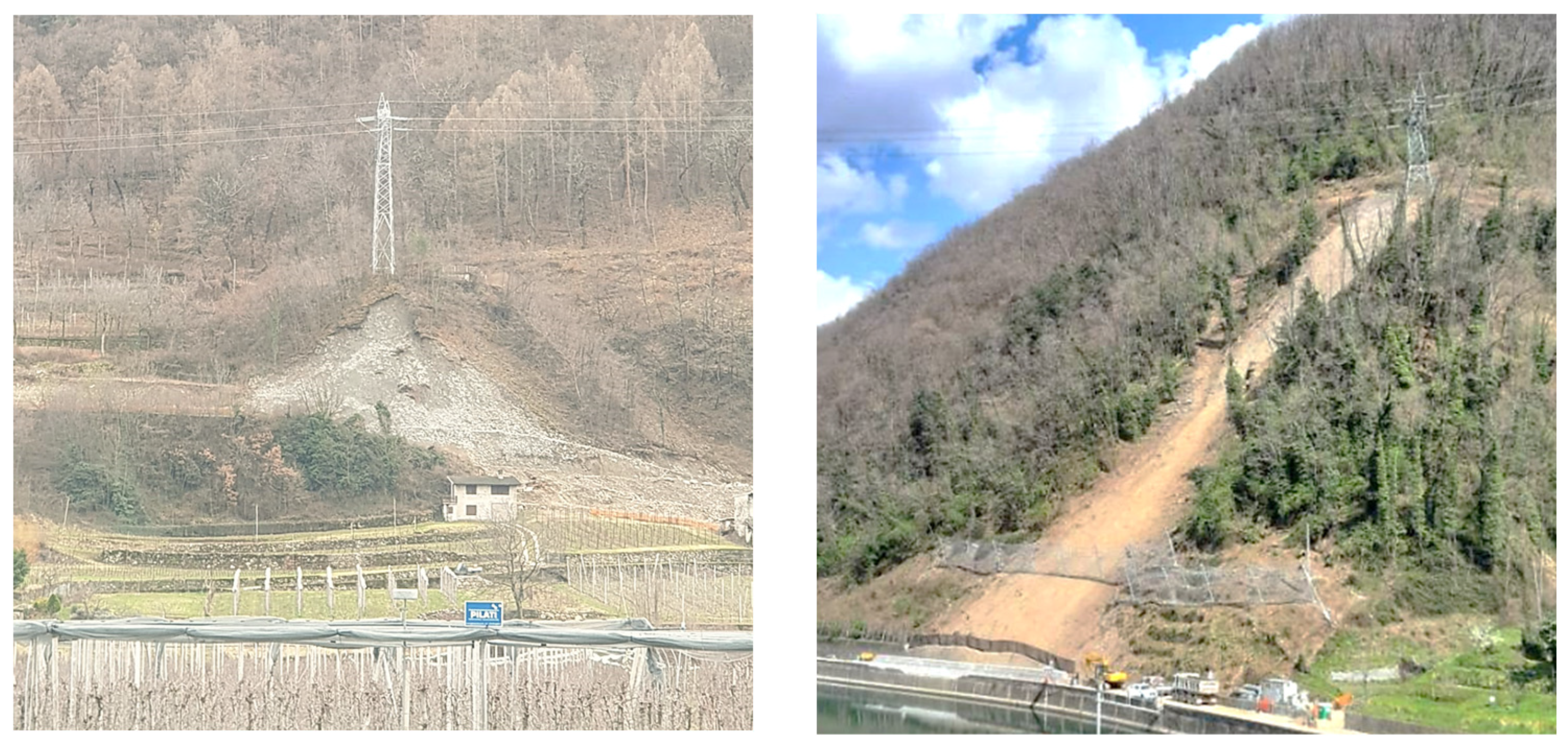
Considering these datasets, Italian Civil Protection has defined emergency plans that indicate the strategies to deal with the effects of geo-hazards at different regulation levels (municipalities, provinces, and regions) [8,22,23,24]. Following these indications, infrastructure stakeholders are starting to provide “resilience plans”. The former are documents where strategies against threats are involved in potentially increasing infrastructure resilience [25,26,27,28,29]. The partial failure of the electrical system may have a lot of repercussions on several sectors of human lives, especially during post-disaster emergency phases where power supply is a fundamental resource for local community recovery [22,30]. Geo-hydrological threats are, therefore, currently under investigation because they could seriously undermine the operativity and functionality of electro-energetic infrastructures [31,32,33], as highlighted by several episodes recorded in the past across Italian territory [2,15,16,34]. Severe floods may affect the operativity of dams and reservoirs because they have a crucial role in balancing extreme hydrological conditions and protecting downstream areas [8,28,35,36]. On the other hand, powerlines and power plants may be hit by landslides, causing local infrastructure failures and blackouts that may propagate through the whole electrical network [27,37,38,39,40] (Figure 1). In particular, rainfall-induced shallow landslides have been reported to be a common and rather destructive threat to powerline pylons [27]. These types of landslides are characterized by shallow depth (up to 2 m, reaching the bedrock) but with a significant planimetric extension [41]. They are triggered by terrain saturation due to the rainfall infiltration processes [42] and include soil slips and earth flow, which, in the presence of large amounts of water (i.e., terrain saturation and overland flow), may evolve into debris flows [43].

Figure 1.
Powerlines affected by shallow landslides in their proximities: slope failure can trigger pylon collapse, causing blackouts.
Shallow landslides exhibit rapid kinematics and have a predominantly two-dimensional geometry, so it is possible to make simplifications for modelling their ignition and dynamics by adopting distributed models in which the three-dimensional component is neglected [23,42]. In the literature, some examples refer to the scheme of the infinitely extended slope [12,42,44,45] where landslide triggering is evaluated in function of meteorological and climate forcing, i.e., heavy rains. Among others, the SHALSTAB (SHALlow slope STABility) model from [46] computes the critical rainfall intensity able to perturb shallow groundwater recharge as a measure for relative shallow slope stability. This tool combines a steady-state hydrological model (a topographic wetness index [47]) with an infinite slope stability model and identifies conditionally stable areas by reconstructing a susceptibility map of the territory. This model has been implemented, revised and extended by other authors [48,49,50] trying to overcome its limitations regarding the steady-state hydrological model and including a more complete slope stability routine. However, these solutions have not always considered the influence of the terrain’s partial saturation conditions on slope stability which is a determinant for accurate failure prediction [51,52].
Frequency ratio methods are commonly used for assessing landslide susceptibility [53], and in the literature, there are several examples of applications [7,54,55,56,57]. In order to apply them, it is necessary to evaluate the probability of slope failure over the investigated area, which is not trivial in the absence of a detailed census [53,58]. Therefore, other strategies have been proposed to infer the probability of rainfall-induced landslides, starting from the analysis of the triggering precipitation intensities and evaluating their temporal frequency or their return period [2,43,59]. Under the hypothesis of iso-frequency among critical rainfall and slope failure is also possible to infer the magnitude of the landslide event [2,7,59,60,61,62]. Namely, a rare event has a greater magnitude with respect to a more frequent one. Event magnitude estimation is necessary for carrying out a proper risk assessment and for defining the best strategies for increasing infrastructure resilience [27]. This is particularly true under the projected future climate change scenario where extreme events intensification is expected with high confidence [32,63,64]. This topic is currently a research frontier where several authors have started to define new methodologies for hazard assessment looking at predisposing factors (i.e., local territory susceptibility) and triggering factors (i.e., intense rainfalls) [23,24,56,57,65,66,67,68,69].
Taking inspiration from these literature works, the following paragraphs will present a revisited formulation of the model proposed by Borga et al. and successively improved by Tarolli et al. [50,70,71] The goal of our analysis was to find, improve, test, and validate a tool able to estimate slope stability failure under different critical rainfall conditions across remote mountain areas where powerlines are generally located. This model was developed for shallow landslide hazard assessment, considering the role of precipitation (with a given duration d and intensity r) as the main triggering factor. The revised version is called SLEM (Shallow Landslide Express Model) and includes some parameterization novelties, bringing a Python-based automatization of the analysis. Compared with the spatially distributed models in which the hydrological cycle is reproduced in all its components, SLEM incorporates an expeditious methodology for fast geo-hydrological hazards assessment [3,8,72,73,74]. The need to adopt these types of models arose from the necessity to provide a more quantitative landslide hazard evaluation for planning purposes with respect to the classical qualitative landslide susceptibility models [30,57,75,76]. From a stakeholder’s viewpoint, a first approximation powerlines risk analysis represents a valuable propaedeutic activity to direct subsequent detailed investigations to the most hazardous areas.
In the following paragraphs, the analysis conducted with SLEM is presented. In Section 2, SLEM’s new features are presented, highlighting the modifications adopted. In Section 3, the powerline hazard assessment using SLEM applied to the case study of the Trebbia basin (Emilia-Romagna region, Italy) is presented. In Section 4, SLEM performances and limitations are commented referring to the risk analysis results while in Section 5, the main outcomes of the methodology are reassumed.
2. Materials and Methods
This paragraph presents the methodology proposed by [50,70,71], where an analytical solution for the critical rainfall triggering a shallow landslide failure is obtained by coupling a subsurface hydrological model with a slope stability model. Equation (1) shows the model proposed by Borga et al. [50] (derived from SHALSTAB) and then successively improved by Tarolli et al. [70,71]:
Within the square bracket are all the presented parameters related to the stability model of the infinitely extended slope, generally adopted for assessing rainfall-induced shallow landslide failures, as described by Iverson [42] and Harp [12]:
- ▪
- Cr and Cs: the cohesion of plant roots and soil [kPa] on vegetated terrain slopes;
- ▪
- ρw and ρs: the density of water and sediment under saturated conditions [kg/m3];
- ▪
- g, ht, and B: the acceleration of gravity (9.81 m/s2), depth of the ground [m], and contour length [m];
- ▪
- β and φ: slope and ground friction angle [°];
- ▪
- W: additional weight of plant biomass [kPa] on vegetated terrain slopes.
The innovative part of the model resides within the first three terms T, a(d), and rc(d), where hydrological quantities are combined as follows:
- ▪
- T: the transmissivity of the shallow soil [m2/s], obtained as a product of soil thickness ht for the saturated hydraulic permeability Ksat [m/s];
- ▪
- a(d): the Dynamic Contributing Area (DCA) [m2] of the upstream subsurface runoff, which can evolve (increase or decrease) depending on the rainfall duration d up to the maximum contributing area amax;
- ▪
- rcrit(d) is the critical intensity of precipitation [mm/h] of duration d that solves Equation (1).
In the next paragraph, the key passages described in [50,70,71] adopted to retrieve Equation (1) are reported. The hydrological model, the slope stability model and their coupling are reported in Section 2.1, Section 2.2 and Section 2.3. Then, the strategy adopted for evaluating DCA and for including initial soil moisture dependence is described in Section 2.4 and Section 2.5. In Section 2.6, the case study of the Emilia-Romagna region taken into consideration for the analysis is presented, while the description of the model implementation and initial data investigation is reported in Section 2.7.
2.1. Hydrological Model
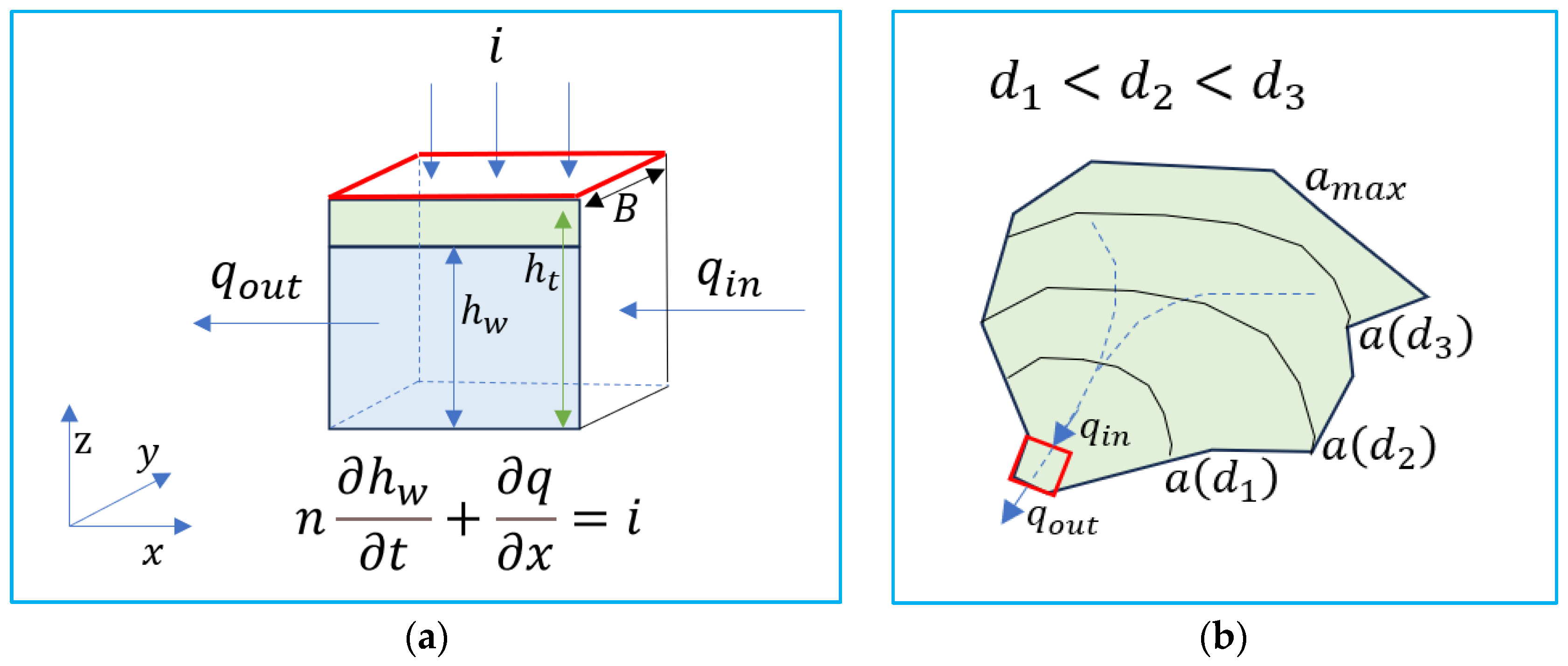
For assessing the hydrological model of the subsurface flow, the kinematic wave theory developed by [46,47,77] was considered. Starting from the continuity equation of the subsurface water flow (Equations (2) and (3)), the temporal variation of the effective soil water hw ∗ n [m] (where n is the terrain porosity [-]) depends on the advection term [m2/s] and the source term [m/s]. The first term describes the subsurface water flow variation along the slope element while the second represents the rainfall infiltration (Figure 2a). If the slopes are characterized by shallow soils, temporary aquifers may form after a period of rainfall. Considering the Dupuit approximation for the subsurface water flow velocity [50,78] (Equation (4), where hydraulic gradient is approximated by local terrain slope assuming the flow parallel to the bedrock), a stationary process (Equation (5), where ) and, integrating along the flow path coordinate x, the hydrological model reduces to Equation (6). In Equation (6), the quantity a represents the upslope contributing area for the subsurface flow while B is the width of the slope element (contour length) perpendicular to the subsurface flux. Neglecting any infiltration mechanism addressed to the rainfall rate (namely ) and assuming a constant rainfall rate , the soil water hw could be expressed as Equation (7). If the terrain slope β and the Ksat are constant and independent from time, the only quantity that could perturb hw depending on the rainfall duration d is the term a(d), the Dynamic Contributing Area (DCA) (Figure 2b).
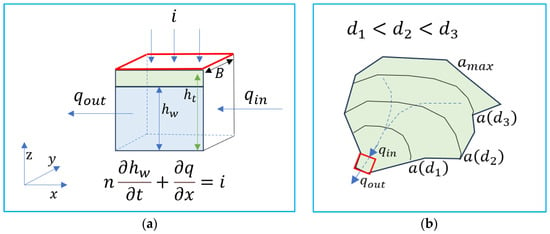
Figure 2.
(a) Continuity equation of the hydrological model according to [50,70,71], and (b) its exemplification at basin scale considering the Dynamic Contributing Area (DCA) a(d). The red box representes a single cell of the basin domain.
An analogue interpretation of this process was given by [46,48]. Their model divides a catchment into non-regular topographic elements defined by the intersection of elevation contours and orthogonal subsurface flow tubes. The rainfall completely infiltrates, forming shallow subsurface flow, which is routed downstream within the flow tubes. At any point on the slope and at any instant from the precipitation starts (d), the flow rate from the upstream portion of the basin is given by the product of the precipitation intensity ratio r0 (supposed constant) for the corresponding contributing area a(d) (Equation (8)). For water mass continuity, the inflow rate must be equal to the local downstream outflow which is regulated by Darcy’s law. Considering again the Dupuit approximation, the hydraulic gradient of the aquifer can be approximated by the tangent of the topographic slope β [47], giving the Equation (9). Under steady conditions, inflow and outflow equations could be merged by deriving the continuity equation of subsurface inflows-outflows (Equation (10)) that determines the fluctuation of the soil water height hw at a certain point along the slope. The hydrological model reduces similarly to Equation (7), where the dependence on rainfall duration d is again embedded in the term of a(d).
2.2. Slope Stability Model
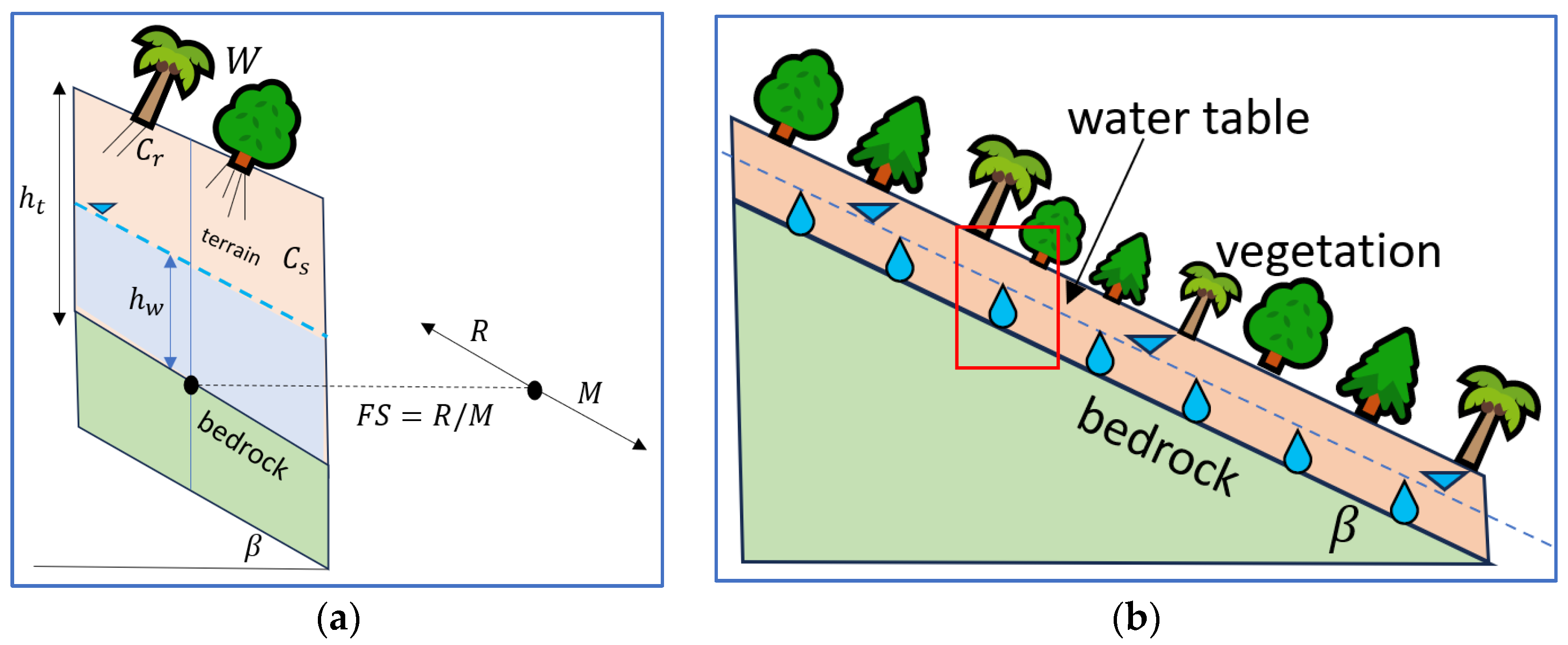
The second key part of the model described in Equation (1) is the slope stability equation for shallow landslide failure. Shallow landslides are distinguished from complex types such as roto-translational slips and gravitational slope deformations. For those types, the local geological component has a second-order effect with respect to the topography (slopes), and the geotechnical characteristics of the soil layers (angle of friction and cohesion) are responsible for their movement [12,42,44]. According to the literature [12,42,44,45,52,79], the most common approach to assess terrain stability follows the limit equilibrium equation applied on the infinite slope (Figure 3a). Here, each piece of terrain is subjected to mobilizing (M, in [N]) and resisting (R, in [N]) forces, which are derived by [50,70] for a cohesionless condition as reported in Equation (11). The factor of safety (FS) represents the ratio between R and M, and it is usually considered for assessing the slope stability conditions: if FS > 1, the slope is in safe conditions, while if FS < 1, a landslide may occur. By imposing the critical condition FS = 1 for the landslide ignitions, it is possible to determine explicitly the critical soil water height hw that can trigger the failure. The ratio among soil water and soil depth represents the critical soil moisture ratio Sr_crit, which depends on five parameters that are related to the terrain stability characteristics: soil and water densities, slope inclination and terrain friction angle .
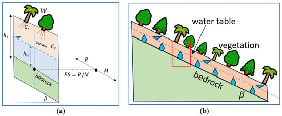
Figure 3.
(a) Continuity equation of the slope stability model according to [50,70,71], and (b) its exemplification at slope scale.
Following the work of [71], Equation (11) is reworked, adding two terms that are generally required for assessing slope stability for natural slopes: the cohesion and the vegetation surcharge [52,71] (Figure 3b). The cohesion represents the additional resistance given by the soil and tree roots and is a significant contribution to terrain stability, especially over steep slopes. Soil cohesion is generally comprised between 0–20 kPa [52], which could be neglected for coarse and sandy soils, while it tends to increase for clay soils. Tree root cohesion is related to the presence of forest above the slopes and is generally comprised between 0–10 kPa [52]. The presence of vegetation can also contribute to the stability through the surcharge W, which is consistent in a dense and mature forest up to values of 2–5 kPa [52]. The complete formulation shown in Equation (12) was considered under limit equilibrium FS = 1 for assessing the critical soil water content hw.
2.3. Coupling Hydrological Model with Slope Stability Model
Following the approach proposed by [50,70,71], starting from Equation (7) or (10) (the hydrological continuity equation), it is possible to combine with Equation (12) (the slope stability equation) under a few assumptions:
- ▪
- The rainfall duration dependency within rcrit(d) is assured only by the term a(d) (the DCA);
- ▪
- The critical rainfall rcrit able to trigger the failure is steady precipitation, neglecting possible intermittencies;
- ▪
- The transmissivity T is obtained as the product of Ksat and ht under the hypothesis of a free surface (not confined) aquifer formed within shallow soils.
Considering these statements, the value of the critical precipitation intensity could be explicitly derived by reworking Equation (14) to Equation (15), which is the same as Equation (1).
Equation (15) presents in a closed form a practical solution for rapidly quantifying the critical rainfall that is able to trigger slope instability, simply specifying the possible duration of that precipitation. This equation is similar to the SHALSTAB model except for the DCA term (which is not constant or equal to amax but it is dependent on d) and the additional terms of the shallow landslide stability model (Cs, Cr and W). Keeping the strength of this analytical and compact form, the application of Equation (15) for territorial susceptibility analysis should be carried out with care, bearing in mind the simplifications adopted for retrieving rcrit values:
- ▪
- The first one concerns the intensity of the critical rain rcrit, which is considered constant for a defined duration d. This hypothesis is unlikely when compared with the rainfall data collected by meteorological stations (rain is strongly intermittent [2,15]), but it is generally accepted for statistical analysis on extremes, such as the evaluation of the corresponding return time through the use of Intensity Duration Frequency curve (IDF) [80,81]. Using local valid IDF curves, the relation between critical precipitation intensity rcrit and the return time (TR) is uniquely determined. However, a shallow landslide is not a repetitive phenomenon that follows the cyclicity of precipitation, especially when investigated at the very local scale of the single slope portion [2,9,34,61,62,82]. Looking at the watershed basin scale, this assumption could be more accepted, admitting that adjacent areas may experience similar behaviour under the same triggering factors [52].
- ▪
- The second one concerns the determination of the contributing area a(d) as a function of time (namely rainfall duration d). As a precautionary measure, the contributing area could be considered as a constant that corresponds to the maximum upstream area amax at each point of the basin [50]. The contributing area can be evaluated in a fairly simple way using a GIS (Geographic Information System) software through the determination of flow accumulation [77,83]. However, this parameter may evolve with time because of the downstream propagation of subsurface water flow in the soil ground and across the basin so that it is a dynamic quantity and not a stationary one [84]. The authors [50,70,71] have assumed the stationary hypothesis with a = amax, not providing a unique analytical approach for expressing it as a function of d. To overcome this limitation, our study investigated this problem by proposing a closed formulation of the dynamic contributing area a(d) (DCA), recalling some similarities with surface hydrology, as presented in the next paragraph.
2.4. Determination of the Dynamic Contributing Area (DCA) for Subsurface Flow
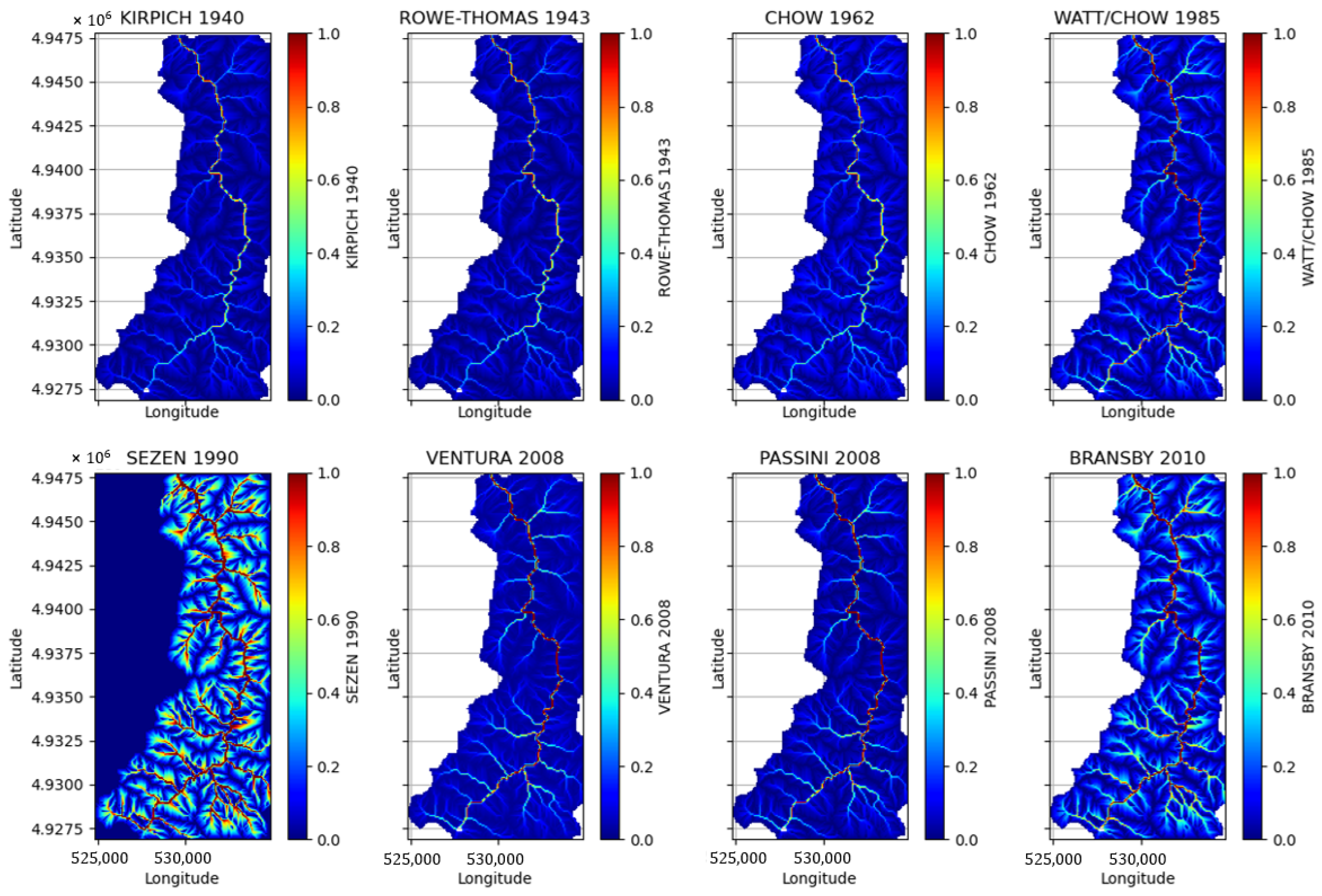
Within a catchment area, the time that a water drop takes to reach the closing section from any point of the basin is defined as the corrivation time Tc [72,85]. This parameter describes the average time with which superficial runoffs originate as a result of precipitation. Many formulas have been proposed in the literature for its evaluation as a function of the morphological and geometric parameters of the basin upstream of the closure point [85]. In this study, the formulas investigated were proposed by these authors [85]: Kirpich (1940), Rowe-Thomas (1943), Chow (1962), Watt-Chow (1985), Sezen (1990), Ventura (2008), Passini (2008), and Bransby (2010). The corrivation time is spatially variable and increases considerably along the main river reach and is reduced in the secondary branches and on the slopes (Figure 4). The Tc is a local property of the watershed basin [72]; therefore, the average value among the eight formulas investigated has been calculated for the entire domain to estimate a representative value of Tc.
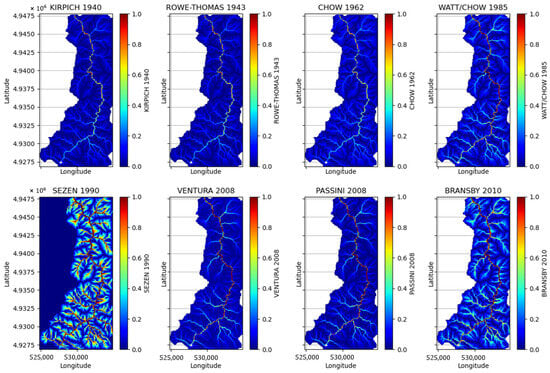
Figure 4.
Evaluation of surface corrivation time (normalized with respect to the maximum value of 1 h) using some formulas from the literature [85]: Kirpich 1940, Rowe-Thomas 1943, Chow 1962, Watt-Chow 1985, Sezen 1990, Ventura 2008, Passini 2008, and Bransby 2010.
The corrivation time can be interpreted as a time threshold when the entire area settled upstream of the considered closing point (amax) contributes to the outflow: for times less than Tc, the superficial contributing area asup(d) is <asup(Tc) = amax; for times greater than Tc, the superficial contributing area asup(d) = asup(Tc) = amax. Because the function asup(d) is strictly monotonic increasing, it is possible to model the growth curve using the time by a simple linear function (Equations (16) and (17)).
Generally speaking, the growth curve asup (d) should be determined uniquely for each river basin considering its geometric and geomorphological characteristics that, by definition, are not uniform [47,84]. More complex models for describing asup (d) fall outside the goal of making this methodology simple to apply straightforwardly. The method has been extended in a similar way considering the subsurface flow following the elaborations proposed by [49,86], evaluating a(d) as a function of the corrivation time of the subsurface flow Tc_sub (Equation (18)). This second case is one of interest for the application of SLEM, and the following considerations were taken into account:
- ▪
- The subsurface or hydrogeological basin is coincident with the hydrographic one (generally accepted if we consider surface layers lay on an impermeable crystalline substrate) [87];
- ▪
- The average saturated permeability Ksat of the surface terrain is variable across broad ranges, but for the loam soil type, which is one of the prevalent across the Italian landscape [88], a representative value may be around 10−5–10−6 m/s. Because the surface runoff velocity Vsup has an order of magnitude around 1 m/s, it is reasonable to increase the corrivation time of the subsurface flow Tc_sub as a function of the ratio of the two flow velocities (Equation (18)).
As a result, the term a(d) was determined by converting Tc into Tc_sub and applying Equations (19) and (20), giving a representation of the time variation of the DCA as a function of the kinematic and geomorphological parameters of the catchment. Implementing the DCA formulation of Equation (21) in Equation (15), the model dependency on Ksat could be discarded, at least for those areas where the condition is satisfied. Therefore, Equation (15) reduces to Equations (22) and (23), which represent the constitutive equations of the revised SLEM model.
2.5. Initial Soil Moisture Influence on DCA
The SLEM model does not explicitly consider the dependence on initial soil moisture because a complete saturation of the watershed basin is assumed. These conditions, although precautionary, are not representative of the partial saturation of the soils that, in many cases, guarantee their stability [41,71,73,74,75]. The terrain imbibition is time-dependent, and the complete saturation can only be reached in the long term and only for those areas morphologically predisposed to collect subsurface waters such as troughs and impluvium. In this regard, the condition of partial saturation of the slopes depending on soil moisture should be taken into consideration. Several authors [48,49,86] have proposed solutions to include the soil moisture dependency within the model. Taking inspiration from these analyses, the DCA parameter has been further reworked by including the relative permeability term Kr_ini for reducing the Ksat [89,90]. As reported in Equation (24), Kr_ini is non-linear dependent on initial soil moisture, and it is approximately 0 for very dry soils, while it tends to be 1 for saturated conditions. Through Equation (25), it is possible to correct Ksat simply by multiplying for Kr_ini and then using Ksat_ini to evaluate Tc_sub and a(d). The macro effect of partial saturation is a reduction of soil permeability, increasing the subsurface flow corrivation times and reducing for a fixed duration d the DCA term. This correction is analogous to the one implemented within the Soil Conservation Service—Curve Number method [72] where the antecedent soil imbibition is taken into account for setting infiltration fluxes.
where λ from [89]
As reported in Table 1, a soil moisture scale is specified with a “code” from 0 to 4 covering the VERY_DRY up to VERY_WET conditions for the initial soil moisture Sr_ini. In the next paragraphs, the simulations reported were conducted considering an intermediate initial condition for the soil moisture, corresponding to Sr_ini = 0.5.

Table 1.
Soil moisture scale adopted in the revised model.
2.6. Case Study Description
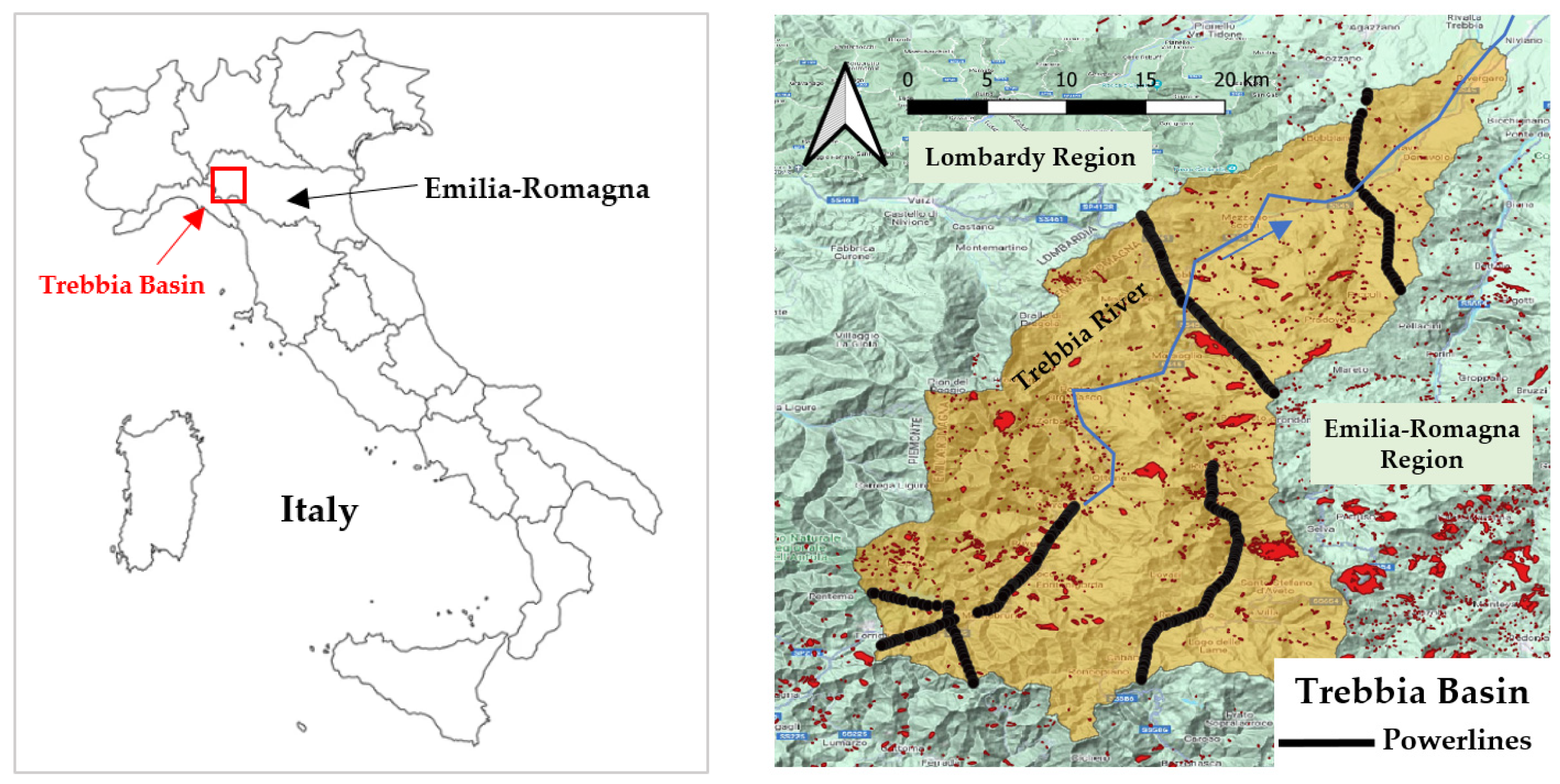
The SLEM has been tested across the Trebbia watershed basin, located in the northern part of the Apennines in the Emilia-Romagna region (Italy) (Figure 5). In the recent past, this catchment was hit by severe geo-hydrological issues (i.e., flash floods, debris flows, and diffuse landslide failures) triggered by heavy rain events. In October 2015, the Trebbia River was affected by a flood caused by a convective storm that triggered over the basin several episodes of shallow landslides and debris flow that hit main roads and town buildings and interrupted local infrastructures [65,66,91]. Across the Trebbia basin, several electrical infrastructures are exposed to geo-hydrological hazards because they are located in the proximities of landslide polygons mapped by the IFFI (Inventario Fenomeni Franosi Italiano) census [16] (Figure 5). In particular, due to their spread across impervious slopes, the high-voltage powerlines represent a vulnerable element of the regional electro-energetic network. The SLEM model was adopted to quantify the pylons at risk within the Trebbia basin using an automatized routine written in Python programming language.
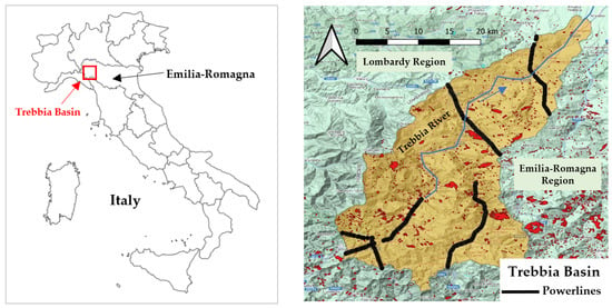
Figure 5.
Location of the case study conducted within the Trebbia watershed basin in Emilia-Romagna region (Italy). The high voltage powerlines settled across the basin are shown compared to the location of rainfall-induced landslides from the IFFI census (red polygons).
2.7. Python Scripts and Model Parameters Derivation
The model described in Equations (22) and (23) has been automatized to work with spatially distributed GIS data in raster format. The main goal was to create a set of “hazard maps” using the critical rainfall ratio rcrit varying the precipitation duration d. In this regard, four scripts written in Python language were created: 1_SOIL_Elaboration.py, 2_DCA_Elaboration.py, 3_SLEM_Model.py, and 4_TR_Evaluation.py.
- 1_SOIL_Elaboration.py:
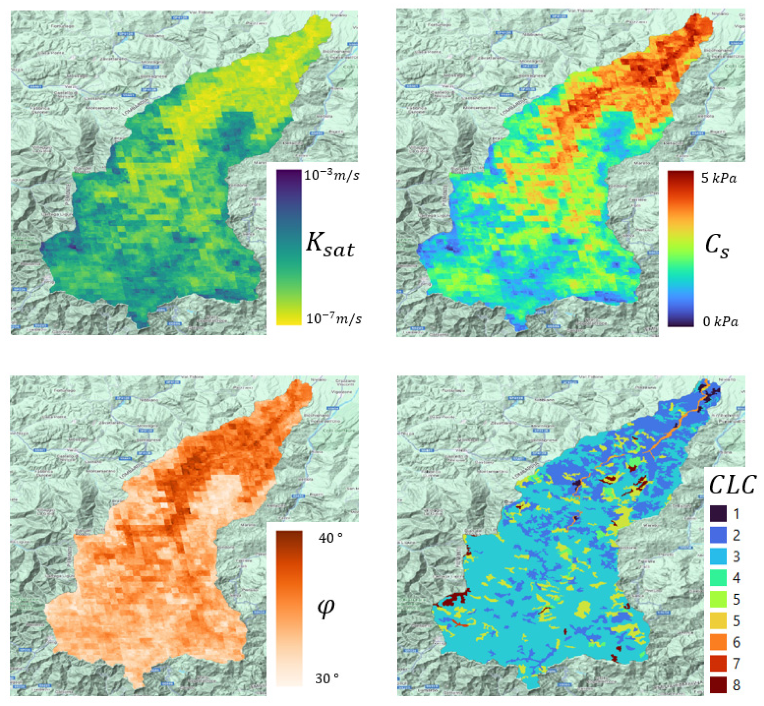
Preparatory processing of the soil data was carried out to evaluate the key parameters required for rcrit computation: the saturated permeability Ksat, the soil thickness ht, the friction angle φ, the soil and root cohesion Cs and Cr, and the vegetation surcharge W. Worldwide and national databases and literature studies [88,90,92,93] were investigated to retrieve these parameters for the investigated area, as depicted in Figure 6. More precisely, the Soil Grids database [88] was considered for retrieving soil texture distribution across the investigated area, assessing the % of fine (sand, silt, and clay) and coarse soils, and extracting the predicted shallow soil thickness ht. Conversely, Ksat distribution and unsaturated soil parameters were obtained from [89,90]. For friction angle and cohesion stability parameters, reference values and ranges [43,55] were considered for the main soil classes and then spatially distributed using the Soil Grids texture data. All the data were converted to a common raster format, “.map” [94].

Figure 6.
Representation of the soil parameters , soil cohesion , friction angle , and for the Trebbia watershed basin located in Emilia-Romagna region (Italy) using the databases provided by [88,90,92,93].
Biomass influence on soil stability was taken into account, including the root cohesion Cr and the vegetation surcharge according to [95,96]. Because these parameters are related to vegetation coverage, the Corine Land Cover () [93] map was included in the model to spatially distribute these quantities across the catchment. The contingency Table 2 reports the relation between some categories and the and values retrieved from the literature.

Table 2.
Representation of the root cohesion and the vegetation surcharge as a function of categories.
- 2_DCA_Elaboration.py:
All of the hydrological and geomorphological parameters needed are evaluated starting from the manipulations of the digital elevation model (DEM) called “dem.map”. The Python PCRaster [94] and PYSHED libraries [97] were used to carry out and speed up some operations on DEM:
- The HydroSHED DEM [92] was considered in this study. This DEM has a nominal spatial resolution of 90 m at the equator (~70 m at 45° latitude), and it has been conditioned (void-filled) and made hydrologically continuous to be easily implemented within hydrological and hydraulic models. Other high-resolution DEMs are advisable to improve computation performances, but accurate preprocessing is recommended;
- Using PCRaster and PYSHED libraries [94,97], the flow direction, the flow accumulation and the slope and slope accumulation are calculated. These data are required for computing the river network and the relative distance to the river of each cell of the domain;
- Considering the formulae listed in [85] and the computed hydrological data, the surface corrivation time Tc is calculated, and the subsurface corrivation time Tc_sub is calculated using the approximations described by Equation (18) (Figure 7).
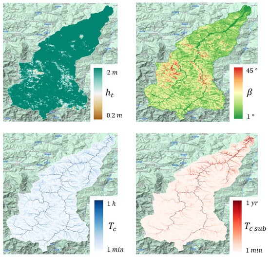 Figure 7. Representation of the soil thickness ht, slope angle , superficial corrivation time Tc, and the subsurface corrivation time Tc_sub for the Trebbia watershed basin located in Emilia-Romagna region (Italy) obtained from the HydroSHED DEM and [85].
- 3_SLEM_Model.py:
The script contains the implementation of the SLEM model shown in Equations (22) and (23), in which all the hydrogeological and stability parameters previously evaluated are ingested. The program evaluates the “hazard maps”, showing that the critical rainfall ratio rcrit is able to trigger slope failure for a series of reference rainfall durations, typically 1 h, 3 h, 6 h, 12 h, 24 h, 48 h, 72 h, and 120 h. For a fixed duration, the areas which admit lower rcrit are more prone to shallow landslide failure.
- 4_TR_Evaluation.py:
Following the applications made by [70,71], the return time of the critical precipitation (TR) is evaluated considering the rcrit and duration d in the function of the parameters a1, n, w, k, , and (Equations (26)–(28)) of the local IDF curves calculated using the Generalized Extreme Value (GEV) theory [80]. According to [2,7,9], the TR quantity is significant and represents a measure of the magnitude of the critical rainfall event, which is directly correlated to the shallow landslide magnitude. This is valid considering the hypothesis of iso-frequency among rainfalls and slope failures, which is generally accepted in the scientific literature, especially for explaining the recurrence of some rainfall-induced geo-hydrological phenomena such as flash floods and debris flow [7,9,43,72]. Namely, high rainfall return times correspond to lower probabilities of occurrence of landslides and vice-versa. The frequency-magnitude laws characterize geo-hydrological phenomena, so high TR also corresponds to significant landslide magnitude [7,9,98]. At the basin scale, the number of shallow landslides that occurred in the investigated area, their spatial density per km2 or their cumulative volume or area represent valid indexes for assessing a magnitude measure. According to [34,82], events of significant magnitude can present several landslides > 10 per km2.
3. Results
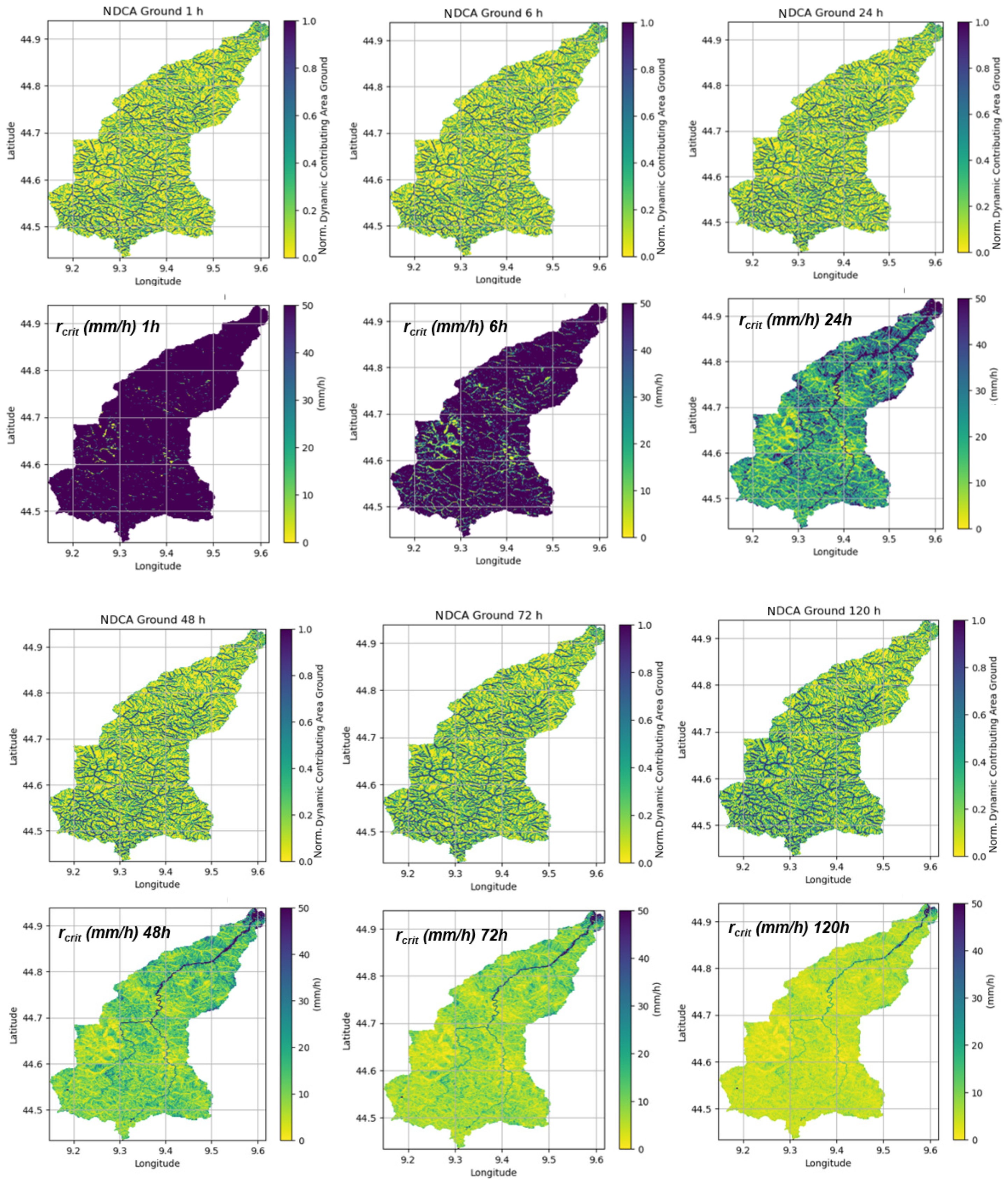
Figure 8 shows the Normalized Dynamic Contributing Area (NDCA = a(d)/amax, between 0–1) and the value of the critical precipitation intensity rcrit for durations of 1 h, 6 h, 24 h, 48 h, 72 h, and 120 h. As can be noticed, the NDCA obtained from DCA (Equation (19)) tends to progressively increase as the duration of the rain increases. Looking at Equations (22) and (23), the DCA term a(d) becomes predominant, increasing d, causing a reduction of the rcrit. Considering similar velocities of the subsurface flow, with increasing time, the NDCA tends to the maximum asymptotic value amax, following a monotonic function. In fact, if the picture of duration 1 h is compared with the one of duration 120 h, a drastic reduction of rcrit can be observed (from 50 mm/h to 5 mm/h, about 1 order of magnitude). This result has a physical meaning: increasing the duration of precipitation, watershed terrain tends to saturate, and the upper areas start to progressively contribute to the subsurface flow, reaching a regime condition when a(d) = amax.
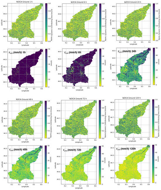
Figure 8.
Evaluation of the Normalized Dynamic Contributing Area (NDCA) and representation of the critical precipitation intensity rcrit, in mm/h, for increased rainfall durations: 1 h, 6 h, 24 h, 48 h, 72 h, and 120 h.
The power of the SLEM model consists of predicting not only when the failure may happen (i.e., the duration of the critical landslide triggering) but also individuating those areas where instabilities occur. Closely looking at the NDCA graph of Figure 8 with d = 1 h, only the slope areas placed at the ridges, where the saturated conditions are reached faster, are highlighted as critical. Gradually, these areas widen to the surrounding downstream slopes until, for a duration of 120 h, almost all the slopes, except the river, present a comparable lower rcrit. This result agrees with what has been observed in natural slopes where widespread shallow landslides often occur after prolonged rains that persist in an area for several days [99]. Conversely, if rain showers happen, only the steepest areas (the ridges) could experience localized instability, evolving sometimes into a debris flow [65].
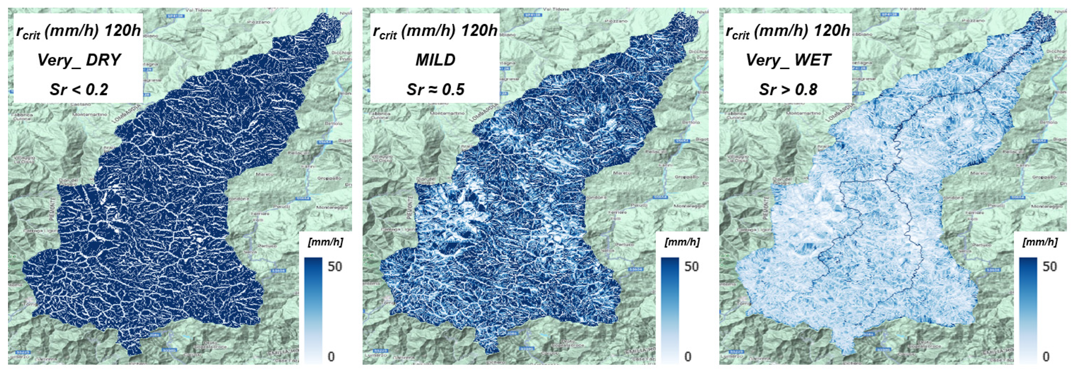
The influence of the initial soil moisture has been detected in rcrit results through a brief sensitivity analysis. Considering Table 1, SLEM was run under different soil moisture conditions from VERY_DRY to VERY_WET and for durations of 1 h, 6 h, 24 h, 48 h, 72 h, and 120 h. As can be appreciated from Figure 9, progressively increasing the soil moisture means a visible reduction of rcrit. This decrease is not uniform across the landscape, and it depends on the duration of the critical precipitation. On average, the rcrit reduction from a VERY_DRY to a VERY_WET condition is around 90% for a short duration (d < 6 h), while for long-lasting rainfalls (d > 24 h), the decrease is around 50%. The SLEM model is, therefore, rather sensible to the Sr_ini parameter. The areas with medium slopes (comprised between 20° and 40°, close to the typical soil friction angle values) are those that experience the main variation of the stability condition. These results are in accordance with geological and geotechnical studies [42,43,52,55,72], which predict soil moisture as one of the main drivers of natural slope stabilities.

Figure 9.
Representation of the critical precipitation intensity rcrit, in mm/h, for increased initial soil moisture condition for rainfall duration of 120 h. A reduction of rcrit is visible due to increased soil moisture.
3.1. Determination of the Return Time of the rcrit
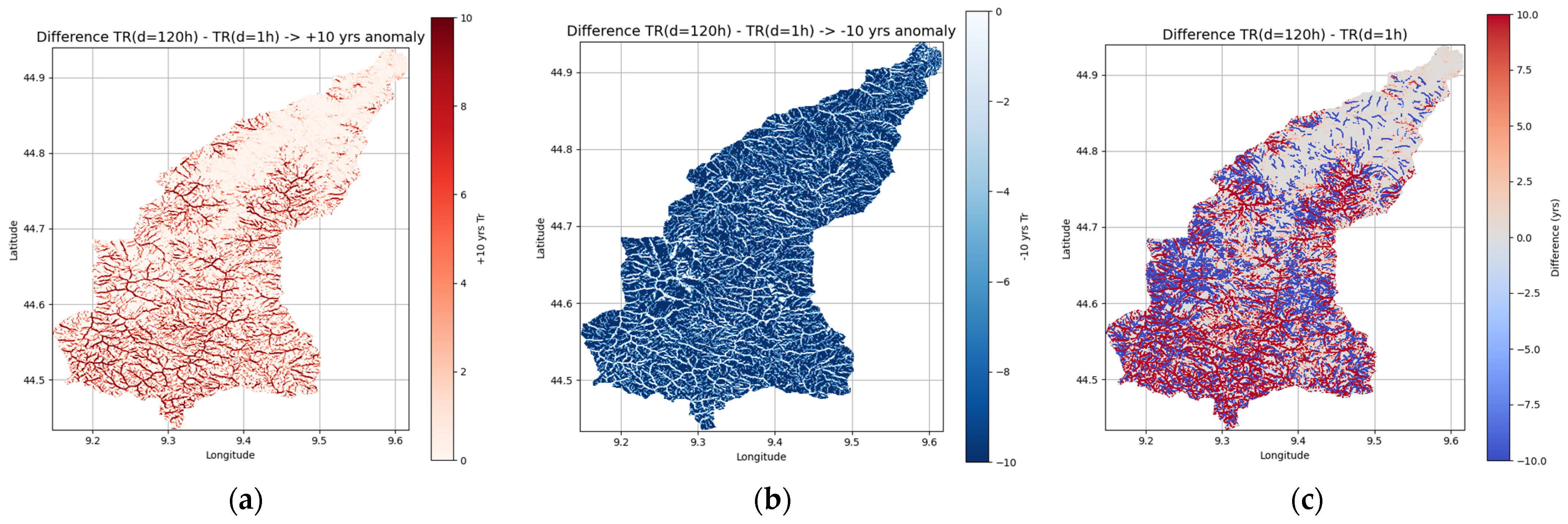
Once the value of the critical rainfall intensity has been obtained, the return time (TR) of that rain was evaluated using the IDF curves available for the Trebbia River basin [100,101]. The TR of precipitation represents an indirect estimate of the magnitude of the expected landslide phenomenon [2]. Using local IDF parameters listed in Table 3, the TR was assessed from the critical intensity rcrit and duration d pairs to retrieve information about the event magnitude. Six maps were obtained for the duration of 1 h, 6 h, 24 h, 48 h, 72 h, and 120 h. Then, to estimate the variation of the expected critical TR with the duration d of the precipitation, the difference between the TR maps relative to 120 h (“long-lasting rain”) and to 1 h (“short rain”) was carried out.

Table 3.
Parameters of the IDF considered for return time TR evaluation in the Trebbia River basin, from [100].
Figure 10 shows the variation in the critical TR for landslide triggering as a function of precipitation duration d. In red (Figure 10a) are the highlighted areas where the return time of critical rain rate rcrit is greater for prolonged rain (120 h) than for short rain (1 h). In blue (Figure 10b) are the highlighted areas where the return time of critical rain is lower for prolonged rain (120 h) than for short rain (1 h). The TR anomaly was evaluated in a range scale of ± 10 years. The distribution of red areas compared to blue ones is distinguished as follows: the red areas (Figure 10a) show the mountain ridges characterized by high gradients and low values of the subsurface contributing area, which are highlighted as mostly susceptible to intense but short rains (TR1h < TR120h); the blue areas (Figure 10b) highlight slopes characterized by lower gradients and higher values of the subsurface contributing area (TR120h < TR1h); the grey areas (Figure 10c) are those in which there is not such a significant tendency to vary the return time of critical rain as a function of duration (TR1h ≈ TR120h).
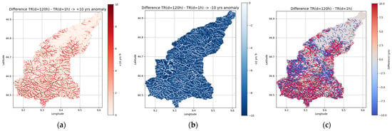
Figure 10.
Spatial variation of the critical TR with respect to the duration of precipitation in the Trebbia River basin. The maps are obtained by evaluating the difference between the TR for a duration of 120 h (long events) and a duration of 1 h (short events). The red areas (a) are those for which short events have lower TR than longer ones (TR1h < TR120h). The blue areas (b) are those for which persistent events have lower TR than shorter ones (TR120h < TR1h). The third figure (c) shows the combination of the two previous maps where the grey areas show a non-significant variation in the TR as a function of the rainfall duration.
Considering the frequency-magnitude theory [2], the most destructive shallow landslide episodes are expected from rainfall events with larger TR. These rare and catastrophic events have a relatively low frequency. However, from a probabilistic hazard perspective, electro-energetic stakeholders are interested mainly in coping with high-frequency failures because possible power outage needs to be reduced to the minimum during non-extreme events [27]. Therefore, for ridges, short and intense rains such as showers or thunderstorms represent the most hazardous trigger (TR1h < TR120h), while for slopes, these are represented by prolonged and low-intense precipitation (TR120h < TR1h). These results are confirmed by historical surveys [15,99] and could be explained in these terms: intense and short rains can saturate of faster the thin soil covers across ridge areas while prolonged rains can have a greater impact on the local hydrogeology, which contributes significantly to progressive (but slower) terrain saturation of the terrain slope over time. According to [46,47,50,78], this dynamic is directly imputed to the characteristic of the hydrological model chosen for simulating subsurface flow.
3.2. Threshold Curves Comparison for a Quantitative Validation of the Model
The SLEM model has been compared against the local rainfall threshold curves to address its reliability in predicting terrain failures for rainfall duration d. Rainfall thresholds (Equation (29)) are commonly used for determining the critical condition for shallow landslide collapse, simply considering only the rainfall as a trigger, i.e., the precipitation intensity and the duration [59,67,102] through empirical coefficients athrs and nthrs. Recently, in the Emilia area, there were several curves published [24,65,103] and, among them, we chose the most representative ones to validate the proposed model (Table 4).

Table 4.
Threshold curves were considered for the validation.
The Ceriani curve was developed in 1994, and it is generally adopted for the Lombardy region [102], which is located on the border of the Trebbia basin (Figure 5). This curve was considered one of the most affordable and representative for rainfall-induced phenomena such as debris flow and soil slips because it was retrieved from a quite large database containing several episodes that occurred across the Italian Alpine environment [103]. However, from a geological and lithological point of view, the Apennines and Alpine have different characteristics, so other authors (Segoni [24] and Ciccarese [65]) have reported the rainfall thresholds valid for the Northern Apennines. Segoni has established a threshold considering some critical rainfall events that occurred across the Emilia and Tuscany regions, while Ciccarese has defined two thresholds starting from two heavy rainfall events that occurred in the Emilia area in 2014 and 2015. The parameter athrs of Segoni and Ciccarese_1 threshold is very close to the Ceriani one while the nthrs parameter differs by about ±20%. On the other hand, Ciccarese_2 is higher than the previous and represents a sort of upper limit threshold where, according to the author, the probability of having a shallow landslide triggering after rain episodes above the threshold is almost certain.
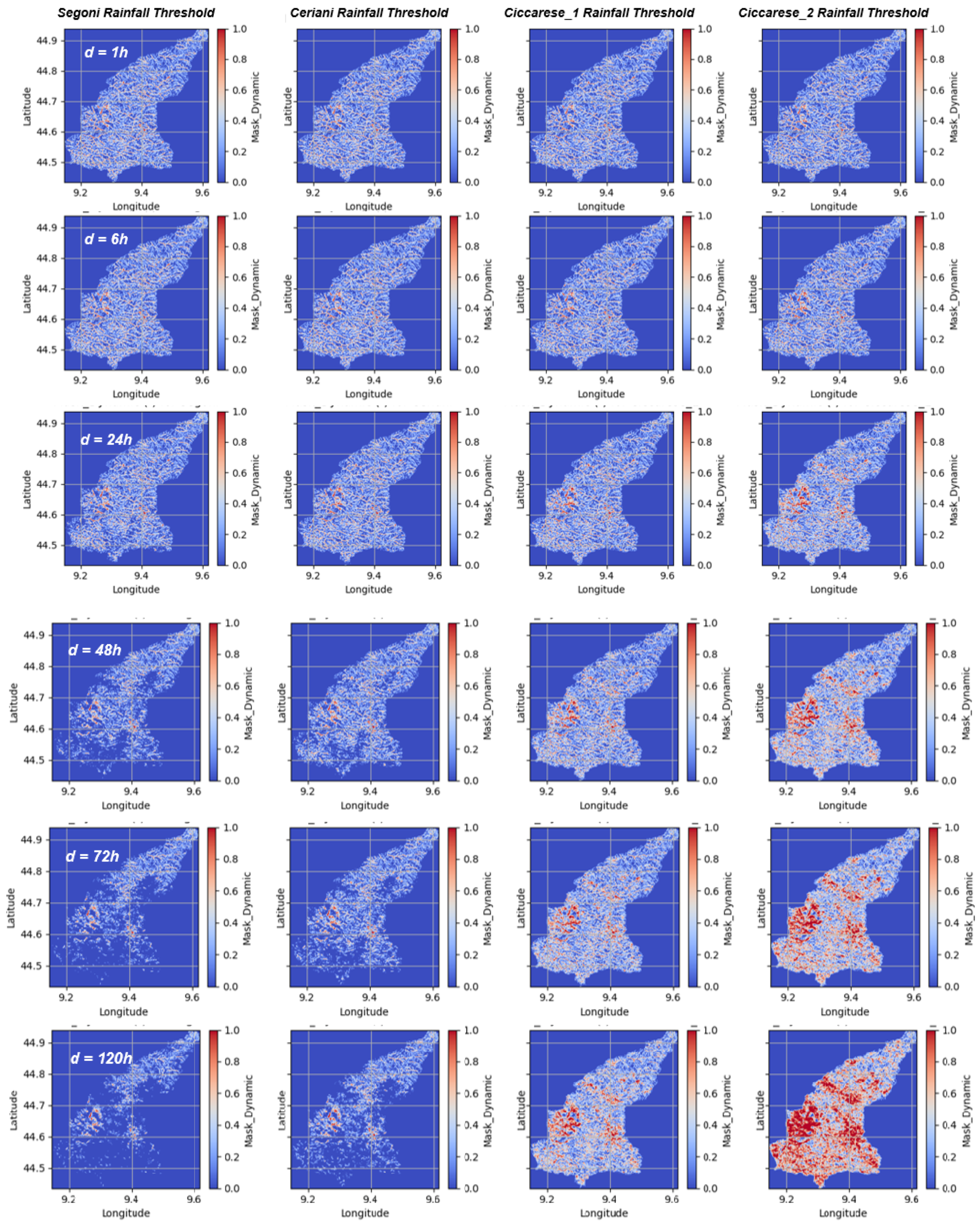
The validation of the model against the local threshold curves has been carried out through the MaskDynamic index and its combinations defined by Equations (30)–(32). In Figure 11, the MaskDynamic index calculation is reported for different rainfall durations d and is interpreted as follows:
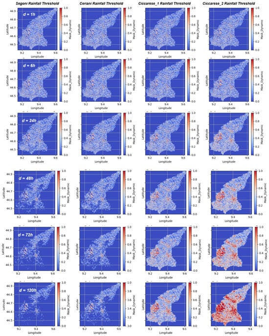
Figure 11.
Graphical representation of the MaskDynamic index for SLEM validation with respect to the local threshold curves of Segoni, Ceriani, and Ciccarese and for different durations of 1 h, 6 h, 24 h, 48 h, 72 h, and 120 h.
- ▪
- The index value is 0 (blue) when the critical rainfall for slope instability rcrit is equal to or above the correspondent rainfall threshold intensity;
- ▪
- The index value is 1 (red) when the calculated critical rainfall rcrit is settled below the threshold curve.
From the MaskDynamic index, the number of False Alarms (FA) and the Correct Predictions (CP) detected by the model can be derived. According to [104], FA and CP correspond to the FN (False Negative) and the TP (True Positive) indexes in the ROC (Receiver Operating Characteristic) methodology, respectively [105]. The latter is frequently adopted for assessing the performances of binary classification, such as the slope stability models that evaluate failure and non-failure conditions. The ROC methodology is completed if the other two categories (TN True Negative and FP False Positive) are also determined. However, for the SLEM model, imposing the limit equilibrium condition (which admits that failure surely happens) can reduce the ROC assessment, posing TN = FP = 0. In other words, the possibility that the model predicts a no-failure condition is neglected. The performance of SLEM was assessed both from graphical inspection (Figure 11) and using ROC performance indexes.
Looking at the four thresholds examined in Figure 11, it can be appreciated that Segoni and Ceriani behave quite similarly, varying the critical rainfall duration d. For short but intense rainfalls, SLEM gives rcrit below these thresholds, especially across ridges where high topographic gradients and fast hydrology can perturb the terrain stability faster. Here, the dynamic contributing area can reach its maximum value in a relatively short time (due to lower subsurface corrivation times), and steep slopes contribute to reducing the rcrit, which are settled below the rainfall thresholds. Similar behaviour is confirmed by other rainfall thresholds proposed by Ciccarese.
Conversely, for long-lasting events, the rcrit evaluated by SLEM has performed differently depending on the threshold chosen. For Segoni and Ceriani thresholds, the model performed less conservatively, giving rcrit above them. On the other hand, Ciccarese’s thresholds behave quite differently, especially for long-duration events (>48 h), showing a large number of areas where rcrit is settled significantly below (red areas). This is particularly true for Ciccarese_2, which is a higher threshold if compared with the others (Table 3). These results were partially expected because, according to the author [65], these thresholds best fit intense events that have triggered shallow landslides in a few hours or at least 1 or 2 days.
From the graphical analysis was noticed that that SLEM is rather in accordance with the Ceriani and Segoni rainfall thresholds, which represent the suggested curves for that area. However, our analysis has highlighted how their variability is not negligible, so SLEM performance may be affected depending on the threshold choice. To overcome this fact, the ROC analysis was conducted. According to [67,106], a rainfall threshold is determined by admitting a probability of 5–10% that a real landslide could not be detected by thresholds. In other words, there is a probability of 5–10% that a critical rainfall for triggering failure is settled below the threshold. This concept is inherited from statistical analysis and represents the probability of rejecting the null hypothesis that states that the threshold proposed is corrected for classifying critical and non-critical events in that specific area. Following this idea, that probability could be easily calculated using the performance index FAlr (False Alarms Rate) expressed in Equation (33). Conversely, the PPow (Predictive Power) of the model is calculated using Equation (34). To validate SLEM was our interest to try to verify the FAlr within the acceptable range of 5–10%.
As can be appreciated from Figure 12, the FAlr is around the value of 10% but tends to vary increasing the rainfall duration. In particular, the model prediction becomes worse if Ciccarese thresholds are considered for validation, rising FAlr up to 20–25% for d > 72 h. On the contrary, using Ceriani and Segoni thresholds FAlr reduces sensibly to values around 5%. The same consideration can be appreciated using the PPow index, which is higher for Segoni and Ceriani thresholds and lower for Ciccarese thresholds. Keeping the current parameterization, the SLEM validation is retained valid considering Segoni and Ceriani thresholds, confirming the results of the graphical analysis. SLEM validation against threshold curves permits to assessment of the reliability of the predicted instability in function of the critical rainfall, precisely describing local slope behaviour. According to [50], threshold curves inform about the predisposition of the area to trigger shallow landslides, while SLEM could zoom into the physical behaviour of the process, highlighting the location where critical situations may potentially occur.

Figure 12.
Performance assessment of SLEM showing the FAlr and PPow indexes with respect to the local threshold curves of Segoni, Ceriani, and Ciccarese and for different durations of 1 h, 6 h, 24 h, 48 h, 72 h, and 120 h.
3.3. Powerline Hazard Estimation
After model validation, two ways for assessing the powerline’s hazard across the Trebbia watershed were tested. The rainfall intensity rcrit is a key parameter for defining the powerline hazards because lower values correspond to areas where instabilities may occur with higher frequency. As a result, those areas that admit a lower critical rainfall ratio are the ones where a slope failure is much more probable to occur during slightly intense precipitation, so they are the most vulnerable from an infrastructure viewpoint [34]. Critical rainfall is, therefore, a quantitative indicator that could be considered to prioritize the maintenance or relocation of the most vulnerable pylon.
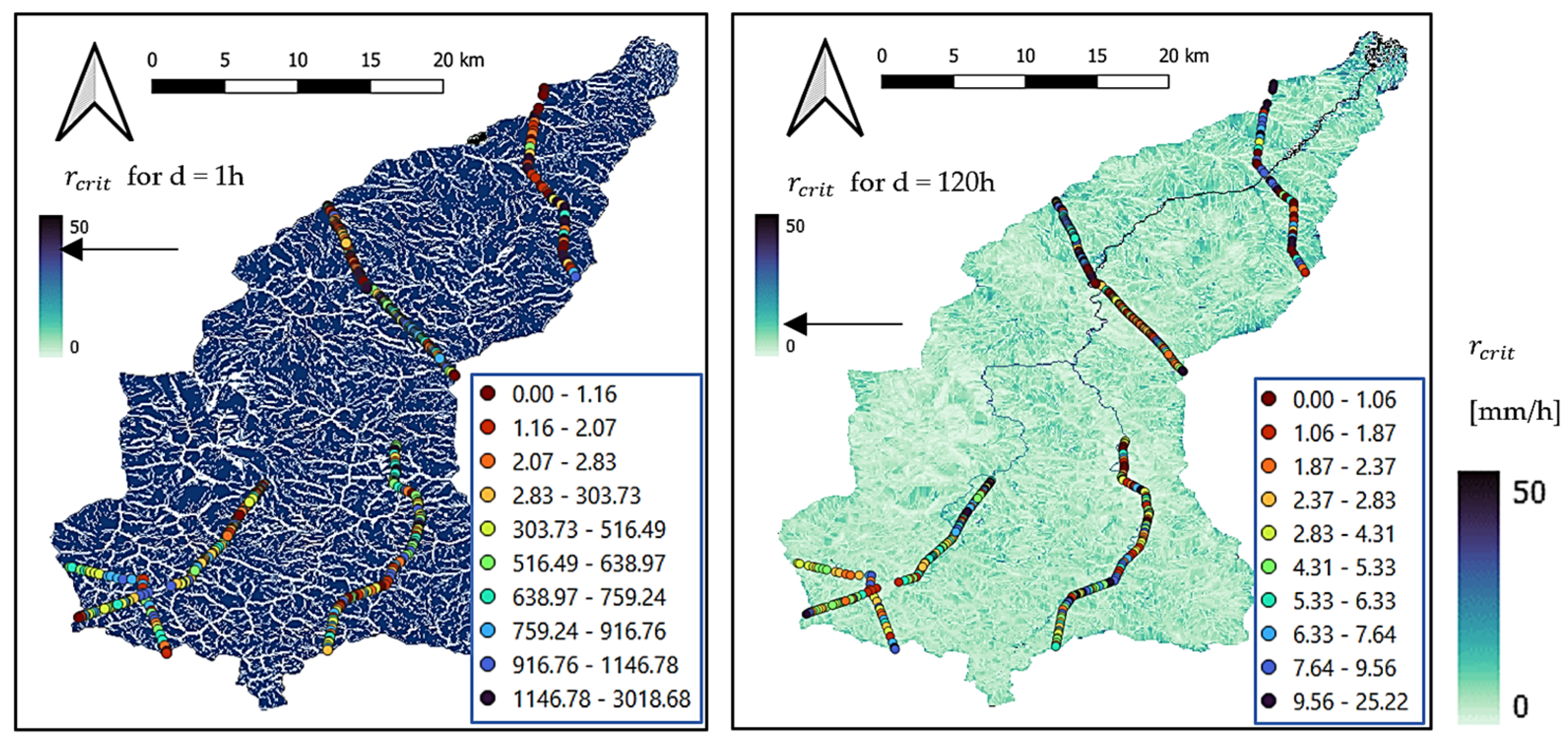
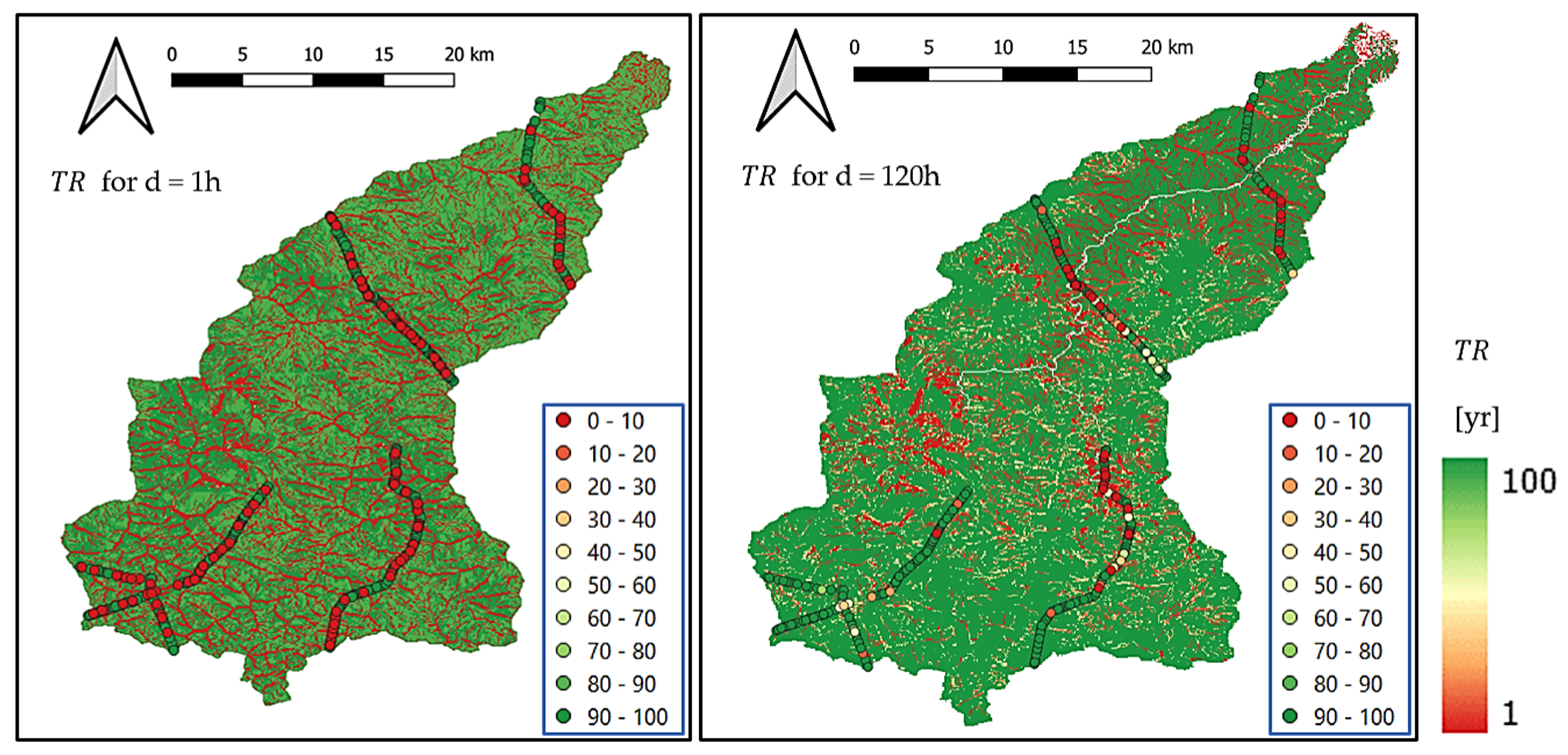
Different rainfall durations led to different critical intensities. Table 5 reports the statistics calculated for each pylon located in the Trebbia watershed (total number = 408). The mean rcrit is very high for low rainfall durations (<6 h) and tends to decrease to a more realistic value for higher d. Similar trends are confirmed by the variance. However, using rcrit is quite difficult to highlight the most vulnerable pylons simply comparing the maps shown in Figure 13, where rainfall durations of 1 h and 120 h are reported. Another possibility is to try to convert rcrit in terms of the TR of precipitation which is a measure of the temporal frequency of the critical rainfall event. In Equation (33), the critical TR period is assumed to be equal to the TR of the landslide failure (under the hypothesis of iso-frequency), which is equal to the TR of powerline failure if the landslide is triggered in the proximity of a pylon. Starting from these assumptions, the powerline failure could be directly related to the magnitude of the critical precipitation (Equation (35)), giving a better representation of critical areas across the Trebbia basin (Figure 14).

Table 5.
Statistics on rcrit for the 408 pylons located in Trebbia watershed basin.
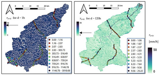
Figure 13.
Pylon ranking using the information of rcrit, expressed in mm/h and subdivided into 10 classes, for different rainfall durations (1 h and 120 h) located within the Trebbia watershed basin.

Figure 14.
Pylon ranking using the information of TR, expressed in yrs and subdivided into 10 classes, for different rainfall durations (1 h and 120 h) located within the Trebbia watershed basin.
As can be appreciated in Figure 14, different durations (d = 1 h and d = 120 h) led to different rcrit and TR of failure. To highlight this aspect in the map, red colours were selected for lower return time (i.e., more frequent landslide failure) and green colours for higher return time (i.e., less probable). Then, the TR was sampled in correspondence with the location of each powerline pylon, calculating some statistics reported in Table 6. By looking at the pylon points, mean TR varies with d within the range of 60–80 yr with a significant variability around 40 yr. The maps highlight those areas prone to failure for a short duration and intense precipitation, and others where failure occurs for long-lasting events.

Table 6.
Statistics on TR for the 408 pylons located in the Trebbia watershed basin.
Elaborating on the maps of Figure 13 and Figure 14, it is possible to extract the number of pylons at risk. A first extraction was carried out considering the pylons with rcrit values above the rainfall thresholds of Ceriani, Segoni, and Ciccarese. In Figure 15 it can be seen that for d = 1 h, the number of pylons detected at risk is 275, and the results computed for each threshold are in agreement. Conversely, for long-lasting events (d > 24 h), the results are quite variable: using the Ceriani and Segoni threshold, the number of the pylons at risk is projected to increase up to 350–360, while using the Ciccarese curves, the number of pylons at risk tends to reduce progressively to 200 or below. This technique strongly depends on the choice of the rainfall thresholds; therefore, the same analysis has been carried out using the TR quantity. Because slope failure recurrence is critical for assessing the infrastructure at risk, five classes of TR were defined in order to group rare and frequent events:

Figure 15.
Pylon statistics using the information of rcrit above the rainfall thresholds and TR evaluation for different rainfall durations (1 h and 120 h) located within the Trebbia watershed basin.
- ▪
- TR > 100 yrs, very rare;
- ▪
- 50 < TR < 100 yrs, rare;
- ▪
- 25 < TR < 50 yrs, fairly rare (range of the span life of powerlines);
- ▪
- 10 < TR < 25 yrs, frequent;
- ▪
- TR < 10 yrs, very frequent.
In Figure 15 the pylon classification in the function of the failure TR is presented. As can be noticed, this classification is dependent on the duration of the rainfall:
- ▪
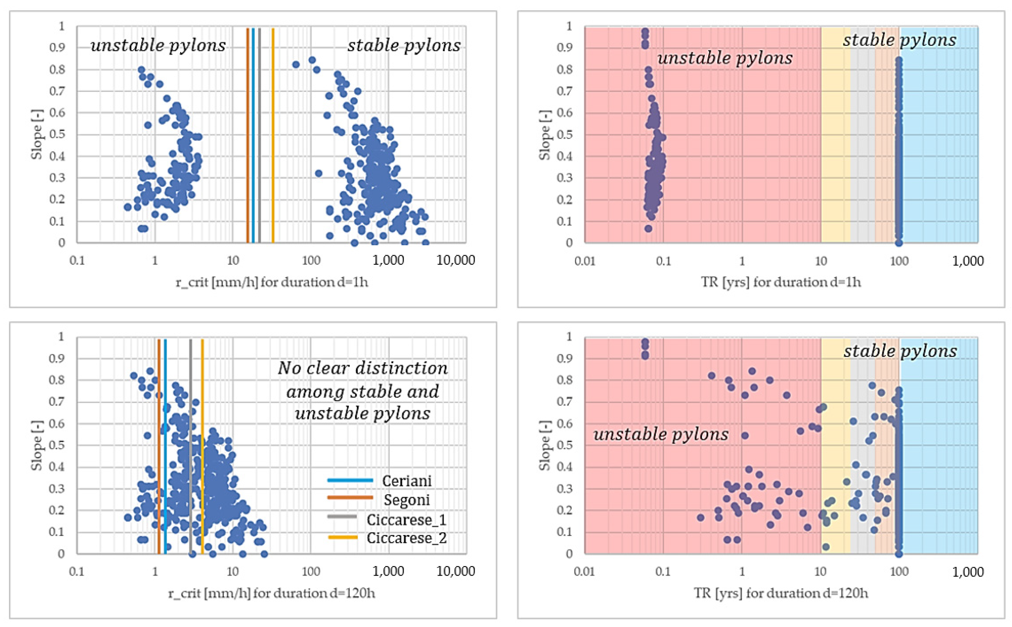
- For short but intense rainfall, the pylons are mainly classified into two groups, the stable pylons (where the failure is “rare”, around 270, 65% of the total) and the unstable pylons (where the failure is “very frequent”, around 130, 30% of the total). These clusters are also confirmed by Figure 16, where rcrit and TR were plotted against the topographical slope, which is a predisposing factor of slope instability. As can be appreciated, failure can happen at whatever slope inclination, but there is a consistent number of pylons that do not experience any instability.
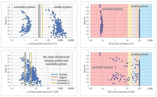 Figure 16. Pylon statistics using the information of rcrit and TR against the slope inclination predisposing factor evaluated for different rainfall durations (1 h and 120 h) located within the Trebbia watershed basin.
 - ▪
- For long-lasting precipitation (d > 24 h), the overall pylons at risk are reduced to 20–25% of the total, increasing the ones in safer conditions from 270 (d = 48 h) to 310 (d = 120 h). The pylons located in always unstable areas reduce to ~70–60 (around 15% of the total). The TR is more uniformly distributed for classes with TR < 100 yrs, showing a consistent reduction of the “very frequent” event (located across the ridges), while an increasing number of pylons within the “middle” TR classes is observed. Figure 16 also highlights how the rcrit is not able to distinguish safe and unsafe pylons, while with the TR data, stable pylons are clearly detected with respect to unstable ones.
4. Discussion
This work has presented an application of the SLEM model, firstly elaborated by Borga et al. and Tarolli et al. for evaluating the shallow landslide hazard and then reworked in this paper. The main purpose of the analysis was to evaluate the landslide hazard for some elements of the electrical network (powerlines). This represents a mandatory task required by electrical stakeholders for operational planning and for implementing resilience strategies to cope with these types of threats. The choice of this model has been driven by several motivations:
- ▪
- SLEM permits a faster simulation of the shallow landslide failure by simply merging an infinite slope stability model and a kinematic routing of subsurface flow. The parameters required are reduced to the minimum because it needs only information about topographical slopes, soil textures, and saturated permeabilities of shallow soils, which can be gathered from national and worldwide available databases. The parameterization of cohesion and friction angle coefficients is trickier, but it is possible to relate them to soil coverage and texture for retrieving a spatial distribution;
- ▪
- SLEM made explicit the relation between critical rainfall rate and slope stability through an approximate but physically consistent description of the hydrogeological water cycle. In fact, with respect to the classical simple slope stability model where each cell of DEM is considered independent of the other [12,42,44], the subsurface flow hydrological effect is quantified as a process that directly affects the stability of the terrain;
- ▪
- A sensitivity analysis was conducted to try to consider the perturbation of the initial soil moisture on the hydrological model included in SLEM. Taking inspiration from the works of [48,86], the soil moisture influence has been included within the DCA term. The former has been calculated as a function of Ksat_ini through the term Tc_sub, which could be expressed as a function Sr_ini. These dependencies were detected during the sensitivity analysis conducted in varying initial soil moisture conditions (as reported in Table 1), giving reasonable results that are in accordance with the literature studies [42,43,55];
- ▪
- The definition of the critical rainfall rate that triggers instability for a defined duration across a basin establishes the link between the cause and the effect and mimics the geo-hydrological interaction at the slope scale. In fact, for each point of the watershed (i.e., cell of the domain), the expected frequency of that critical rainfall could be estimated (i.e., return time). From TR, it is possible to measure the magnitude of the rainfall phenomena and consequently infer the magnitude of the geo-hydrological event and the probability of powerline failure;
- ▪
- The SLEM model represents an evolution of a well-established geo-hydrological routine that has been implemented in plenty of studies focusing on shallow landslide stability and susceptibility [46,48,49,50]. Its validation has been assessed in different case study areas of the world, considering one or a few reference rainfall events where a detailed slope failure census was available [48,70,71]. In our case, sufficiently precise data on past rainfall-induced slope failure events were not available, so the validation has been carried out following a statistical approach, adopting the locally available rainfall thresholds as a reference. To do that, the performance indexes inherited by ROC methodology were considered to assess the validation of SLEM, which has shown a slope failure detecting behaviour comparable to the rainfall thresholds indications. Implicitly, this procedure allows for sound model validity with respect to an ensemble of rainfall events previously considered for reconstructing the reference thresholds. In this way, the parameter calibration necessary to validate the model is not constrained to fit a single event but can be guided to match the typical statistical behaviour of the rainfall-induced landslides that happened in the past over the investigated area. This strategy allows to avoid parameter overfitting to a single-event analysis [43,55,72], increasing the robustness of the slope failure prediction. This procedure depends on how the threshold curve has been retrieved, but considering more than one threshold, possible discrepancies in reference curves could be detected easily, speeding up the model parameters calibration phase.
- ▪
- SLEM could be interpreted as an evolution of the rainfall threshold curves because it practically could detect through rcrit stability and instability situations at the level of a single DEM cell. This is a remarkable point because, using SLEM, the slope stability could be evaluated taking into account the local terrain susceptibility factors that, in rainfall threshold curves, are “hidden” within curves parameters athrs and nthrs;
- ▪
- In the end, the closed formulation proposed in Equations (22) and (23) permits the implementation of SLEM rather easily in Python language. The availability of PCRaster and PYSHED libraries has been considered to make hydrological elaborations faster. The flexibility of the code allows for the inclusion of further features, such as soil data elaboration and DCA calculation, by simply importing the required input data from external databases. Therefore, the SLEM equations scripting was rather fast and the sensitivity analysis for model calibration and validation was carried out quite rapidly.
4.1. Model Limitations
The SLEM model is a fast routine, and its mathematical construction is rather robust and validated by [49,70,71], but the application over areas should be carried out carefully, bearing in mind the assumptions and the input data uncertainties.
Regarding the hypothesis adopted in SLEM, the hydrological and slope stability models simplify the geo-hydrological interactions to make them computationally manageable and replicable. The definition of the parameter a (DCA) in the function of the rainfall duration d is a critical variable that has not been explicitly addressed by the authors of the model because it depends on several geo-hydrological processes related to subsurface water recirculation. DCA is an attempt to avoid the hydrological routing of subsurface flow which is a time-consuming operation but is fundamental for reconstructing subsurface dynamics across the watershed basin, influencing the local terrain soil moisture. However, the empirical laws describing corrivation time for surface flow may not be suitable for subsurface flow because hydrogeological watershed characteristics are different. This correction is valid under only in certain situations where the hydrogeological basin is supposed to coincide with the hydrological ones while the subsurface flow velocity is 10−5–10−6 lower than the surface according to saturated permeability. Moreover, the hypothesis that hydrological—hydrogeological basins overlap could not be acceptable in some cases, such as in the presence of karstic or multilayer aquifers [72]. In this light, the availability of local geological and lithological stratigraphy could represent an invaluable resource for better predicting the subsurface dynamics. These issues are currently investigated in complex geo-hydrological models and represent research frontiers [52].
Even though Sr_ini influence has been taken into account in the DCA term, some areas are barely dependent on the soil moisture and are detected as “unconditionally unstable” by SLEM. When DCA reaches its maximum value amax (i.e., all the areas of the basin contribute to the subsurface flow), the Sr_ini influence is missed. Here, the ratio T/DCA becomes a determinant for rcrit calculation. If all the rainfall r0 contributes to subsurface flow and a very low transmissivity is encountered locally, hw increases sensibly (from Equations (7) and (10)). Therefore, it may occur that hw could not resolve Equation (12) of the stability model, bringing FS << 1. Because the SLEM model requires FS = 1, the only possibility is to try to reduce hw by reducing the rainfall ratio r0. This represents a frequent condition encountered over watershed ridges, which are generally classified as unconditionally unstable areas by landslide susceptibilities models [24,56]. Over the ridges, SLEM predicts a rcrit ≈ 0 because steep slopes, thin soil depths, and low-contributing areas (where T ≈ DCA) bring FS < 1. According to [46,50], reworking on Equation (1) imposing r0 = 0 and neglecting the cohesion and surcharge terms, the limited condition for unconditionally unstable slope simplify and could be expressed as a function of soil and water densities (ρw and ρs), slope inclination β, and friction angle φ. This dynamic better explains Figure 9 where watershed ridges exhibit rcrit ≈ 0 also in VERY_DRY condition while intermediate slopes experience a larger influence on soil moisture variation. Because powerlines are frequently located over those impervious areas (Figure 5), further investigations are required to better disentangle predicted unstable areas from the effective landslide-prone areas. This fact has been highlighted in Figure 15 and Figure 16, where always unstable pylons (with rcrit ≈ 0 or TR < 10 yr) represent a consistent portion of the totals, especially for short rainfall durations. Performing the analysis with high-resolution DEM could be a good solution for increasing SLEM precision but checking the result with a local landslide susceptibility map is advisable to highlight the pylons under the highest landslide risk.
Because simple hydrological and slope stability models have been implemented in SLEM, the number of parameters required for critical rainfall assessment has been reduced to the minimum. This represents a valuable point because the scope of the analysis is to conduct a physically based survey sufficiently accurate for planning purposes. Apart from topographical data, which could be evaluated automatically using the DEM available, other soil parameters are more difficult to assess precisely. The literature datasets were preferred because they are easier to find on online repositories. Nevertheless, defining the most representative value inside the classes provided, often characterized by a broader range, and finding the most suitable methodology for spatially distributing the soil data properties are the main drawbacks. There is no standardized procedure due to the high spatial variability of soils across the landscape [88,90,107,108,109]. A methodology was proposed in this work to spatially extend the cohesion and friction angle information across the watershed. This procedure has already been adopted by other authors [72,110], especially for carrying out sensitivity analysis on soil infiltration parameters. However, this is an attempt to overcome the lack of spatially distributed data, which, for accurate slope stability computational analysis, should be estimated directly from geotechnical in situ surveys or laboratory experiments. Furthermore, a proper characterization using in situ measurement is sometimes not affordable, especially for the impervious area, which is the most prone to landslides. The methodology followed in this paper that tries to weigh each quantity in the function of soil texture may seem promising at least for a brief survey of slope stability for planning purposes, as the aim of our work.
The SLEM model was validated using the local rainfall threshold curves valid for the Trebbia basin. According to several authors [6,7,61,67], the reliability of those empirical relations is sometimes questionable because their calibrations strongly depend on the quality of the critical rainfall dataset. Uncertainties in rain gauge data estimations and the lack of rainfall peak detection may significantly perturb the rainfall threshold regression, leading to wrong interpretation of the triggering rain [104]. Fortunately, several studies have been conducted across the national territory in Italy that have the purpose to homogenise and standardize the rainfall threshold construction, reducing as much error as possible [67,102]. In this regard, the studies of Ceriani, Segoni, and Ciccarese represent one of the most recent analyses conducted in the investigated area, and those thresholds have been considered representative of the local Civil Protection planning. According to these authors, the uncertainties remain because, within the threshold curves, all the hydrological, geological, and geotechnical parameters that influence local slope stability are hidden. However, following the statistical interpretation of the curves, which are determined to allow a 5–10% probability of possible false alarm detection, the SLEM’s parameters were adjusted to address these standards. In our opinion, the local thresholds should be considered first to validate the model for understanding if the parameterization chosen is suitable or if a sensitivity analysis of parameters is required. Threshold curves represent a tool able to summarise the behaviour of an ensemble of critical rainfall events that happened over a region in the past. They show the typical rainfall–landslide empirical correlation, highlighting the peculiarity of the slope failure process across the investigated area, which should be ideally reproduced by more sophisticated spatially distributed models such as SLEM. In the case of the Trebbia basin, the model was rather in accordance with the local thresholds of Ceriani and Segoni, while for Ciccarese, the best accordance was acquired only for short-duration events. The choice of more than one threshold valid for the area is advisable for better model calibration.
4.2. Model Application to Assess Powerline Hazard
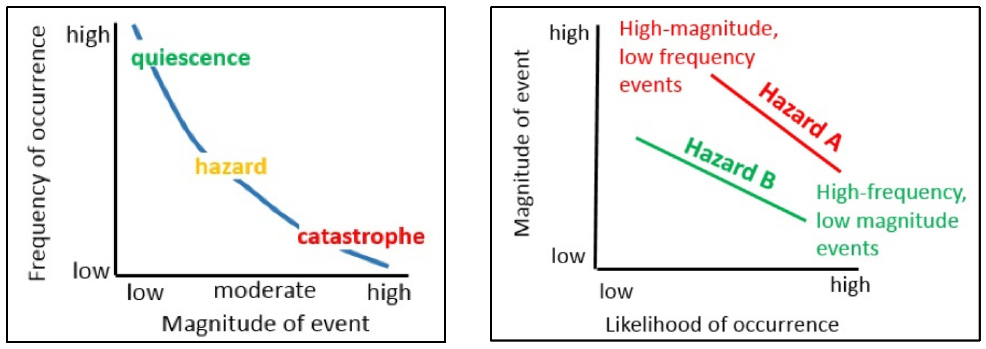
Thanks to its simplicity, SLEM has been applied to assessing powerline hazards. The latter has been described bearing in mind a correlation between the magnitude and frequency of occurrence (spatial or temporal) for natural phenomena and its relationship with respect to the event magnitude (Figure 17). For electro-energetic networks, both hazard frequency and magnitude and their relationship are interesting for future planning against geo-hydrological threats [27]. First of all, low TR episodes are critical because they can lead to instability rather frequently and increase the probability of electrical blackouts if pylons or stations are affected. However, because the magnitude of these events is expected to be low, periodic maintenance or mitigation strategies could be addressed more affordably to reduce the overall risk of failures. On the other side, high TR episodes are generally related to extreme precipitations whose effects at the watershed basin scale are difficult to predict accurately [2,111]. Extreme events may have catastrophic effects on the territory, triggering several geo-hydrological processes that cannot be completely described by the infinite slope model [10,67]. Because the magnitude of the correlated geo-hydrological event is expected to be higher, other types of risk reduction strategies should be analysed in order to cope with possible disasters. In these cases, pylon relocations seem to be the best cost-effective strategy to improve infrastructure resilience.
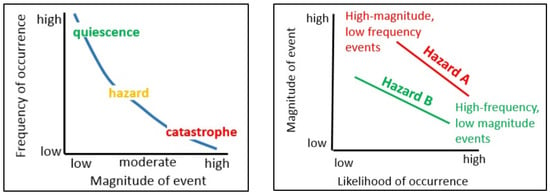
Figure 17.
Relationship between the probability of occurrence (spatial or temporal) and magnitude for natural events, from [112]: as the frequency of the phenomenon decreases, the expected magnitude increases and vice versa.
The maps reported in Figure 13 and Figure 14 clearly define these two possible scenarios that correspond to short but intense rainfall (left, 1 h duration) and long-lasting precipitation (right, 120 h). The most critical pylons coloured in red have a different distribution across the watershed in the two scenarios, and the subsequent elaboration reported in Figure 15 and Figure 16 confirms this fact. Some pylons are critical in both situations, while others are alternatively safer or not, depending on the duration of the critical precipitation. For short events, a clusterization among stable and unstable pylons can be clearly depicted, and this distinction mainly depends on their location in correspondence with watershed ridges. Conversely, for long-lasting events, the number of predicted unstable pylons is lower, but intermediate hazard situations may rise with failure return time comprised between 1 and 100 years, which is the range of the typical lifespan of electrical powerlines. Starting from these considerations, stakeholders could implement the most suitable strategies in terms of future maintenance and operational planning to improve the resilience of the overall electrical system against geo-hydrological hazards.
5. Conclusions
Strong uncertainties are linked to the modelling of geo-hydrological instability processes triggered by rainfalls, which pose some difficulties in evaluating those areas most prone to shallow landslides. The SLEM model examined in this study, although adopting important simplifications, represents an attempt to couple triggering factors (rainfall) and predisposing factors (terrain parameters) considering slope stability perturbed by water circulation in the subsoil. The parameters, compared to more complex models, are reduced to the minimum, making the methodology applicable, replicable, and suitable for geo-hydrological hazard assessment for planning purposes. SLEM is implemented within a Python code, which speeds up soil parameter reconstruction using available databases and repositories. The revised version implements a new methodology to evaluate the DCA parameter, which simplifies the model equation, excluding the dependence from Ksat and including the dependence on the initial soil moisture through Kr_ini.
Working at basin scale, it is possible to highlight the most critical areas that can cause slope instability as a function of precipitation of a given duration. The SLEM model was tested for the Trebbia watershed which in recent past experienced severe episodes of geo-hydrological instabilities. The model has been validated against locally available rain thresholds that represent a tool able to summarise the rainfall-induced landslide process using an ensemble of past precipitation events that occurred over a region. This strategy avoids model parameter overfitting to a single-event calibration, assuring the correct reproduction of the typical rainfall–landslide correlation existing over the investigated area. Considering the critical rainfall rate calculated, an evaluation of the return period is conducted to assess the magnitude of the event and to infer (under the hypothesis of iso-frequency) the magnitude of the geo-hydrological event. Superimposing the hazard maps onto the location of powerlines, a risk assessment was carried out for each pylon located within the Trebbia basin. The analysis has shown how the rainfall duration is a determinant factor for determining the most vulnerable infrastructures. The initial soil moisture increasing from dry to wet conditions causes a significant reduction of the critical precipitation rate between 50–90% depending on the rainfall duration. For short but intense rainfalls, around 30% of pylons are under failure risk, while for long-lasting events, the percentage reduces to 15–20%. Predicted failures are much more frequent across mountain ridges for short rainfalls, while landslide hazards are more uniformly spread during long-lasting events.
The risk analysis carried out with SLEM is intended for planning purposes because the model is able to highlight the triggering factors, the event magnitude, and the location where powerlines may be hit by geo-hydrological failures. Physically based hazard evaluations are the starting point for adopting possible mitigation strategies to increase the overall electro-energetic system resilience.
Author Contributions
Conceptualization, methodology, and validation, A.A. and L.M.; formal analysis, investigation, resources, and data curation, A.A.; writing—original draft preparation, A.A.; writing—review and editing, A.A. and L.M.; visualization and supervision, A.A. and L.M. All authors have read and agreed to the published version of the manuscript.
Funding
This work was financed by the Research Fund for the Italian Electrical System under the Three-Year Research Plan 2022–2024 (DM MITE n. 337, 15 September 2022) in compliance with the Decree of 16 April 2018.
Data Availability Statement
All the data provided and considered for calculations are available from databases and repositories cited in the texts. Python scripts and methodology, because they are under development and are frequently updated, can be directly requested from the authors at the address andrea.abbate@rse-web.it.
Conflicts of Interest
Andrea Abbate and Leonardo Mancusi were employed by RSE S.p.a. The authors declare that the research was conducted in the absence of any commercial or financial relationships that could be construed as a potential conflict of interest.
References
- Abbate, A.; Longoni, L.; Ivanov, V.I.; Papini, M. Wildfire Impacts on Slope Stability Triggering in Mountain Areas. Geosciences 2019, 9, 417. [Google Scholar] [CrossRef]
- Abbate, A.; Papini, M.; Longoni, L. Analysis of Meteorological Parameters Triggering Rainfall-Induced Landslide: A Review of 70 Years in Valtellina. Nat. Hazards Earth Syst. Sci. 2021, 21, 2041–2058. [Google Scholar] [CrossRef]
- Brambilla, D.; Papini, M.; Ivanov, V.I.; Bonaventura, L.; Abbate, A.; Longoni, L. Sediment Yield in Mountain Basins, Analysis, and Management: The SMART-SED Project. In Applied Geology: Approaches to Future Resource Management; De Maio, M., Tiwari, A.K., Eds.; Springer International Publishing: Cham, Switzerland, 2020; pp. 43–59. ISBN 978-3-030-43953-8. [Google Scholar]
- Longoni, L.; Ivanov, V.I.; Brambilla, D.; Radice, A.; Papini, M. Analysis of the Temporal and Spatial Scales of Soil Erosion and Transport in a Mountain Basin. Ital. J. Eng. Geol. Environ. 2016, 16, 17–30. [Google Scholar] [CrossRef]
- Ivanov, V.; Arosio, D.; Tresoldi, G.; Hojat, A.; Zanzi, L.; Papini, M.; Longoni, L. Investigation on the Role of Water for the Stability of Shallow Landslides-Insights from Experimental Tests. Water 2020, 12, 1203. [Google Scholar] [CrossRef]
- Guzzetti, F.; Peruccacci, S.; Rossi, M.; Stark, C.P. The Rainfall Intensity—Duration Control of Shallow Landslides and Debris Flows: An Update. Landslides 2008, 5, 3–17. [Google Scholar] [CrossRef]
- Corominas, J.; van Westen, C.; Frattini, P.; Cascini, L.; Malet, J.-P.; Fotopoulou, S.; Catani, F.; Van Den Eeckhaut, M.; Mavrouli, O.; Agliardi, F.; et al. Recommendations for the Quantitative Analysis of Landslide Risk. Bull. Eng. Geol. Environ. 2014, 73, 209–263. [Google Scholar] [CrossRef]
- Albano, R.; Mancusi, L.; Abbate, A. Improving Flood Risk Analysis for Effectively Supporting the Implementation of Flood Risk Management Plans: The Case Study of “Serio” Valley. Environ. Sci. Policy 2017, 75, 158–172. [Google Scholar] [CrossRef]
- Guzzetti, F.; Reichenbach, P.; Cardinali, M.; Galli, M.; Ardizzone, F. Probabilistic Landslide Hazard Assessment at the Basin Scale. Geomorphology 2005, 72, 272–299. [Google Scholar] [CrossRef]
- Rossi, M.; Guzzetti, F.; Salvati, P.; Donnini, M.; Napolitano, E.; Bianchi, C. A Predictive Model of Societal Landslide Risk in Italy. Earth-Sci. Rev. 2019, 196, 102849. [Google Scholar] [CrossRef]
- Fusco, F.; Abbate, A.; Calcaterra, D.; De Vita, P.; Guerriero, L.; Longoni, L.; Papini, M. Susceptibility Mapping of Shallow Landslides Inducing Debris Flows: A Comparison of Physics-Based Approaches. Ital. J. Eng. Geol. Environ. 2023, 1, 63–71. [Google Scholar] [CrossRef]
- Harp, E.L.; Michael, J.A.; Laprade, W.T. Shallow-Landslide Hazard Map of Seattle, Washington; Open-File Report: Reston, VA, USA, 2006; p. 23. [Google Scholar]
- Ozturk, U.; Tarakegn, Y.; Longoni, L.; Brambilla, D.; Papini, M.; Jensen, J. A Simplified Early-Warning System for Imminent Landslide Prediction Based on Failure Index Fragility Curves Developed through Numerical Analysis. Geomat. Nat. Hazards Risk 2015, 7, 1406–1425. [Google Scholar] [CrossRef]
- Quan Luna, B.; Blahůt, J.; Camera, C.; Westen, C.J.; Apuani, T.; Jetten, V.G.; Sterlacchini, S. Physically Based Dynamic Run-out Modelling for Quantitative Debris Flow Risk Assessment: A Case Study in Tresenda, Northern Italy. Environ. Earth Sci. 2013, 72, 645–661. [Google Scholar] [CrossRef]
- Luino, F.; De Graff, J.; Roccati, A.; Biddoccu, M.; Cirio, C.G.; Faccini, F.; Turconi, L. Eighty Years of Data Collected for the Determination of Rainfall Threshold Triggering Shallow Landslides and Mud-Debris Flows in the Alps. Water 2020, 12, 133. [Google Scholar] [CrossRef]
- ISPRA. Dissesto Idrogeologico in Italia: Pericolosità e Indicatori di Rischio; ISPRA: Ispra, Italy, 2018; ISBN 978-88-448-0901-0.
- ISPRA. Inventario Fenomeni Franosi. Available online: http://www.isprambiente.gov.it/it/progetti/suolo-e-territorio-1/iffi-inventario-dei-fenomeni-franosi-in-italia (accessed on 1 February 2024).
- Segoni, S.; Caleca, F. Definition of Environmental Indicators for a Fast Estimation of Landslide Risk at National Scale. Land 2021, 10, 621. [Google Scholar] [CrossRef]
- Gatto, A.; Clò, S.; Martellozzo, F.; Segoni, S. Tracking a Decade of Hydrogeological Emergencies in Italian Municipalities. Data 2023, 8, 151. [Google Scholar] [CrossRef]
- Jaedicke, C.; Van Den Eeckhaut, M.; Nadim, F.; Hervás, J.; Kalsnes, B.; Vangelsten, B.V.; Smith, J.T.; Tofani, V.; Ciurean, R.; Winter, M.G.; et al. Identification of Landslide Hazard and Risk ‘Hotspots’ in Europe. Bull. Eng. Geol. Environ. 2014, 73, 325–339. [Google Scholar] [CrossRef]
- Froude, M.J.; Petley, D.N. Global Fatal Landslide Occurrence from 2004 to 2016. Nat. Hazards Earth Syst. Sci. 2018, 18, 2161–2181. [Google Scholar] [CrossRef]
- Molinari, D.; Ballio, F.; Menoni, S. Modelling the Benefits of Flood Emergency Management Measures in Reducing Damages: A Case Study on Sondrio, Italy. Nat. Hazards Earth Syst. Sci. 2013, 13, 1913–1927. [Google Scholar] [CrossRef]
- Segoni, S.; Tofani, V.; Rosi, A.; Catani, F.; Casagli, N. Combination of Rainfall Thresholds and Susceptibility Maps for Dynamic Landslide Hazard Assessment at Regional Scale. Front. Earth Sci. 2018, 6, 85. [Google Scholar] [CrossRef]
- Segoni, S.; Lagomarsino, D.; Fanti, R.; Moretti, S.; Casagli, N. Integration of Rainfall Thresholds and Susceptibility Maps in the Emilia Romagna (Italy) Regional-Scale Landslide Warning System. Landslides 2015, 12, 773–785. [Google Scholar] [CrossRef]
- Vaagensmith, B.; McJunkin, T.; Vedros, K.; Reeves, J.; Wayment, J.; Boire, L.; Rieger, C.; Case, J. An Integrated Approach to Improving Power Grid Reliability: Merging of Probabilistic Risk Assessment with Resilience Metrics. In 2018 Resilience Week (RWS); IEEE: New York, NY, USA, 2018; pp. 139–146. [Google Scholar]
- Beyza, J.; Yusta, J.M. Integrated Risk Assessment for Robustness Evaluation and Resilience Optimisation of Power Systems after Cascading Failures. Energies 2021, 14, 2028. [Google Scholar] [CrossRef]
- Ciapessoni, E.; Cirio, D.; Pitto, A.; Mancusi, L.; Abbate, A. Modeling the vulnerability of power system components to debris flows for power systems resilience analyses. In Proceedings of the 2022 17th International Conference on Probabilistic Methods Applied to Power Systems (PMAPS), Manchester, UK, 12–15 June 2022; pp. 1–6. [Google Scholar]
- Fekete, A. Critical Infrastructure and Flood Resilience: Cascading Effects beyond Water. WIREs Water 2019, 6, e1370. [Google Scholar] [CrossRef]
- Xia, J.; Xu, F.; Huang, G. Research on Power Grid Resilience and Power Supply Restoration during Disasters-A Review. In Flood Impact Mitigation and Resilience Enhancement; Huang, G., Ed.; IntechOpen: Rijeka, Croatia, 2020; p. 8. ISBN 978-1-83962-626-5. [Google Scholar]
- Menoni, S.; Margottini, C. Inside Risk: A Strategy for Sustainable Risk Mitigation; Springer: Berlin/Heidelberg, Germany, 2011; ISBN 978-88-470-1841-9. [Google Scholar]
- Faggian, P. Climate Change Projection for Mediterranean Region with Focus over Alpine Region and Italy. JESE 2015, 4, 482–500. [Google Scholar] [CrossRef]
- Faggian, P. Future Precipitation Scenarios over Italy. Water 2021, 13, 1335. [Google Scholar] [CrossRef]
- Bonanno, R.; Lacavalla, M.; Sperati, S. A New High-Resolution Meteorological Reanalysis Italian Dataset: MERIDA. Q. J. R. Meteorol. Soc. 2019, 145, 1756–1779. [Google Scholar] [CrossRef]
- Trigila, A.; Iadanza, C.; Lastoria, B.; Bussettini, M.; Barbano, A. Dissesto Idrogeologico in Italia: Pericolosità e Indicatori di Rischio; ISPRA: Rome, Italy, 2021; ISBN 978-88-448-1085-6. [Google Scholar]
- Marnezy, A. Alpine Dams. From Hydroelectric Power to Artificial Snow. Rev. Géographie Alp. 2008, 96, 103–112. [Google Scholar] [CrossRef]
- ITCOLD. La Gestione Dell’interrimento dei Serbatoi Artificiali Italiani; Comitato Nazionale Italiano delle Grandi Dighe: Rome, Italy, 2009. [Google Scholar]
- Crosta, G.B.; Imposimato, S.; Roddeman, D.G. Numerical Modelling of Large Landslides Stability and Runout. Nat. Hazards Earth Syst. Sci. 2003, 3, 523–538. [Google Scholar] [CrossRef]
- D’Agostino, V.; Cesca, M.; Marchi, L. Field and Laboratory Investigations of Runout Distances of Debris Flows in the Dolomites (Eastern Italian Alps). Geomorphology 2010, 115, 294–304. [Google Scholar] [CrossRef]
- D’Agostino, V.; Marchi, L. Debris Flow Magnitude in the Eastern Italian Alps: Data Collection and Analysis. Phys. Chem. Earth Part C Sol. Terr. Planet. Sci. 2001, 26, 657–663. [Google Scholar] [CrossRef]
- Pereira, S.; Garcia, R.; Zêzere, J.; Oliveira, S.; Silva, M. Landslide Quantitative Risk Analysis of Buildings at the Municipal Scale Based on a Rainfall Triggering Scenario. Geomat. Nat. Hazards Risk 2017, 8, 624–648. [Google Scholar] [CrossRef]
- Varnes, D.J. Slope Movement Types and Processes. Spec. Rep. 1978, 176, 11–33. [Google Scholar]
- Iverson, R.M. Landslide Triggering by Rain Infiltration. Water Resour. Res. 2000, 36, 1897–1910. [Google Scholar] [CrossRef]
- Jakob, M.; Hungr, O. Debris-Flow Hazards and Related Phenomena; Springer: Berlin/Heidelberg, Germany, 2005. [Google Scholar]
- Milledge, D.G.; Bellugi, D.; McKean, J.A.; Densmore, A.L.; Dietrich, W.E. A Multidimensional Stability Model for Predicting Shallow Landslide Size and Shape across Landscapes. J. Geophys. Res. Earth Surf. 2014, 119, 2481–2504. [Google Scholar] [CrossRef] [PubMed]
- Montrasio, L. Stability Analysis of Soil-Slip. In Risk Analysis II; WIT Press: Billerica, MA, USA, 2008; Volume 45, pp. 357–366. [Google Scholar] [CrossRef]
- Montgomery, D.R.; Dietrich, W.E. A Physically Based Model for the Topographic Control on Shallow Landsliding. Water Resour. Res. 1994, 30, 1153–1171. [Google Scholar] [CrossRef]
- Beven, K.J.; Kirkby, M.J. A Physically Based, Variable Contributing Area Model of Basin Hydrology/Un Modèle à Base Physique de Zone d’appel Variable de l’hydrologie Du Bassin Versant. Hydrol. Sci. Bull. 1979, 24, 43–69. [Google Scholar] [CrossRef]
- Rosso, R.; Rulli, M.C.; Vannucchi, G. A Physically Based Model for the Hydrologic Control on Shallow Landsliding. Water Resour. Res. 2006, 42, W06410. [Google Scholar] [CrossRef]
- Lanni, C.; Borga, M.; Rigon, R.; Tarolli, P. Modelling Shallow Landslide Susceptibility by Means of a Subsurface Flow Path Connectivity Index and Estimates of Soil Depth Spatial Distribution. Hydrol. Earth Syst. Sci. 2012, 16, 3959–3971. [Google Scholar] [CrossRef]
- Borga, M.; Fontana, G.D.; Cazorzi, F. Analysis of Topographic and Climatic Control on Rainfall-Triggered Shallow Landsliding Using a Quasi-Dynamic Wetness Index. J. Hydrol. 2002, 268, 56–71. [Google Scholar] [CrossRef]
- Bao, H.; Liu, L.; Lan, H.; Peng, J.; Yan, C.; Tang, M.; Guo, G.; Zheng, H. Evolution of High-Filling Loess Slope under Long-Term Seasonal Fluctuation of Groundwater. CATENA 2024, 238, 107898. [Google Scholar] [CrossRef]
- Abbate, A.; Mancusi, L.; Apadula, F.; Frigerio, A.; Papini, M.; Longoni, L. CRHyME (Climatic Rainfall Hydrogeological Modelling Experiment): A New Model for Geo-Hydrological Hazard Assessment at the Basin Scale. Nat. Hazards Earth Syst. Sci. 2024, 24, 501–537. [Google Scholar] [CrossRef]
- Li, L.; Lan, H.; Guo, C.; Zhang, Y.; Li, Q.; Wu, Y. A Modified Frequency Ratio Method for Landslide Susceptibility Assessment. Landslides 2017, 14, 727–741. [Google Scholar] [CrossRef]
- Segoni, S.; Rossi, G.; Rosi, A.; Catani, F. Landslides Triggered by Rainfall: A Semi-Automated Procedure to Define Consistent Intensity–Duration Thresholds. Comput. Geosci. 2014, 63, 123–131. [Google Scholar] [CrossRef]
- Zhang, L.; Li, J.; Li, X.; Zhang, J.; Zhu, H. Rainfall-Induced Soil Slope Failure: Stability Analysis and Probabilistic Assessment; CRC Press: Boca Raton, FL, USA, 2016; p. 374. ISBN 978-1-315-36814-6. [Google Scholar]
- Thiebes, B.; Bai, S.; Xi, Y.; Glade, T.; Bell, R. Combining Landslide Susceptibility Maps and Rainfall Thresholds Using a Matrix Approach. Rev. Geomorfol. 2017, 19, 58–74. [Google Scholar] [CrossRef]
- Ali, S.; Biermanns, P.; Haider, R.; Reicherter, K. Landslide Susceptibility Mapping by Using a Geographic Information System (GIS) along the China–Pakistan Economic Corridor (Karakoram Highway), Pakistan. Nat. Hazards Earth Syst. Sci. 2019, 19, 999–1022. [Google Scholar] [CrossRef]
- Iadanza, C.; Trigila, A.; Starace, P.; Dragoni, A.; Biondo, T.; Roccisano, M. IdroGEO: A Collaborative Web Mapping Application Based on REST API Services and Open Data on Landslides and Floods in Italy. ISPRS Int. J. Geo-Inf. 2021, 10, 89. [Google Scholar] [CrossRef]
- Guzzetti, F.; Peruccacci, S.; Rossi, M.; Stark, C.P. Rainfall Thresholds for the Initiation of Landslides in Central and Southern Europe. Meteorol. Atmos. Phys. 2007, 98, 239–267. [Google Scholar] [CrossRef]
- Gao, L.; Zhang, L.M.; Cheung, R.W.M. Relationships between Natural Terrain Landslide Magnitudes and Triggering Rainfall Based on a Large Landslide Inventory in Hong Kong. Landslides 2018, 15, 727–740. [Google Scholar] [CrossRef]
- Jakob, M.; Bovis, M.; Oden, M. The Significance of Channel Recharge Rates for Estimating Debris-Flow Magnitude and Frequency. Earth Surf. Process. Landf. 2005, 30, 755–766. [Google Scholar] [CrossRef]
- Hungr, O.; McDougall, S.; Wise, M.; Cullen, M. Magnitude–Frequency Relationships of Debris Flows and Debris Avalanches in Relation to Slope Relief. Geomorphology 2008, 96, 355–365. [Google Scholar] [CrossRef]
- Alvioli, M.; Melillo, M.; Guzzetti, F.; Rossi, M.; Palazzi, E.; von Hardenberg, J.; Brunetti, M.T.; Peruccacci, S. Implications of Climate Change on Landslide Hazard in Central Italy. Sci. Total Environ. 2018, 630, 1528–1543. [Google Scholar] [CrossRef] [PubMed]
- Arias, P.; Bellouin, N.; Coppola, E.; Jones, R.; Krinner, G.; Marotzke, J.; Naik, V.; Palmer, M.; Plattner, G.-K.; Rogelj, J.; et al. IPCC AR6 WGI Technical Summary; Cambridge University Press: Cambridge, UK, 2021. [Google Scholar]
- Ciccarese, G.; Mulas, M.; Alberoni, P.P.; Truffelli, G.; Corsini, A. Debris Flows Rainfall Thresholds in the Apennines of Emilia-Romagna (Italy) Derived by the Analysis of Recent Severe Rainstorms Events and Regional Meteorological Data. Geomorphology 2020, 358, 107097. [Google Scholar] [CrossRef]
- Ciccarese, G.; Mulas, M.; Corsini, A. Combining Spatial Modelling and Regionalization of Rainfall Thresholds for Debris Flows Hazard Mapping in the Emilia-Romagna Apennines (Italy). Landslides 2021, 18, 3513–3529. [Google Scholar] [CrossRef]
- Peruccacci, S.; Brunetti, M.T.; Gariano, S.L.; Melillo, M.; Rossi, M.; Guzzetti, F. Rainfall Thresholds for Possible Landslide Occurrence in Italy. Geomorphology 2017, 290, 39–57. [Google Scholar] [CrossRef]
- Conforti, M.; Ietto, F. Modeling Shallow Landslide Susceptibility and Assessment of the Relative Importance of Predisposing Factors, through a GIS-Based Statistical Analysis. Geosciences 2021, 11, 333. [Google Scholar] [CrossRef]
- Formetta, G.; Capparelli, G.; Versace, P. Evaluating Performance of Simplified Physically Based Models for Shallow Landslide Susceptibility. Hydrol. Earth Syst. Sci. 2016, 20, 4585–4603. [Google Scholar] [CrossRef]
- Tarolli, P.; Borga, M.; Fontana, G.D. Analysing the Influence of Upslope Bedrock Outcrops on Shallow Landsliding. Geomorphology 2008, 93, 186–200. [Google Scholar] [CrossRef]
- Pradhan, A.M.S.; Tarolli, P.; Kang, H.-S.; Lee, J.-S.; Kim, Y.-T. Shallow Landslide Susceptibility Modeling Incorporating Rainfall Statistics: A Case Study from the Deokjeok-Ri Watershed, South Korea. Int. J. Eros. Control Eng. 2016, 9, 18–24. [Google Scholar] [CrossRef]
- Chow, V.T.; Maidment, D.R.; Mays, L.W. Applied Hydrology; McGraw-Hill: New York, NY, USA, 1988; ISBN 0-07-010810-2. [Google Scholar]
- De Vita, P.; Fusco, F.; Tufano, R.; Cusano, D. Seasonal and Event-Based Hydrological and Slope Stability Modeling of Pyroclastic Fall Deposits Covering Slopes in Campania (Southern Italy). Water 2018, 10, 1140. [Google Scholar] [CrossRef]
- Strauch, R.; Istanbulluoglu, E.; Nudurupati, S.S.; Bandaragoda, C.; Gasparini, N.M.; Tucker, G.E. A Hydroclimatological Approach to Predicting Regional Landslide Probability Using Landlab. Earth Surf. Dyn. 2018, 6, 49–75. [Google Scholar] [CrossRef]
- Atkinson, P.M.; Massari, R. Generalised Linear Modelling of Susceptibilty Yo Landsliding in the Central Apennines, Italy. Comput. Geosci. 1998, 24, 373–385. [Google Scholar] [CrossRef]
- Bragagnolo, L.; da Silva, R.V.; Grzybowski, J.M.V. Landslide Susceptibility Mapping with r.Landslide: A Free Open-Source GIS-Integrated Tool Based on Artificial Neural Networks. Environ. Model. Softw. 2020, 123, 104565. [Google Scholar] [CrossRef]
- Sørensen, R.; Zinko, U.; Seibert, J. On the Calculation of the Topographic Wetness Index: Evaluation of Different Methods Based on Field Observations. Hydrol. Earth Syst. Sci. 2006, 10, 101–112. [Google Scholar] [CrossRef]
- Beven, K. Kinematic Subsurface Stormflow. Water Resour. Res. 1981, 17, 1419–1424. [Google Scholar] [CrossRef]
- Lu, N.; Godt, J. Infinite Slope Stability under Steady Unsaturated Seepage Conditions. Water Resour. Res. 2008, 44, W11404. [Google Scholar] [CrossRef]
- De Michele, C.; Rosso, R.; Rulli, M.C. Il Regime delle Precipitazioni Intense sul Territorio della Lombardia: Modello di Previsione Statistica delle Precipitazioni di Forte Intensità e Breve Durata; ARPA Lombardia: Milan, Italy, 2005. [Google Scholar]
- Martel, J.L.; Brissette, F.P.; Lucas-Picher, P.; Troin, M.; Arsenault, R. Climate Change and Rainfall Intensity–Duration–Frequency Curves: Overview of Science and Guidelines for Adaptation. J. Hydrol. Eng. 2021, 26, 03121001. [Google Scholar] [CrossRef]
- Malamud, B.D.; Turcotte, D.L.; Guzzetti, F.; Reichenbach, P. Landslide Inventories and Their Statistical Properties. Earth Surf. Process. Landf. 2004, 29, 687–711. [Google Scholar] [CrossRef]
- Riihimäki, H.; Kemppinen, J.; Kopecký, M.; Luoto, M. Topographic Wetness Index as a Proxy for Soil Moisture: The Importance of Flow-Routing Algorithm and Grid Resolution. Water Resour. Res. 2021, 57, e2021WR029871. [Google Scholar] [CrossRef]
- Barling, R.D.; Moore, I.D.; Grayson, R.B. A Quasi-Dynamic Wetness Index for Characterizing the Spatial Distribution of Zones of Surface Saturation and Soil Water Content. Water Resour. Res. 1994, 30, 1029–1044. [Google Scholar] [CrossRef]
- Perdikaris, J.; Gharabaghi, B.; Rudra, R. Reference Time of Concentration Estimation for Ungauged Catchments. Earth Sci. Res. 2018, 7, 58. [Google Scholar] [CrossRef]
- Lanni, C.; McDonnell, J.J.; Rigon, R. On the Relative Role of Upslope and Downslope Topography for Describing Water Flow Path and Storage Dynamics: A Theoretical Analysis. Hydrol. Process. 2011, 25, 3909–3923. [Google Scholar] [CrossRef]
- Hayashi, M. Alpine Hydrogeology: The Critical Role of Groundwater in Sourcing the Headwaters of the World. Groundwater 2020, 58, 498–510. [Google Scholar] [CrossRef]
- Hengl, T.; Mendes de Jesus, J.; Heuvelink, G.B.M.; Ruiperez Gonzalez, M.; Kilibarda, M.; Blagotić, A.; Shangguan, W.; Wright, M.N.; Geng, X.; Bauer-Marschallinger, B.; et al. SoilGrids250m: Global Gridded Soil Information Based on Machine Learning. PLoS ONE 2017, 12, e0169748. [Google Scholar] [CrossRef] [PubMed]
- Van Genuchten, M. A Closed-Form Equation for Predicting the Hydraulic Conductivity of Unsaturated Soils. Soil Sci. Soc. Am. J. 1980, 44, 892–898. [Google Scholar] [CrossRef]
- Tóth, B.; Weynants, M.; Pásztor, L.; Hengl, T. 3D Soil Hydraulic Database of Europe at 250 m Resolution. Hydrol. Process. 2017, 31, 2662–2666. [Google Scholar] [CrossRef]
- Abbate, A.; Papini, M.; Longoni, L. Orographic Precipitation Extremes: An Application of LUME (Linear Upslope Model Extension) over the Alps and Apennines in Italy. Water 2022, 14, 2218. [Google Scholar] [CrossRef]
- Lehner, B.; Verdin, K.; Jarvis, A. New Global Hydrography Derived From Spaceborne Elevation Data. Eos Trans. Am. Geophys. Union 2008, 89, 93–94. [Google Scholar] [CrossRef]
- Girard, M.-C.; Girard, C.; Dominique, C.; Gilliot, J.-M.; Loubersac, L.; Meyer-Roux, J.; Monget, J.-M.; Seguin, B.; Rao, N. Corine Land Cover; European Environment Agency: Copenhagen, Denmark, 2018; pp. 331–344. ISBN 978-0-203-74191-7. [Google Scholar]
- Karssenberg, D.; Schmitz, O.; Salamon, P.; de Jong, K.; Bierkens, M.F.P. A Software Framework for Construction of Process-Based Stochastic Spatio-Temporal Models and Data Assimilation. Environ. Model. Softw. 2010, 25, 489–502. [Google Scholar] [CrossRef]
- Schmidt, K.; Roering, J.; Stock, J.; Dietrich, W.; Montgomery, D.; TL, S. Root Cohesion Variability and Shallow Landslide Susceptibility in the Oregon Coast Range. Can. Geotech. J. 2001, 38, 995–1024. [Google Scholar] [CrossRef]
- Cislaghi, A.; Chiaradia, E.A.; Bischetti, G.B. Including Root Reinforcement Variability in a Probabilistic 3D Stability Model. Earth Surf. Process. Landf. 2017, 42, 1789–1806. [Google Scholar] [CrossRef]
- Bartos, M. Pysheds: Simple and Fast Watershed Delineation in Python. 2020. Available online: https://github.com/mdbartos/pysheds (accessed on 1 February 2024).
- Berti, M.; Martina, M.L.V.; Franceschini, S.; Pignone, S.; Simoni, A.; Pizziolo, M. Probabilistic Rainfall Thresholds for Landslide Occurrence Using a Bayesian Approach. J. Geophys. Res. Earth Surf. 2012, 117, F04006. [Google Scholar] [CrossRef]
- Luino, F. Sequence of Instability Processes Triggered by Heavy Rainfall in the Northern Italy. Geomorphology 2005, 66, 13–39. [Google Scholar] [CrossRef]
- ARPA Emilia Rete Monitoraggio ARPA Emilia. Available online: https://www.arpae.it/it/temi-ambientali/meteo (accessed on 1 February 2024).
- ARPA Lombardia Rete Monitoraggio ARPA Lombardia. Available online: www.arpalombardia.it/stiti/arpalombardia/meteo (accessed on 1 February 2024).
- Rappelli, F. Definizione delle Soglie Pluviometriche D’innesco Frane Superficiali e Colate Torrentizie: Accorpamento per Aree Omogenee; IRER, Istituto Regionale di Ricerca della Lombardia: Milan, Italy, 2008. [Google Scholar]
- Ceriani, M.; Lauzi, S.; Padovan, M. Rainfall thresholds triggering debris-flow in the alpine area of Lombardia Region, central Alps—Italy. In Proceedings of the Man and Mountain’94, Ponte di Legno, Italy, 20–24 August 1994. [Google Scholar]
- Piciullo, L.; Gariano, S.L.; Melillo, M.; Brunetti, M.T.; Peruccacci, S.; Guzzetti, F.; Calvello, M. Definition and Performance of a Threshold-Based Regional Early Warning Model for Rainfall-Induced Landslides. Landslides 2017, 14, 995–1008. [Google Scholar] [CrossRef]
- Fawcett, T. An Introduction to ROC Analysis. Pattern Recognit. Lett. 2006, 27, 861–874. [Google Scholar] [CrossRef]
- Brunetti, M.T.; Peruccacci, S.; Rossi, M.; Luciani, S.; Valigi, D.; Guzzetti, F. Rainfall Thresholds for the Possible Occurrence of Landslides in Italy. Nat. Hazards Earth Syst. Sci. 2010, 10, 447–458. [Google Scholar] [CrossRef]
- Huang, F.; Yan, J.; Fan, X.; Yao, C.; Huang, J.; Chen, W.; Hong, H. Uncertainty Pattern in Landslide Susceptibility Prediction Modelling: Effects of Different Landslide Boundaries and Spatial Shape Expressions. Geosci. Front. 2021, 13, 101317. [Google Scholar] [CrossRef]
- Moges, E.; Demissie, Y.; Larsen, L.; Yassin, F. Review: Sources of Hydrological Model Uncertainties and Advances in Their Analysis. Water 2021, 13, 28. [Google Scholar] [CrossRef]
- Pebesma, E.J.; de Jong, K.; Briggs, D. Interactive Visualization of Uncertain Spatial and Spatio-temporal Data under Different Scenarios: An Air Quality Example. J. Geogr. Inf. Sci. 2007, 21, 515–527. [Google Scholar] [CrossRef]
- Morbidelli, R.; Corradini, C.; Saltalippi, C.; Flammini, A.; Dari, J.; Govindaraju, R.S. Rainfall Infiltration Modeling: A Review. Water 2018, 10, 1873. [Google Scholar] [CrossRef]
- Abbate, A.; Longoni, L.; Papini, M. Extreme Rainfall over Complex Terrain: An Application of the Linear Model of Orographic Precipitation to a Case Study in the Italian Pre-Alps. Geosciences 2021, 11, 18. [Google Scholar] [CrossRef]
- Zafra, D.P.L.; Lundegaard, A.C.; Bogale, J.Y.; Mulenga, C.; Uwakwe, A.C.; Alam, M.; Cabria, X.A.; Rratomo, R.A. Caribbean Handbook on Risk Management (CHARIM); ACP-EU, World Bank: Washington, DC, USA, 2014. [Google Scholar]
Disclaimer/Publisher’s Note: The statements, opinions and data contained in all publications are solely those of the individual author(s) and contributor(s) and not of MDPI and/or the editor(s). MDPI and/or the editor(s) disclaim responsibility for any injury to people or property resulting from any ideas, methods, instructions or products referred to in the content. |
© 2024 by the authors. Licensee MDPI, Basel, Switzerland. This article is an open access article distributed under the terms and conditions of the Creative Commons Attribution (CC BY) license (https://creativecommons.org/licenses/by/4.0/).

