
MOC-Z Model of Transient Cavitating Flow in Viscoelastic Pipe

Department of Civil Engineering and Architecture, University of Catania, Via Santa Sofia 64, 95123 Catania, Italy
Water 2024, 16(11), 1610; https://doi.org/10.3390/w16111610
Submission received: 22 April 2024
/
Revised: 31 May 2024
/
Accepted: 2 June 2024
/
Published: 4 June 2024
(This article belongs to the Special Issue Transient Flows: Mathematical Models, Laboratory Tests, Protection Elements and Systems)
Abstract
:In this paper, a unitary method for the solution of transient cavitating flow in viscoelastic pipes is proposed in the framework of the method of characteristics (MOC) and a Z-mirror numerical scheme (MOC-Z model). Assuming a standard form of the continuity equation allows the unified treatment of both viscoelasticity and cavitation. An extension of the MOC-Z is used for Courant numbers less than 1 to overcome a few cases with numerical instabilities. Four viscoelastic models were considered: a Kelvin–Voigt (KV) model without the instantaneous strain, and three generalised Kelvin–Voigt models with one, two, and three KV elements (GKV1, GKV2, and GKV3, respectively). The use of viscoelastic parameters of KV and GKV models calibrated for transient flow tests without cavitation allows good comparisons between experimental and numerical pressure versus time for transient tests with cavitation. Whereas for tests without cavitation, the mean absolute error (MAE) always decreases when the complexity of the model increases (from KV to GKV1, GKV2, and GKV3) for all the considered tests, this does not happen for tests with cavitation, probably because the decreasing capacity of parameter generalization for the increasing complexity of the model. In particular, in the examined cases, the KV model performs better than the GKV1 and the GKV3 models in three cases out of five, and the GKV2 model performs better than the GKV3 model in three cases out of five. Furthermore, the GKV2 model performs better than the KV model only in three cases out of five.
1. Introduction
In pipe flows, due to high velocities and pipe elevation, the lowering of pressure can give rise to cavities with gas or vapour or both, depending on the fluid flow conditions. When cavities form in transient flows, their collapse can cause pressure rises exceeding the Joukowsky value [1,2]. For pure liquid flow, if the fluid pressure attains its vapor pressure, vaporous cavitation occurs, where the cavities contain only vapor. Transient cavitation in metallic pipes has been deeply studied. A very complete review on the subject was written by Bergant et al. [3]. More rarely has the transient cavitation in polymeric pipes been examined. As a matter of fact, the viscoelastic behaviour of polymeric pipes tends to dampen the transient phenomena, and the effects of transient cavitation in such pipes are less troublesome. But different studies on transient cavitation in viscoelastic pipes exist. The classical experimental tests of Güney [4] were performed for a gravity pipeline of low-density polyethylene (LDPE) for five water temperatures. For each temperature, two tests were performed, without and with cavitation. Other more recent experimental tests of transient cavitating flow in viscoelastic pipes were carried out by Soares et al. [5]. The mentioned tests were used to analyse the behaviour of viscoelastic and cavitation models. The studies on these combined flow effects differ for theoretical and numerical treatment of the viscoelastic behaviour of the pipe and of the cavitation. Another important aspect in which the mentioned studies differ is unsteady friction. Güney [4] solves the continuity and momentum equations by the standard MOC, adopting a GKV model with three Kelvin–Voigt (KV) elements (and seven parameters to calibrate). The cavitation model is a standard discrete vapour cavity model (DVCM) with an additional dissipation term. Unsteady friction is taken into account by the method of the weighting function of Zielke [6] based on a convolution integral as approximated by Trikha [7] for turbulent flow. Hadj-Taïeb and Hadj-Taïeb [8] solve the equations by a two-step Lax-Wendroff [9] scheme and propose a cavitation model in which the mixture density is expressed by a combination of power law in which the choice of a very big exponent generates a quasi-abrupt change in the vapour fraction for pressure equal to the vapour pressure. They neglect unsteady friction and compare the model results with the experimental data of Güney. Soares et al. [5] carry out their own tests and adopt a standard MOC model associated with a DVCM or a discrete gas cavity model (DGCM). The unsteady friction is neglected [5] or taken into account by a modified instantaneous acceleration-based model [10]. Keramat et al. [11] use the experimental data of Soares et al. to test their model based on standard MOC and DVCM. In a more in-depth study, Keramat and Tijsseling [12] also take into account unsteady friction with the Vardy and Brown [13] approximation of the Zielke convolution integral for smooth pipe turbulent flow and fluid–structure interaction. More recently, Urbanowicz and Firkowski [14] use the data of Güney to test their model based on a solution by the MOC of the distributed flow cavitation model proposed by Shu extended to viscoelastic pipes. Unsteady friction is modelled by the convolution integral by Zielke approximated as proposed by Urbanowicz [15]. In subsequent papers, Urbanowicz et al. [16] use the DGCM to model cavitation and Urbanowicz at al. [17] test the discrete Adamkowski cavity model (DACM). Mousavifard [18] propose the use of a two-dimensional (2D) model to study the turbulence in a transient cavitating flow in a viscoelastic pipe, properly allowing for unsteady shear stress computation. The continuity equation combines the form proposed by Pezzinga et al. [19] with regard to the viscoelastic pipe behaviour and the form proposed by Pezzinga and Cannizzaro [20] with regard to the distributed cavitation model. The equations are solved by a finite difference method.
Models of a viscoelastic material usually combine elastic (spring) and viscous (dash-pot) elements. In transient flows, polymeric pipes are widely simulated by the GKV model. The GKV model is made by a purely elastic element (spring), and by one or more KV viscoelastic elements (with spring and dash-pot in parallel). This model can reproduce experimental tests very well [19] if the parameters are calibrated properly. Pezzinga [21] analysed the transient in an installation with a steel pipe and a polymeric additional pipe, finding it difficult to search for general laws of the KV parameters for a GKV model with only one element (three parameters). But if a single element KV model is considered (without instantaneous strain), the viscous parameter of this element, the relaxation time, is significantly related to the oscillation period, which depends on the elastic modulus of the KV element. This correlation was observed also for a whole polymeric pipe [19]. Recently, these results were confirmed with reference to the Güney experiments [22]. Based on these latter results, this paper compares the KV model and GKV models with a different number of elements in tests with cavitation. An implementation is used of the MOC, called MOC-Z, positively tested for transient cavitating pipe flow [23] and for transient flows in viscoelastic pipes [22]. A unified treatment of both viscoelasticity and cavitation in transient pipe flow is proposed. Given that both these aspects influence only the continuity equation, putting this equation in a standard form allows the application of the MOC-Z. Furthermore, a generalization of the numerical method for Courant numbers less than 1 is proposed to overcome possible numerical instabilities. Unsteady friction that can influence the viscous parameter calibration is taken into account by a quasi-two-dimensional (quasi-2D) model. The performances of a KV model and three GKV models with one, two, and three KV elements, identified with GKV1, GKV2, and GKV3, respectively, using the parameters calibrated for tests without cavitation are discussed for tests with cavitation.
2. Mathematical Model
2.1. Continuity and Momentum Equations
The continuity equation can be written in the form:
if, for sake of simplicity, the convective term is neglected with respect to . In Equation (1), t is the time and is the fluid density, A is the cross-sectional area of the pipe, is the longitudinal coordinate along the pipe’s axis, and is the velocity component in the longitudinal direction. In the hypothesis of axisymmetric flow, depends on , being the distance from the pipe axis, and the fluid density depends only on . To take into account cavitating flow, assuming vapour cavitation, the fluid density can be assumed as [20]:
where is the liquid density, is the vapour density, and is the ratio between the volume of vapour and total volume. Given that , Equation (2) can be rewritten in the simplified form [20]:
By substituting the expression of the density given by Equation (3) in Equation (1), one can write:
where p is the internal pressure, is the wave speed of pure water, and is the total circumferential strain of the pipe.
The behaviour of a polymeric pipe can be simulated basically by a KV model with a single KV element. By this assumption, the total strain is evaluated by Equation (5) [22]:
with being the viscosity.
In a GKV model constituted of a simple spring and a series of KV elements [2,5], the total strain is considered the sum of the instantaneous elastic strain and the retarded viscoelastic strain , simulated by a series of KV elements [22]:
Then, the instantaneous strain is expressed by [22]:
where is the instantaneous modulus of elasticity. For a GKV model with n elements, the retarded strain is the sum of the strains of the elements [22]:
each of them given by the differential equation [22]:
with and being the modulus of elasticity and the viscosity of the element, respectively. For a circular cross-section pipe, under well-known hypotheses, the Equation (9) relationship can be rewritten in the form [22]:
where is the pipe diameter, its thickness, is a parameter depending on the pipe constraint, and is the retardation time of the element.
Then, for the GKV model, the quasi-2D continuity equation can be written as:
In Equation (11), is computed by using the instantaneous modulus of elasticity . In the following, three GKV models are considered with one, two, and three KV elements, identified as GKV1, GKV2, and GKV3, respectively.
Once defined, the auxiliary variable :
where g is the gravity acceleration, the continuity equation can be written in the compact form:
If a KV model is used, is replaced by , and .
By introducing the further variable:
the pressure can be computed as:
where pv is the vapour pressure, and the vapour fraction as:
2.2. Method of Characteristics (MOC)
The application of the MOC to Equations (13) and (17) leads to the equations [23]:
respectively valid on the characteristic lines:
that can be solved numerically.
2.3. Numerical Scheme
The Z-mirror numerical scheme adopted here (Figure 1) was initially proposed for vaporous cavitation transient pipe flow [23] and already successfully applied to transient flow in viscoelastic pipe [22].
Details on the Z-mirror scheme can be found in the cited references. However, with respect to the previous version of the scheme, here a generalization is proposed to take into account the possibility of assuming a Courant number less than 1. This extension was motivated because some numerical instabilities were observed in fewer cases when the previously proposed scheme ( equal to 1) was used. Then, the temporal step is computed by the expression:
In the predictor step, Equation (18) is solved as:
The indices , , and refer, to directions , , and time , respectively. When a grid point is used, the previous indices are used, where when a linear interpolated variable is used, this is indicated by the capital letters A, B, E, and F.
In the corrector step, Equation (18) is solved as:
The evaluation of the shear stress is carried out using an implicit scheme. The calculations were all carried out with the same numerical grid previously tested for the tests without cavitation [22].
3. Analysis of Results
The model was tested by comparison with the experimental data of Güney [4]. The experimental installation was characterised by an LDPE horizontal gravity pipeline (length = 43.1 m, diameter = 0.0416 m, wall thickness = 0.0042 m) with a reservoir at the upstream end and a valve at the downstream end. Güney performed a couple of experiments, without and with cavitation. respectively, for five different water temperatures. Here, only the tests with cavitation are taken into account, denoted with an even number. In Table 1, for each test, the temperature, the initial velocity, and the upstream reservoir head (considered constant) are reported. The physical properties of water were indirectly deduced from the temperature.
The Kelvin–Voigt parameters were calibrated for the Güney tests without cavitation, depending on the temperature [22]. The same parameters, at equal temperature, are used for the tests with cavitation, despite the retardation times depend on the oscillation period and the presence of cavitation influences the temporal development of the phenomenon being shown. The values of the KV parameters used are shown in Table 2.
Initially, the calculations were carried out with a Courant number equal to 1, as in the standard MOC. However, in some cases, numerical instabilities were observed when the GKV1 model and the GKV3 model were used. To analyse the nature of these instabilities and to confirm their numerical nature, comparisons were made between the results obtained for different Courant numbers. In Figure 2, for Test 6, the numerical results of the GKV3 model for different Courant numbers are compared with the experimental results. No evident differences exist between the results obtained for = 0.99 (b), = 0.95 (c), and = 0.9 (d) can be noted. The numerical results obtained for = 1 (a) show instabilities starting after = 2 s. The dissipative nature of the viscoelastic model allows containment of these instabilities, but the observation that they disappear by lowering the Courant number clearly demonstrates that they are of numerical type.
In Figure 3, the results of the systematic application of all the experimental tests of the GKV1 model and the GKV3 model with different Courant numbers are summarised in terms of mean absolute error (MAE).
It can be observed that generally, the Courant number has little influence on the numerical results, but in some cases, where there is a steep change in the MAE, the Courant number is reduced from 1 to 0.99.
Then, for homogeneity, the subsequently presented calculations were obtained with C = 1 for KV and the GKV2 models and with C = 0.99 for the GKV1 and GKV3 models.
In the graphs of Figure 4, the pressure versus time history for the KV, GKV1, GKV2, and GKV3 models is compared with the experimental data for Test 8. The analysis of the results shows that the models with a greater number of parameters (GKV2 and GKV3) reproduce the pressure–time history better in the first part of the transient (about 2 s). But in the second part of the transient (between 2 s and 4 s), the KV model performs better than the GKV models.
As a matter of fact, in the examined cases, there is the problem of generalization of the viscoelastic parameters calibrated for the tests without calibration and extended for the tests with cavitation. Despite the calibrated parameters with equal temperature being used, the cavitation has an influence not only on the pressure but also on the time evolution of the transient. Given that an influence of the oscillation period on the parameters [22] was shown, the calibration should be repeated for the tests with cavitation to obtain the best possible results, but in this way, the effects due to cavitation could be wrongly attributed to viscoelasticity. Then, the method of extending the calibrated parameters for the tests without cavitation to the corresponding ones with cavitation, that is, at the same temperature, seems the best one.
Similar results were obtained for the other tests. The numerical results of the pressure versus time history obtained for tests 2, 4, 6, and 10 by the KV model and by the GKV2 model are compared with the experimental data in Figure 5 and Figure 6, respectively.
The analysis of Figure 5 and Figure 6 allows confirmation of the previous analyses of the influence of the water temperature on the transient. When the temperature increases, the main effect is the increase in deformability, that is, a general decrease in the modulus of elasticity of the KV elements, and the general increase in the retardation time of the KV elements. Then, when the temperature increases, the cavitation episodes are reduced in number and duration. This effect is further illustrated in Figure 7.
In this figure, the vapour fraction at the valve versus time is reported, as computed by the GKV2 model, for tests 2, 4, 6, and 10. One can see how the presence of the vapour fraction and its maximum values are more and more reduced with increasing temperature.
An analysis of the MAE obtained by the different viscoelastic models for all the examined tests, both without and with cavitation, is presented in Figure 8.
Analysis of Figure 8 allows some general considerations. As already noted [22], for the tests without cavitation, the increase in the number of KV elements always reduces the MAE, but for almost all the tests, the GKV1 model does not significantly reduce the MAE with respect to the KV model. For the tests with cavitation, the comparison of the values of MAE obtained by the different models shows that in three cases in five, the KV model presents an MAE lower than those obtained by the GKV1 model and the GKV3 model, and in three cases in five, the GKV2 model presents an MAE lower than those obtained by the GKV3 model. This is probably due to the lower capacity of generalization of the calibrated parameters of more complex models with respect to those of simpler ones. The values of MAE obtained by the GKV2 model are lower than those obtained by the KV model only in three cases in five. As such, the GKV2 model performs generally better than the KV model, but not always, as for the tests without cavitation. Therefore, it can be said that the presence of cavitation reduces the differences between different viscoelastic models with respect to the tests without cavitation.
4. Discussion
The analysis of results allows us to make general considerations useful for the hydraulic research and engineering communities. The proposed MOC-Z model for the unified treatment of cavitation and viscoelasticity in transient pipe flow is new, because it allows us to consider, in the frame of the MOC, the most widely used model for transient pipe flow, both the cavitation and the viscoelasticity. In particular, previously studies on cavitation and viscoelasticity usually take into account cavitation by the standard discrete vapour cavity model (DVCM). The only known exception is the model of Mousavifard [18], which unifies the treatment of viscoelasticity and cavitation, but in the frame of a finite difference method.
Another important point is the difference in the present methodology from previous studies. Güney provides the calibrated viscoelastic parameters for his tests for a GKV3 model. All previous researchers that analysed the Güney experiments use these parameters. Here instead, the parameters of the KV, GKV1, GKV2, and GKV3 models calibrated for tests without cavitation were used in order to compare viscoelastic models of different complexity. The experimental data of Güney were used for calibration (tests without cavitation) and validation (tests with cavitation).
Although transient cavitation in viscoelastic pipes is less troublesome than that in elastic pipes, it seems that its treatment in a unitary framework is important, because the proposed approach can be useful in transient pipe flow analysis for each possible similar structure of the continuity equation. Furthermore, the generalization of the MOC-Z for Courant numbers less than 1 allows its use in possible cases in which numerical instabilities arise also.
The extension of the viscoelastic parameters calibrated for tests without cavitation to corresponding tests with cavitation can be questionable because there is a dependence of the KV parameters on the oscillation period, and the presence of cavitation influences the temporal development of the phenomenon.
Probably because of this approach, where in the tests without cavitation, more complex models give rise to decreasing MAE, in the tests with cavitation, this does not generally happen. This different behaviour of the models for the cases without and with cavitation is probably due to the decreasing capacity of parameter generalization for increasing complexity of the models.
On the other hand, a possible calibration of the viscoelastic parameters based on the experimental tests with cavitation could improve the comparisons between numerical and experimental results, but it would not give a general method, because a case-by-case calibration does to seem useful to this end.
The lower capacity of generalization of the calibrated parameters of more complex models with respect to those of simpler ones seems a very hard problem to face. On the other hand, in the scientific literature on transient flow in viscoelastic pipes, there is the tendency to use very complex models with a high number of KV elements just to improve the comparison between numerical and experimental pressure traces. But this is carried out, to the best of the author’s knowledge, on the basis of a case-by-case parameter calibration. Recent works of the author on transient flow in viscoelastic pipes endeavour to overcome the lack of generalization of viscoelastic parameters. The correlation of the retardation time with the oscillation period is promising, but it needs further and deeper exploration. In this regard, the presence of cavitation is challenging, because it modifies the time evolution of the transient, making the oscillations only almost periodic until cavitation occurs.
5. Conclusions
The following conclusions can be drawn.
- -
- The analysis of transient cavitation in viscoelastic pipes was carried out by a new mathematical model framing both aspect in the MOC.
- -
- An MOC-Z scheme was adopted and extended to grids with Courant numbers less than 1, then requiring interpolations, to avoid numerical instabilities.
- -
- Viscoelastic models of increasing complexity were adopted, in particular a KV model and three GKV models with one, two, or three KV elements (GKV1, GKV2, and GKV3).
- -
- The analysis of the comparisons between numerical results and experimental data from the literature showed only a limited number of numerical instabilities for the GKV1 and the GKV3 models, for which a Courant number C = 0.99 was adopted, capable of eliminating the numerical instabilities.
- -
- The viscoelastic parameters calibrated for the tests without cavitation at corresponding temperature were used, generally showing good agreement between numerical and experimental pressure versus time.
- -
- The KV model gives values of the mean absolute error (MAE) less than those obtained by the GKV1 model and by the GKV3 model in three cases in five and the GKV2 model gives an MAE less than those obtained by the GKV3 model in three cases in five, whereas in the corresponding cases without cavitation, models of increasing complexity give an ever more decreasing MAE, as expected.
- -
- Note that the GKV2 model gives an MAE less than those obtained by the KV model only in three cases in five.
Various aspects could be further improved, such as the flow model and the cavitation model, but the main and most challenging aspect to be deepened is the search for general rules for the evaluation of viscoelastic parameters.
Funding
This research received no external funding.
Data Availability Statement
The numerical results generated during the study are available from the author by request.
Acknowledgments
The author thanks Kamil Urbanowicz for providing the Güney experimental data in digital format.
Conflicts of Interest
The author declares no conflicts of interest.
References
- Wylie, E.B.; Streeter, V.L. Fluid Transients in Systems; Prentice-Hall: Englewood Cliffs, NJ, USA, 1993. [Google Scholar]
- Bergant, A.; Simpson, A.R. Pipeline column separation flow regimes. J. Hydraul. Eng. 1999, 125, 835–848. [Google Scholar] [CrossRef]
- Bergant, A.; Simpson, A.R.; Tijsseling, A.S. Water hammer with column separation: A historical review. J. Fluids Struct. 2006, 22, 135–171. [Google Scholar] [CrossRef]
- Güney, M. Contribution à l’étude du Phénomène de Coup de Bélier en Conduite Viscoélastique. Ph.D. Thesis, Université de Lyon I, Lyon, France, 1977. (In French). [Google Scholar]
- Soares, A.K.; Covas, D.I.; Carriço, N.J. Transient vaporous cavitation in viscoelastic pipes. J. Hydraul. Res. 2012, 50, 228–235. [Google Scholar] [CrossRef]
- Zielke, W. Frequency-dependent friction in transient pipe flow. Trans. ASME J. Basic Eng. 1968, 901, 109–115. [Google Scholar] [CrossRef]
- Trikha, A.K. An efficient method for simulating frequency-dependent friction in liquid flow. J. Fluids Eng. 1975, 971, 97–105. [Google Scholar] [CrossRef]
- Hadj-Taïeb, L.; Hadj-Taïeb, E. Numerical simulation of transient flows in viscoelastic pipes with vapour cavitation. Int. J. Modell. Simul. 2009, 29, 206–213. [Google Scholar] [CrossRef]
- Lax, P.; Wendroff, B. Systems of Conservation Laws. Commun. Pure Appl. Math. 1960, 13, 217–237. [Google Scholar] [CrossRef]
- Soares, A.K.; Covas, D.I.; Ramos, H.M.; Reis, L.F.R. Unsteady flow with cavitation in viscoelastic pipes. Int. J. Fluid Mach. Syst. 2009, 2, 269–277. [Google Scholar] [CrossRef]
- Keramat, A.; Tijsseling, A.S.; Ahmadi, A. Investigation of transient cavitating flow in viscoelastic pipes. IOP Conf. Ser. Earth Environ. Sci. 2010, 12, 012081. [Google Scholar] [CrossRef]
- Keramat, A.; Tijsseling, A.S. Waterhammer with Column Separation, Fluid-Structure Interaction and Unsteady Friction in a Viscoelastic Pipe; CASA-Report; Technische Universiteit Eindhoven: Eindhoven, The Netherlands, 2012; Volume 1243. [Google Scholar]
- Vardy, A.E.; Brown, J.M.B. Transient turbulent friction in smooth pipe flows. J. Sound Vib. 2003, 259, 1011–1036. [Google Scholar] [CrossRef]
- Urbanowicz, K.; Firkowski, M. Extended Bubble Cavitation Model to predict water hammer in viscoelastic pipelines. J. Phys. Conf. Ser. 2018, 1101, 012046. [Google Scholar] [CrossRef]
- Urbanowicz, K. Fast and accurate modelling of frictional transient pipe flow. Z. Angew. Math. Mech. 2018, 98, 802–823. [Google Scholar] [CrossRef]
- Urbanowicz, K.; Bergant, A.; Duan, H.F.; Stosiak, M.; Firkowski, M. Using DGCM to predict transient flow in plastic pipe. IOP Conf. Ser. Earth Environ. Sci. 2019, 405, 012020. [Google Scholar] [CrossRef]
- Urbanowicz, K.; Bergant, A.; Duan, H.F. Simulation of unsteady flow with cavitation in plastic pipes using the discrete bubble cavity and Adamkowski models. IOP Conf. Ser. Mater. Sci. Eng. 2019, 710, 012013. [Google Scholar] [CrossRef]
- Mousavifard, M. Turbulence parameters during transient cavitation flow in viscoelastic pipe. J. Hydraul. Eng. 2022, 148, 04022004. [Google Scholar] [CrossRef]
- Pezzinga, G.; Brunone, B.; Meniconi, S. Relevance of pipe period on Kelvin-Voigt viscoelastic parameters: 1D and 2D inverse transient analysis. J. Hydraul. Eng. 2016, 142, 04016063. [Google Scholar] [CrossRef]
- Pezzinga, G.; Cannizzaro, D. Analysis of transient vaporous cavitation in pipes by a distributed 2D model. J. Hydraul. Eng. 2014, 140, 04014019. [Google Scholar] [CrossRef]
- Pezzinga, G. Evaluation of time evolution of mechanical parameters of polymeric pipes by unsteady flow runs. J. Hydraul. Eng. 2014, 140, 04014057. [Google Scholar] [CrossRef]
- Pezzinga, G. On the Characterization of Viscoelastic Parameters of Polymeric Pipes for Transient Flow Analysis. Modelling 2023, 4, 283–295. [Google Scholar] [CrossRef]
- Pezzinga, G.; Santoro, V.C. Shock-Capturing Characteristics Models for Transient Cavitating Pipe Flow. J. Hydraul. Eng. 2020, 146, 04020075. [Google Scholar] [CrossRef]
Figure 1.
MOC-Z scheme with possible interpolation.
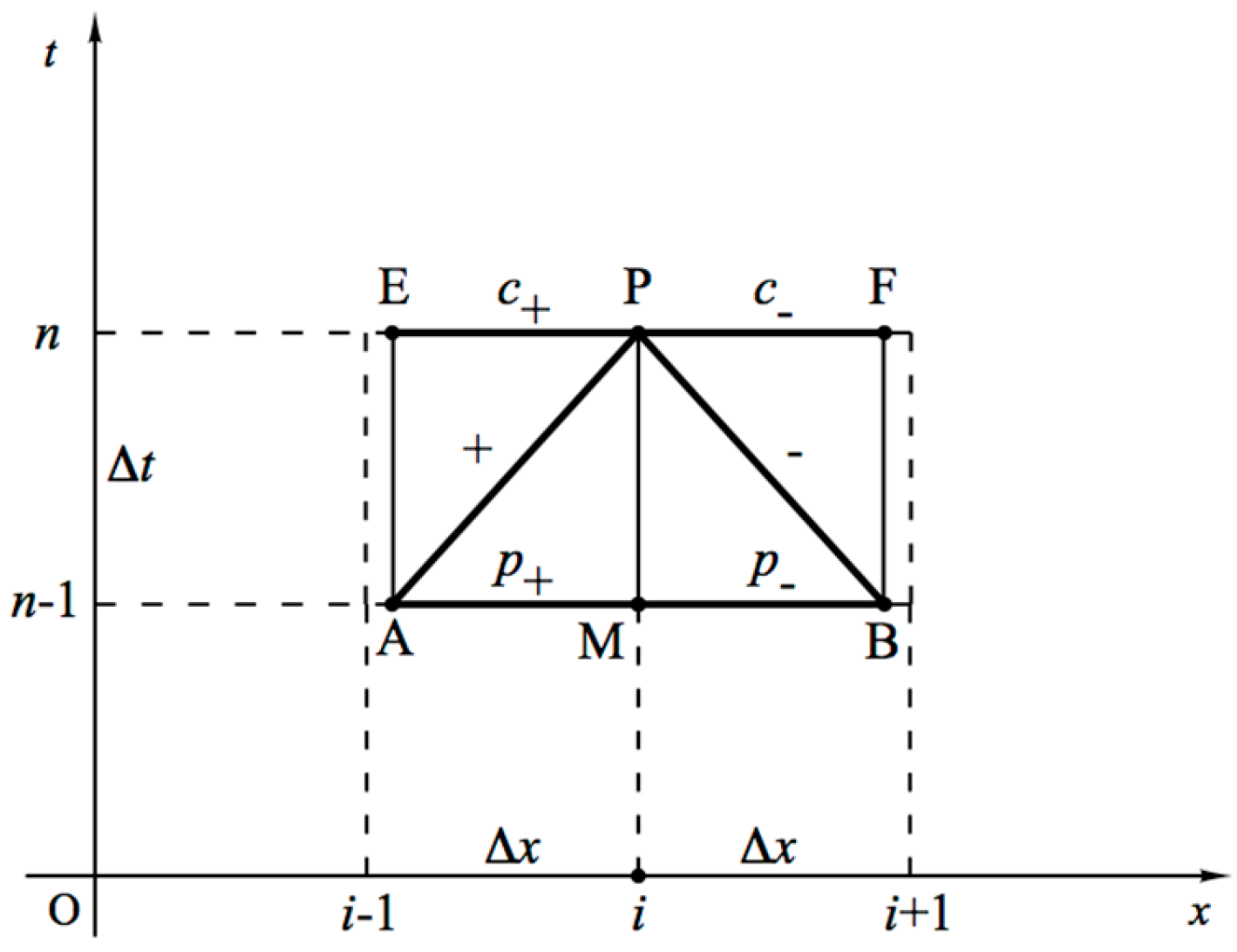
Figure 2.
Comparison between numerical and experimental pressure for Test 6 and GKV3 model: (a) = 1, (b) = 0.99, (c) = 0.95, and (d) = 0.9.
Figure 2.
Comparison between numerical and experimental pressure for Test 6 and GKV3 model: (a) = 1, (b) = 0.99, (c) = 0.95, and (d) = 0.9.

Figure 3.
MAE obtained for the GKV1 model (a) and for the GKV3 (b) model and different Courant numbers.
Figure 3.
MAE obtained for the GKV1 model (a) and for the GKV3 (b) model and different Courant numbers.
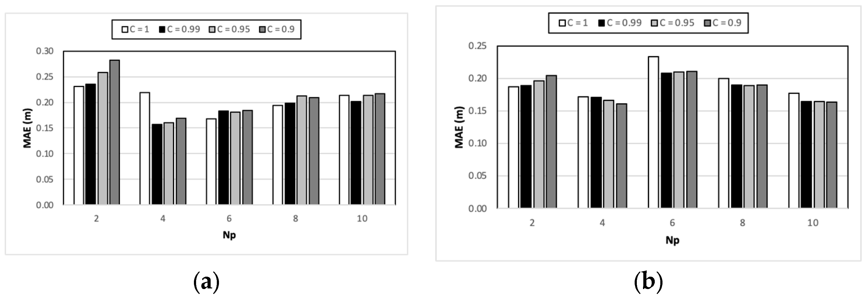
Figure 4.
Comparison between numerical and experimental pressure for Test 8: (a) KV model, (b) GKV1 model, (c) GKV2 model, and (d) GKV3 model.
Figure 4.
Comparison between numerical and experimental pressure for Test 8: (a) KV model, (b) GKV1 model, (c) GKV2 model, and (d) GKV3 model.

Figure 5.
Comparison between numerical and experimental pressure for KV model: (a) Test 2, (b) Test 4, (c) Test 6, and (d) Test 10.
Figure 5.
Comparison between numerical and experimental pressure for KV model: (a) Test 2, (b) Test 4, (c) Test 6, and (d) Test 10.
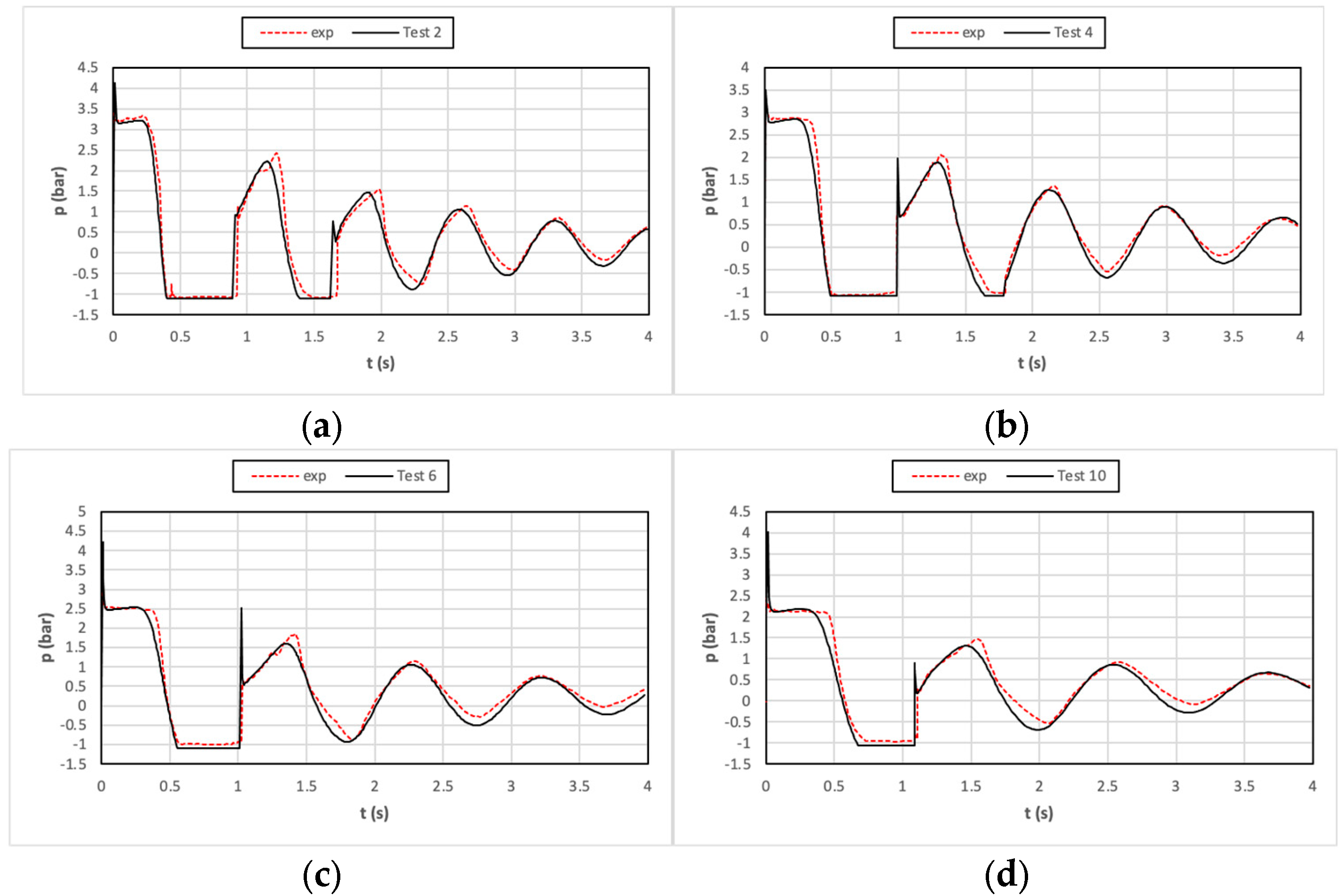
Figure 6.
Comparison between numerical and experimental pressure for GKV2 model: (a) Test 2, (b) Test 4, (c) Test 6, and (d) Test 10.
Figure 6.
Comparison between numerical and experimental pressure for GKV2 model: (a) Test 2, (b) Test 4, (c) Test 6, and (d) Test 10.

Figure 7.
Vapour fraction at the valve computed by the GKV2 model: (a) Test 2, (b) Test 4, (c) Test 6, and (d) Test 10.
Figure 7.
Vapour fraction at the valve computed by the GKV2 model: (a) Test 2, (b) Test 4, (c) Test 6, and (d) Test 10.
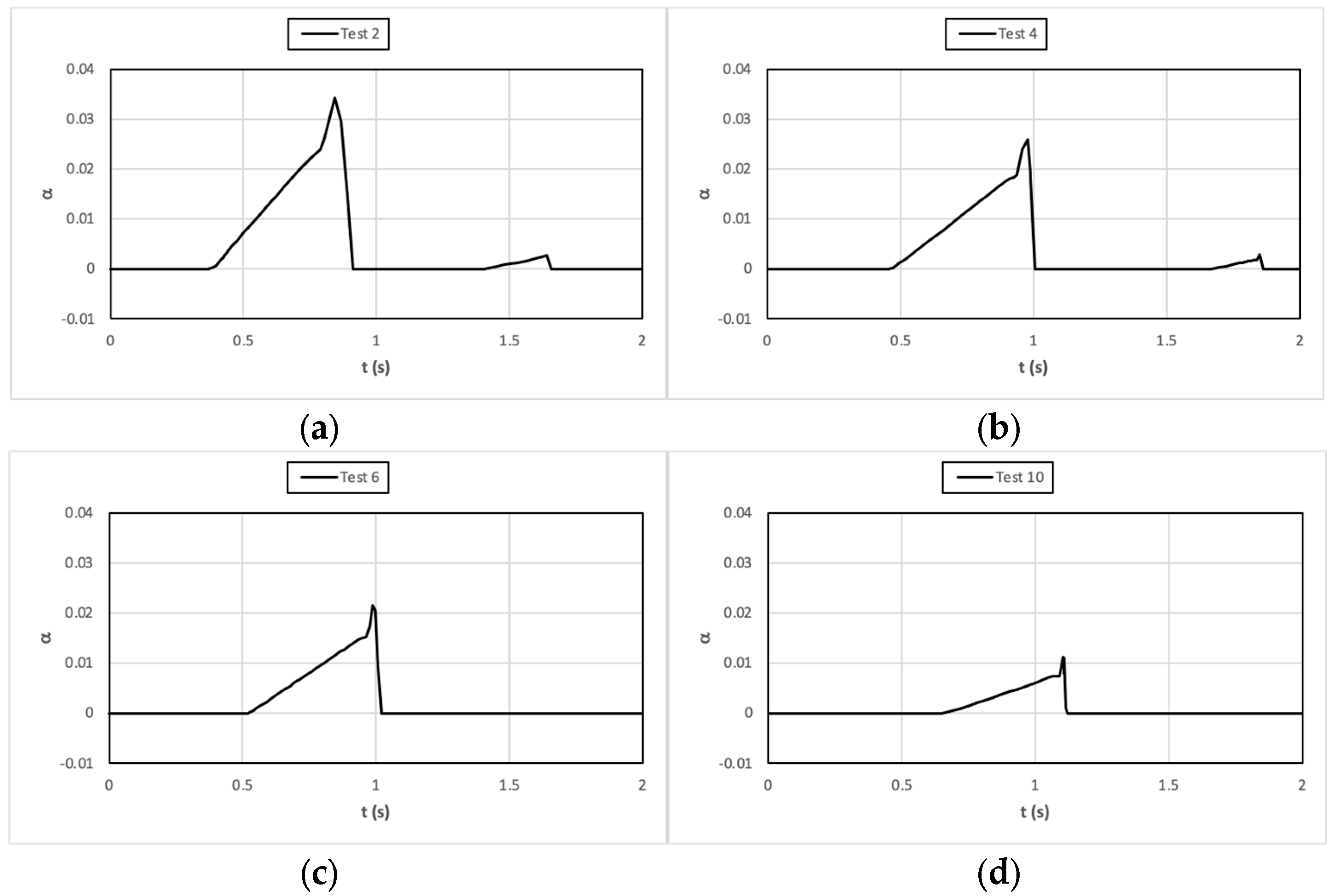
Figure 8.
MAE obtained for the tests without cavitation (a) and for the tests with cavitation (b).


Table 1.
Physical parameters of the Güney [4] experiments with cavitation.
Table 1.
Physical parameters of the Güney [4] experiments with cavitation.
| Test | (°C) | (m/s) | (m) |
|---|---|---|---|
| 2 | 13.8 | 1.28 | 2.88 |
| 4 | 25.0 | 1.37 | 2.99 |
| 6 | 31.0 | 1.34 | 2.98 |
| 8 | 35.0 | 1.37 | 2.98 |
| 10 | 38.5 | 1.33 | 2.93 |
Table 2.
Model parameters [22].
Table 2.
Model parameters [22].
| Test | 2 | 4 | 6 | 8 | 10 | |
| (°C) | 13.8 | 25.0 | 31.0 | 35.0 | 38.5 | |
| KV | (GPa) | 0.6038 | 0.4063 | 0.3321 | 0.2813 | 0.2453 |
| (ms) | 11.20 | 15.63 | 19.16 | 22.66 | 25.92 | |
| GKV1 | (GPa) | 547.8 | 732.6 | 583.8 | 478.8 | 580.1 |
| (GPa) | 0.6050 | 0.4076 | 0.3351 | 0.2915 | 0.2427 | |
| (ms) | 11.00 | 15.35 | 18.64 | 21.36 | 25.71 | |
| GKV2 | (GPa) | 1.221 | 0.6681 | 0.5667 | 0.4099 | 0.3694 |
| (GPa) | 1.265 | 1.436 | 1.071 | 1.698 | 0.9070 | |
| (ms) | 6.243 | 5.943 | 11.38 | 17.11 | 17.52 | |
| (GPa) | 2.010 | 2.038 | 1.476 | 1.314 | 0.9980 | |
| (ms) | 406.5 | 130.0 | 244.9 | 130.0 | 292.1 | |
| GKV3 | 1.652 | 0.8416 | 0.7386 | 0.6641 | 0.5259 | |
| 1.190 | 1.193 | 1.070 | 0.9610 | 0.8950 | ||
| 4.010 | 2.207 | 1.894 | 2.005 | 2.057 | ||
| 2.325 | 2.008 | 1.032 | 0.8490 | 0.6470 | ||
| 338.3 | 141.8 | 279.7 | 473.0 | 788.0 | ||
| 6.443 | 5.362 | 2.439 | 1.392 | 0.9841 | ||
| 10.76 | 15.73 | 19.50 | 25.84 | 30.81 |
Disclaimer/Publisher’s Note: The statements, opinions and data contained in all publications are solely those of the individual author(s) and contributor(s) and not of MDPI and/or the editor(s). MDPI and/or the editor(s) disclaim responsibility for any injury to people or property resulting from any ideas, methods, instructions or products referred to in the content. |
© 2024 by the author. Licensee MDPI, Basel, Switzerland. This article is an open access article distributed under the terms and conditions of the Creative Commons Attribution (CC BY) license (https://creativecommons.org/licenses/by/4.0/).
Share and Cite
MDPI and ACS Style
Pezzinga, G. MOC-Z Model of Transient Cavitating Flow in Viscoelastic Pipe. Water 2024, 16, 1610. https://doi.org/10.3390/w16111610
AMA Style
Pezzinga G. MOC-Z Model of Transient Cavitating Flow in Viscoelastic Pipe. Water. 2024; 16(11):1610. https://doi.org/10.3390/w16111610
Chicago/Turabian StylePezzinga, Giuseppe. 2024. "MOC-Z Model of Transient Cavitating Flow in Viscoelastic Pipe" Water 16, no. 11: 1610. https://doi.org/10.3390/w16111610
Note that from the first issue of 2016, this journal uses article numbers instead of page numbers. See further details here.