Abstract
Groundwater contamination source (GCS) parameter identification can help with controlling groundwater contamination. It is proverbial that groundwater contamination concentration observation errors have a significant impact on identification results, but few studies have adequately quantified the specific impact of the errors in contamination concentration observations on identification results. For this reason, this study developed a Bayesian-based integrated approach, which integrated Markov chain Monte Carlo (MCMC), relative entropy (RE), Multi-Layer Perceptron (MLP), and the surrogate model, to identify the unknown GCS parameters while quantifying the specific impact of the observation errors on identification results. Firstly, different contamination concentration observation error situations were set for subsequent research. Then, the Bayesian inversion approach based on MCMC was used for GCS parameter identification for different error situations. Finally, RE was applied to quantify the differences in the identification results of each GCS parameter under different error situations. Meanwhile, MLP was utilized to build a surrogate model to replace the original groundwater numerical simulation model in the GCS parameter identification processes of these error situations, which was to reduce the computational time and load. The developed approach was applied to two hypothetical numerical case studies involving homogeneous and heterogeneous cases. The results showed that RE could effectively quantify the differences caused by contamination concentration observation errors, and the changing trends of the RE values for GCS parameters were directly related to their sensitivity. The established MLP surrogate model could significantly reduce the computational load and time for GCS parameter identification. Overall, this study highlights that the developed approach represents a promising solution for GCS parameter identification considering observation errors.
1. Introduction
It is essential to obtain information on groundwater contamination sources (GCSs) to assess contamination risks and develop contamination remediation [1,2]. However, due to groundwater contamination occurring underground, it is often difficult to directly obtain GCS parameters (including their number, location, and release history) [3,4]. Therefore, it is necessary to conduct research on GCS parameter identification.
At present, simulation–optimization approaches and Bayesian inversion approaches are the most widely used approaches for GCS parameters identification [5,6,7]. Compared to simulation–optimization approaches, Bayesian inversion approaches can better describe the uncertainty of identification results [8,9]. However, for groundwater systems characterized by high-dimensional nonlinearity, the posterior probability distributions of the unknown parameters inferred by the Bayesian inversion approach usually take the form of multiplication [10]. Therefore, it is necessary to apply sampling statistical approaches to sample from the posterior probability distribution to obtain its statistical characteristics. Markov chain Monte Carlo (MCMC) [11,12] can generate samples from the posterior probability distribution of parameters and conduct statistical analysis efficiently [13,14]. MCMC has been successfully used for GCS parameter identification many times [4,15,16,17,18].
In practice, the obtained contamination concentration observations inevitably contain errors during GCS parameter identification. In fact, many researchers have realized the impact of errors in contamination concentration observations on GCS parameter identification results. For example, Skaggs and Kabala (1994) [19] used the Tikhonov Regularization (TR) approach to identify the release history of GCSs and found that plume observation errors could affect identification results. Woodbury and Ulrych (1996) [20] conducted GCS parameter identification using minimum relative entropy, considering the impact of observed data errors. Chen et al. (2018) [21] identified GCS information using a restart ensemble Kalman filter and found that contamination concentration observation errors had a significant impact on identification results. Furthermore, some studies have also attempted to use some approaches, such as wavelet analysis, to reduce contamination concentration observation errors and improve GCS parameter identification accuracy [22,23]. However, few studies have quantified the specific impact of the errors in contamination concentration observations on identification results. Fortunately, relative entropy (RE) can effectively quantify the differences between different posterior probability distributions that are inferred using the Bayesian inversion approach based on MCMC.
In addition, using the Bayesian inversion approach for parameter identification requires running groundwater numerical simulation models thousands of times, which results in a significant amount of computation time and load [17,18]. Establishing a surrogate model for the original groundwater numerical model is an effective way to solve this problem [15,24,25]. The commonly used approaches for constructing surrogate models include polynomial regression [26], radial basis functions [27,28], artificial neural networks [29,30], support vector machine regression (SVR) [31,32], extreme learning machines [33], Kriging [15,34], etc. Compared to these approaches, Multi-Layer Perceptron (MLP) introduces one or more hidden layers on the basis of a single-layer neural network [35,36], which can be more effectively applied to the regression for high-dimensional nonlinear systems, such as the groundwater system [37]. Hence, MLP can be applied to build a surrogate model for the high-precision replacement based on the input–output datasets of the original groundwater numerical simulation model. After constructing a surrogate model, directly calling the surrogate model in the Bayesian inversion approach for GCS parameter identification can reduce calculation time and load.
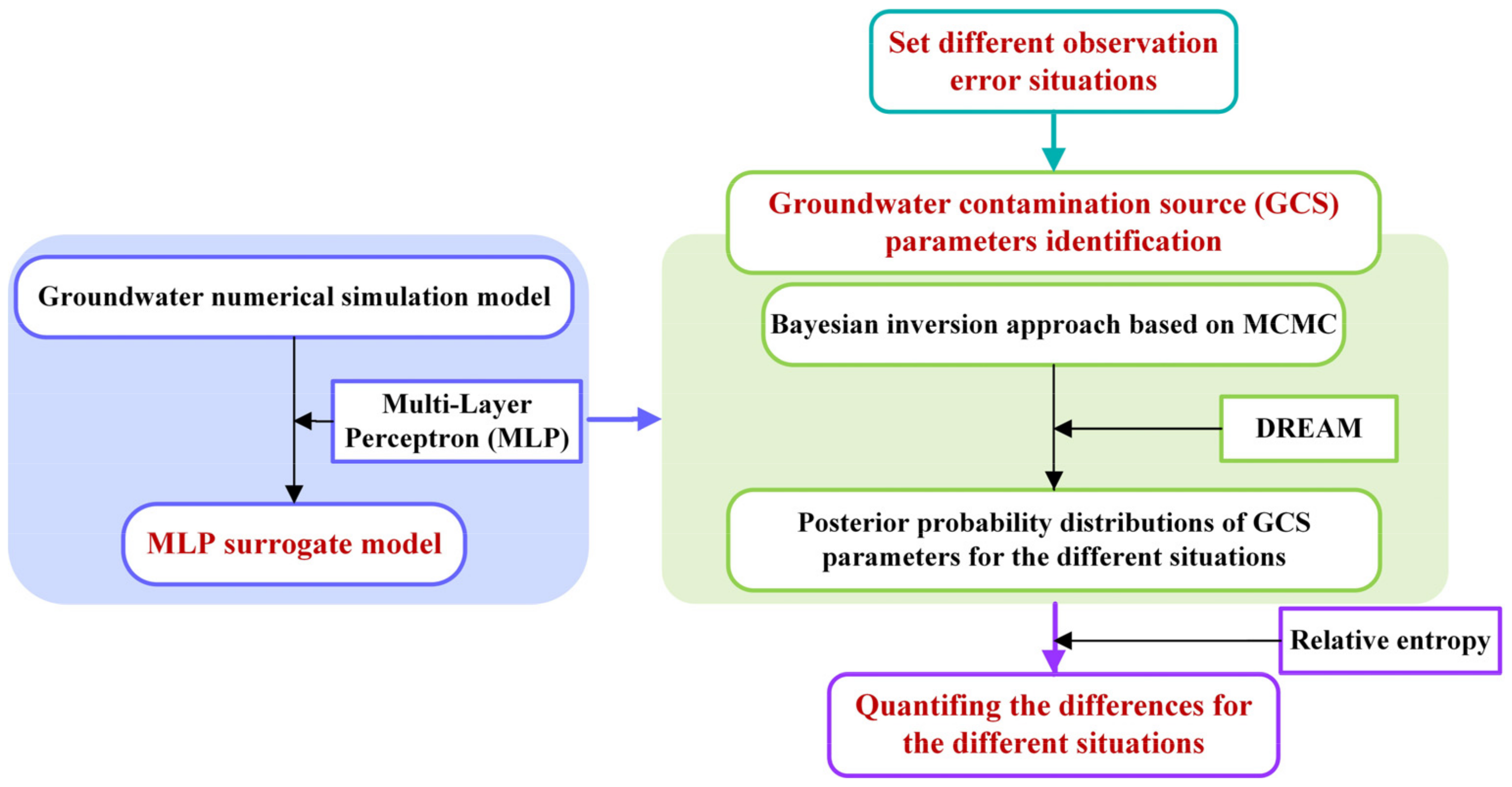
To this end, this study developed a Bayesian-based integrated approach that combined MCMC, RE, MLP, and surrogate modeling for GCS parameter identification and quantifying the impact of groundwater contamination concentration observation errors on it. The Bayesian inversion approach based on MCMC was used to identify unknown GCS parameters. Meanwhile, RE was used to quantify differences caused by groundwater contamination concentration observation errors by setting different error situations. Furthermore, a surrogate model was established using the MLP approach for the original groundwater numerical simulation model to reduce the calculation time and load in GCS parameter identification. The research framework of this study is presented in Figure 1. The remainder of this paper is organized as follows. The methodology of this study is presented in Section 2. Two hypothetical numerical case studies were introduced to develop exploration in Section 3. In Section 4, the results and discussions were presented. Finally, some conclusions were given in Section 5.

Figure 1.
The research framework of this study.
2. Methodology
2.1. Simulation Model
The numerical simulation model for groundwater includes a groundwater flow model and a groundwater solute transport model, the latter of which needs to be constructed based on the former. The partial differential equations of groundwater flow and solute transport are derived based on the law of conservation of mass and Taylor’s formula, among others. The partial differential equation describing the two-dimensional unsteady flow of unconfined groundwater through saturated aquifers can be written as follows:
The two-dimensional groundwater solute transport model may be given as follows:
Equation (2) can be related to Equation (1) using Darcy’s Law:
where and are the distances along the respective Cartesian coordinate axes (); is a principal component of the hydraulic conductivity tensor in the corresponding coordinate direction (); is the hydraulic head (); is the water inflow or outflow from the aquifer per unit of area in the vertical direction per unit time (); is the specific yield; is the time (); is the concentration of contaminants dissolved in groundwater (); is the porosity of the porous medium; is the flow velocity (); is the change in solute mass in unit volume aquifer per unit time (); is the hydrodynamics dispersion tensor (), and is described as follows:
where and are the components of pore water velocity; is its magnitude; and and denote longitudinal and transverse dispersivities, respectively.
In this study, the groundwater flow and solute transport equations were, respectively, solved by the MODFLOW program [38] and the MT3DMS program [39].
2.2. Parameter Identification
In this study, a group of disturbed contamination concentration observations were generated by adding stochastic disturbances based on Gaussian distribution to account for the errors in groundwater contamination concentration observations:
where indicates the raw groundwater contamination concentration observations, which could be obtained by putting the set true values of the unknown GCS parameters into the groundwater numerical simulation model, and is the small tuning parameter that represents the strength of disturbances for observations. According to different values of , we set six error situations, as shown in Table 1.

Table 1.
The six situations for different observation errors.
2.2.1. Bayesian Inversion
In this study, we used the Bayesian inversion approach to identify unknown GCS parameters in different error situations. The Bayesian inversion approach is a probabilistic inversion approach, and its mathematical foundation is the Bayesian formula. Its expression is described [40] as follows:
where represents the unknown GCSs parameters; represents contamination concentration observations; is the prior information of the unknown GCS parameter; is the likelihood; is usually regarded as a normalization constant; and is the posteriori probability distribution, i.e., the unknown GCSs parameter identification results.
It is often difficult to directly obtain the analytical form for for the groundwater numerical simulation model. We used MCMC to draw samples from and conduct statistical analysis in this study.
2.2.2. Markov Chain Monte Carlo
The Markov chain Monte Carlo (MCMC) can construct a suitable Markov chain during the sampling process, which can reach a stationary distribution, i.e., the posterior probability distribution . Then, the samples are extracted from using a sampling approach [41]. Additionally, the samples are used for obtaining the statistical characteristics of . In this study, we utilized the Differential Evolution Adaptive Metropolis (DREAM), which is the multi-chain MCMC sampling algorithm, to generate samples and conduct statistics. Detailed information on the DREAM approach is described in Vrugt et al. (2009) [42].
To ensure the stable convergence of the Markov chain during the GCS parameter identification process, the Gelman–Rubin approach [43] was used for convergence diagnosis, and the convergence diagnosis indicators could be expressed as follows:
where is the diagnostic index; denotes the Markov chain length; denotes the number of Markov chains; denotes the variance of the average value for Markov chains; ρ denotes the average value of the intra-chain variance of Markov chains. Usually, when the value is less than 1.2, it can be considered that the Markov chain reaches a stable convergence state; that is, the sampling process of the algorithm converges.
2.3. Relative Entropy
Relative entropy (RE), also known as Kullback–Leibler divergence or information divergence, can be used to measure the difference between two probability distributions effectively [9]. RE is an important concept in information theory. In this study, the larger the relative entropy, the greater the difference in the posterior probability distribution of GCS parameters due to observation errors, which means that the information between them is more different.
To quantify the impact of contamination concentration observation errors on the posterior probability distributions of unknown GCS parameters, we used RE to quantify the differences between the posterior probability distributions obtained under the six simulations (as shown in Table 1), wherein S1 was the control situation. The calculation equation of RE is as follows [44]:
where is the value of RE between the posterior probability distribution of unknown GCS parameters in S1 and the posterior probability distributions of unknown GCS parameters in the situation; denotes the posterior probability distributions of unknown GCS parameters for S1; denotes the posterior probability distributions of unknown GCS parameters for the situation, .
2.4. Multi-Layer Perceptron
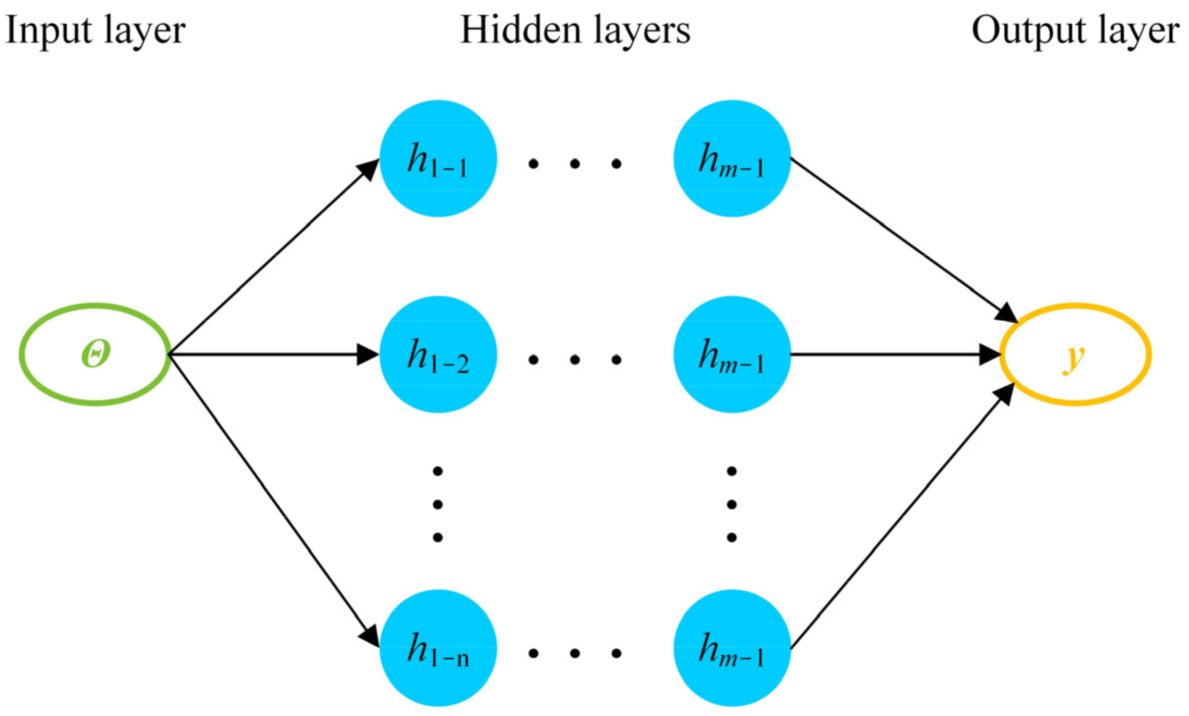
Multi-Layer Perceptron (MLP) is a deep learning approach based on feedforward neural networks [36]. It is essentially a supervised learning algorithm that can learn a function by training on a dataset. MLP can learn a nonlinear function approximator for regression by giving a set of features and a target , where is the number of input dimensions. Different from logistic regression, MLP has one or more nonlinear hidden layers between the input and output layers, as shown in Figure 2.
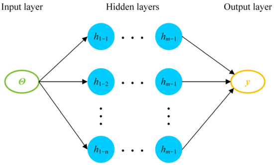
Figure 2.
MLP approach structure diagram [37].
The regression function of MLP can be expressed as follows [45]:
where is the input; is the output; ω denotes the weight; denotes the bias; is the hidden layers number; and is the activation function, which usually chooses nonlinear functions such as Sigmoid, Tanh, and ReLU. Their expressions are given as follows:
In this study, ReLU was adopted as the activation function. The MLP surrogate model structure included four hidden layers, each with 10 neurons. Additionally, the solving algorithm used was ‘lbfgs’, while the maximum number of iterations was set to 1000.
3. Numerical Applications
This study applied the above methodology to two hypothetical case studies, including a homogeneous case and a heterogeneous case. One of the advantages of using the hypothetical case study is that the calculated results can be compared with the theoretical results directly, so the research results can be clearly and accurately presented [46]. Moreover, the calculation programs were all written in Python 3.12.1 in this study.
3.1. Case Studies
3.1.1. Case 1
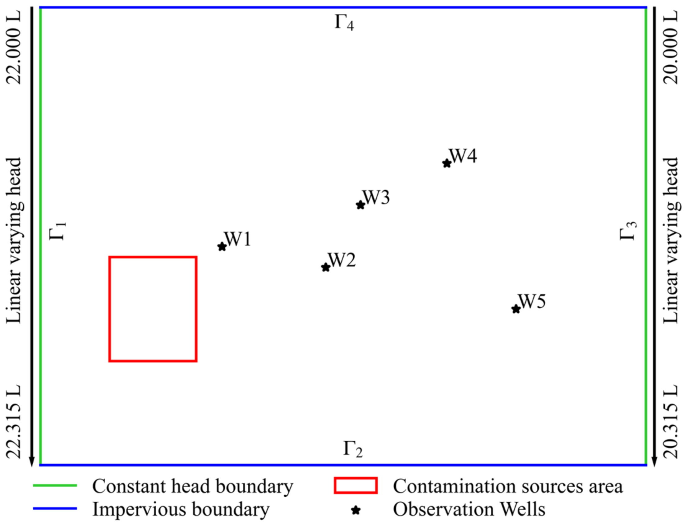
The groundwater flow field range of Case 1 was . This was a two-dimensional groundwater flow field, with both upper and lower boundaries being impermeable and both left and right boundaries being linearly varying water heads, as shown in Figure 3. In the flow field, there were a total of five observation wells, and all of them obtained groundwater contamination concentration observations at . In this case study, it was assumed that the location ( and ), intensity (), and initial release time () of the GCSs were unknown to be required identification, and they all followed the uniform distribution. Additionally, their prior ranges and set true values are presented in Table 2. Meanwhile, other parameters, such as the hydraulic conductivity (), end release time (), porosity (), and dispersivities ( and ), were considered known, which are given in Table 3. Furthermore, we assumed that there was only one contamination source.
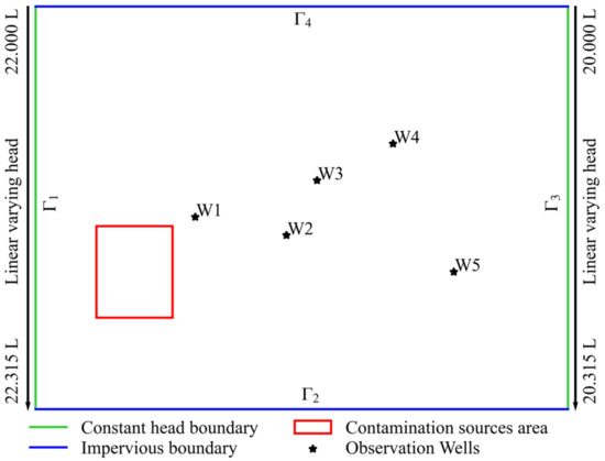
Figure 3.
Groundwater flow field diagram of Case 1 showing the boundary conditions, contamination source areas, and observation wells.
Table 2.
The prior ranges and true values of unknown GCS parameters for Case 1.
Table 3.
Parameter values of simulation model for Case 1.
3.1.2. Case 2
The boundary of the flow field in Case 2 was irregular, as shown in Figure 4. The unknown GCS parameters of Case 2 were still the location ( and ), intensity (), and initial release time (), but their true values and prior distribution ranges were different from Case 1, as shown in Table 4. The end release time (), porosity (), number of contaminants, and the dispersivities’ ( and ) and time to obtain groundwater contamination concentration observations were the same as in Case 1, while the conductivity field was divided into three hydraulic conductivity zones with a hydraulic conductivity of 15, 12, and 10 ().
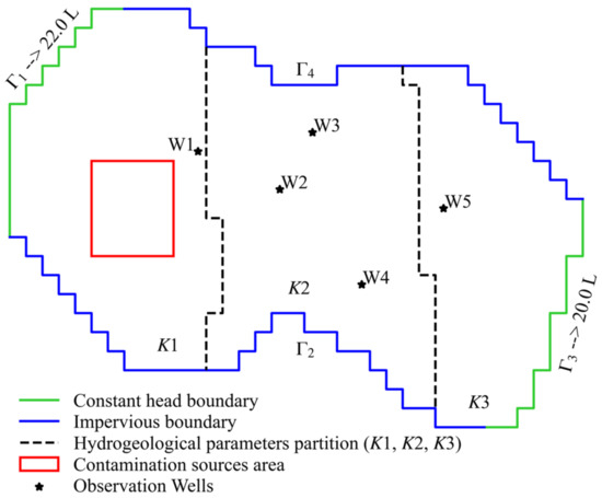
Figure 4.
Groundwater flow field diagram of Case 2 showing the boundary conditions, contamination source area, and observation wells.
Table 4.
The prior ranges and true values of unknown GCS parameters for Case 2.
3.2. Surrogate Modeling
To reduce the computational time and load of GCS parameter identification, a surrogate model was established for the original groundwater numerical simulation model using the MLP approach. Meanwhile, to present the superiority of the MLP approach in surrogate modeling, support vector machine regression (SVR) and Kriging were also used to establish surrogate models, and their approximation accuracy to the original groundwater numerical simulation model was compared with the MLP surrogate model.
Firstly, 500 sets of training samples and 200 sets of test samples were extracted from the prior distribution of unknown GCS parameters presented in Section 3.1. Next, the training and test samples were put into the original groundwater numerical simulation model to obtain 500 sets of output results and 200 sets of output results, respectively; thus, we obtained 500 sets of input–output datasets and 200 sets of input–output datasets. Then, the MLP surrogate model, Kriging surrogate model, and SVR surrogate model were established for the original groundwater numerical simulation model based on 500 sets of input–output datasets. Finally, the relative error was used to evaluate the accuracy of the three surrogate models to conduct a comparative analysis. More specifically, 200 sets of test samples were separately put into MLP surrogate models, the Kriging surrogate model, and the SVR surrogate model to obtain the corresponding model outputs and compare these outputs with the outputs of the original groundwater numerical simulation model. The expression of relative error can be given as follows:
3.3. Computation Time Analysis
To improve the efficiency of GCS parameter identification was one of the main objectives of this study. Therefore, we compared the execution time of the original groundwater numerical simulation model with that of the MLP surrogate model to evaluate whether efficiency was improved. In addition, the advantages of the MLP surrogate model could be verified in both homogeneous and heterogeneous situations by simultaneously setting Cases 1 and 2.
4. Results and Discussions
4.1. Analysis of the Surrogate Model
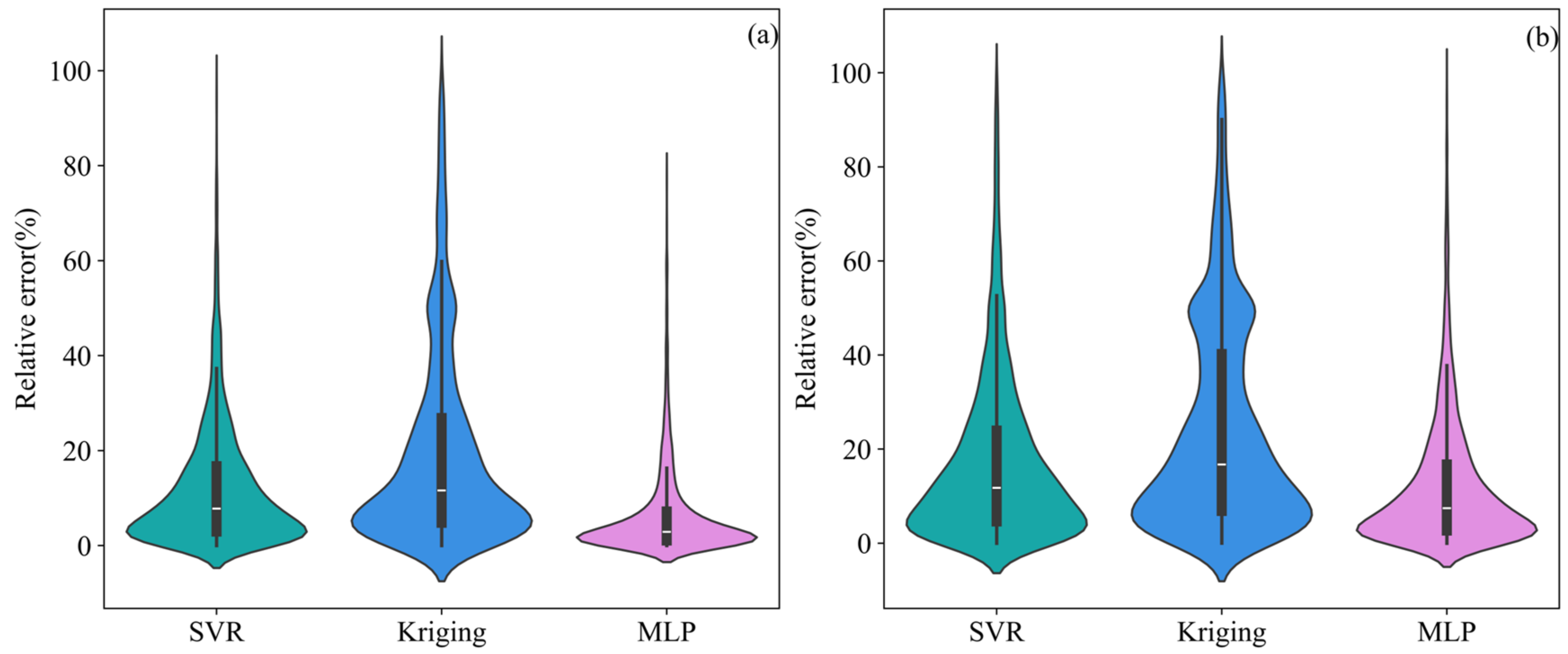
To demonstrate the advantages of the MLP surrogate model, we compared its accuracy with that of the Kriging surrogate model and SVR surrogate model, as shown in Figure 5. These were the relative errors between the groundwater contamination concentration outputs of the original groundwater numerical simulation model and that of the surrogate models. Additionally, these outputs were obtained for 200 sets of test samples at the time step . Figure 5 shows that the relative error values between the concentration outputs of the MLP surrogate model and those of the original groundwater numerical simulation model were very small in both case studies, indicating that the MLP surrogate model could accurately approximate the original groundwater numerical simulation model. Clearly, the accuracy of the MLP surrogate model was superior to that of the Kriging surrogate model and the SVR surrogate model for both Case 1 and Case 2. This indicates that the MLP surrogate model could maintain its superiority in both homogeneous and heterogeneous media, which is to say, MLP was the best approach for establishing the surrogate model among these three approaches. This is mainly because MLP is a deep learning approach that includes hidden layers, which are more suitable for high-dimensional systems, such as groundwater models. Therefore, the MLP surrogate model could be directly used for GCS parameter identification, which not only improved overall computational efficiency but also maintained high accuracy. Moreover, the accuracy of the surrogate models in Case 1 was better than that in Case 2, which may be because Case 2 was heterogeneous and irregular.
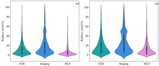
Figure 5.
Accuracy of SVR surrogate model, Kriging surrogate model, and MLP surrogate model for Case 1 (a) and Case 2 (b).
4.2. Analysis of the Parameter Identification Results
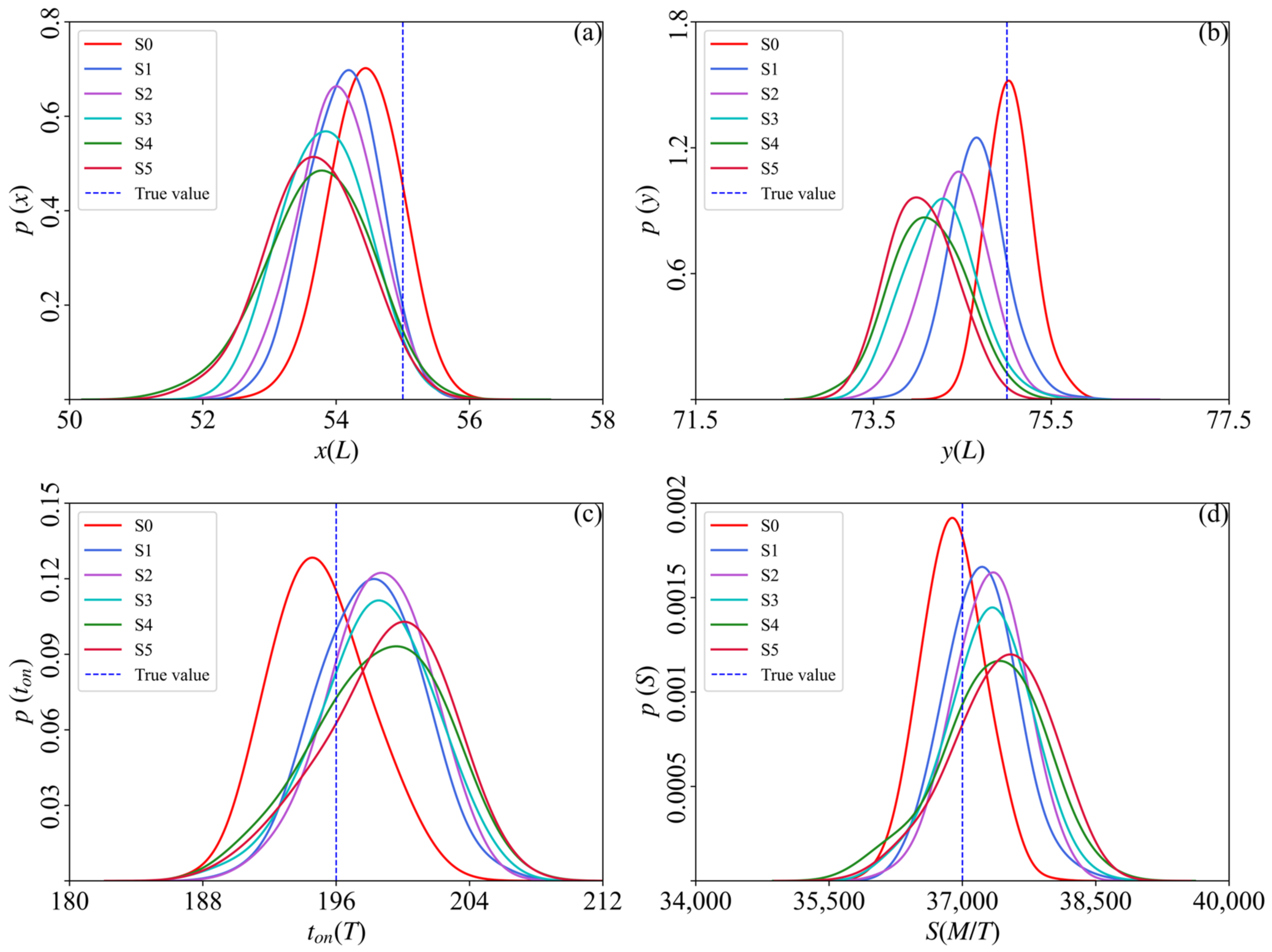
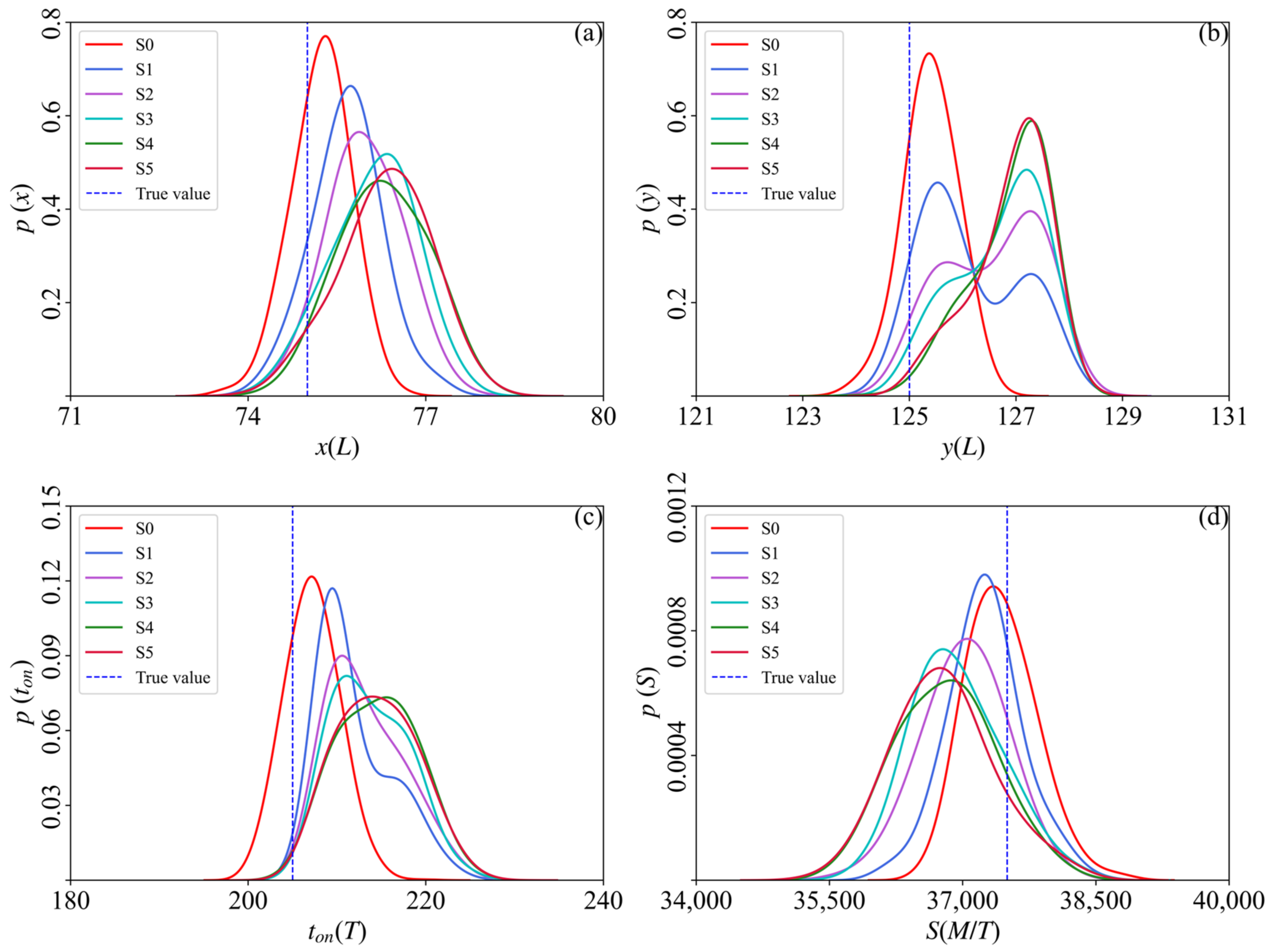
The DREAM algorithm was set with an acceptance rate of 0.7, iterations of 50,000, and a crossover rate of 0.3. In the stable convergence stage, we would use the last 20,000 sets of samples to estimate the statistical characteristics of the posterior probability distribution for the unknown GCS parameters in this study. The posterior probability distributions obtained under different concentration observation error sizes are shown in Figure 6 and Figure 7. It could be seen that as the concentration observation errors increased, overall, the maximum a posteriori probability (MAP) was further away from the set parameter true values. This indicates that the concentration of observation errors had a significant impact on the identification results. However, there were also abnormal situations; for example, in Case 1, the identification accuracy of in S4 was lower than that in S5. This should be related to the randomness of the Bayesian inversion approach itself and also influenced by the differences between the original numerical simulation model and the MLP surrogate model. Moreover, observation errors had varying degrees of impact on the identification results of different GCS parameters. For example, observation errors had a more significant impact on the identification results of than that on the identification results of other GCS parameters. This may be related to the sensitivity of the GCS parameters.
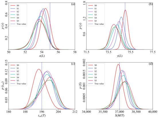
Figure 6.
Posterior probability distributions for , (a), (b), (c), and (d) under different observation error situations in Case 1.
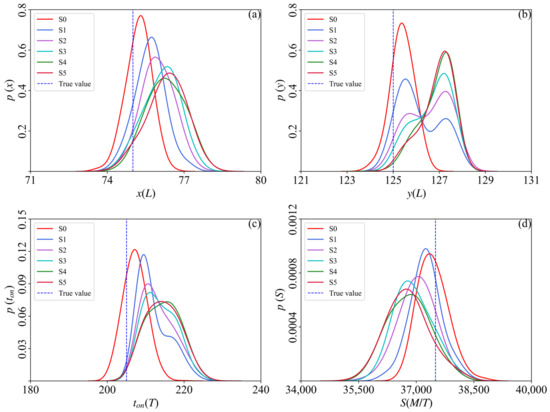
Figure 7.
Posterior probability distributions for , (a), (b), (c), and (d) under different observation error situations in Case 2.
Furthermore, the established MLP surrogate model could reduce the computational time in the GCS parameter identification process effectively. The CPU time required for the original groundwater numerical simulation model to complete 1000 simulations is about 32 min, while the MLP surrogate model can complete 50,000 simulations in only about 195 min (on a PC with AMD R5-3600X 3.80 GHz processor and 16 GB RAM, Xi’an, China). The established MLP surrogate model has a short computation time and high approximation accuracy for the complex simulation model, which promotes its application in solving GCS parameter identification problems.
4.3. Analysis of the Relative Entropy
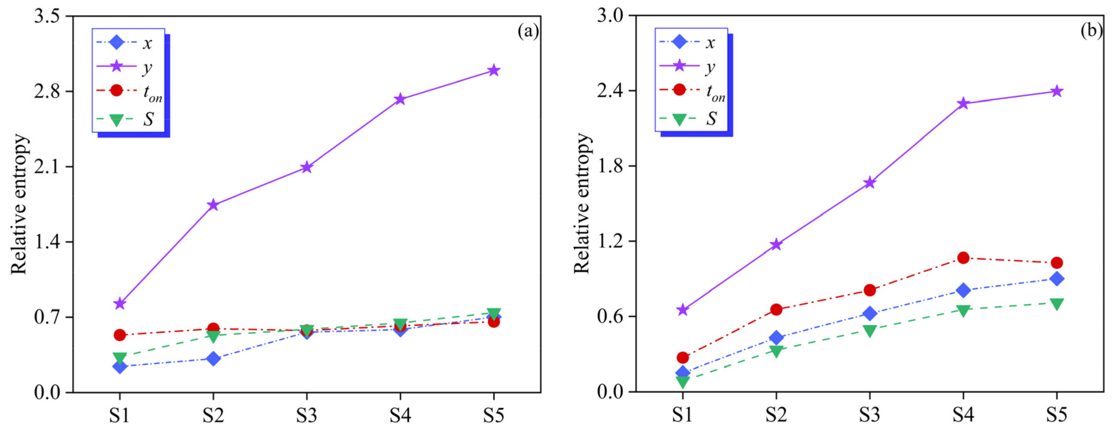
RE was used to quantify the differences caused by errors in groundwater contamination concentration observations in this study. The RE values calculated based on Equation (8) are shown in Figure 8. Figure 8a,b, respectively, present the RE values of Case 1 and Case 2. As can be seen from Figure 8, even when the errors in groundwater contamination concentration observations were small, a clear RE value could still be calculated; that is, small errors could still have a significant impact on posterior probability distributions (i.e., the GCS parameter identification results). As the error increased, the impact on the identification results became more pronounced, which indicated that the influence of groundwater contamination concentration observation errors cannot be ignored in GCS parameter identification. Meanwhile, the degree of influence gradually slowed down as the error increased. It may be related to the calculation approach of RE. However, there were abnormal situations in this pattern, such as in Case 2, where the RE value of in S4 was slightly lower than in S5. This was because the error between the constructed MLP surrogate model and the original model may have had an impact on the GCS parameter identification results. It should be noted that although the constructed surrogate model often has high accuracy and can approximate the original groundwater numerical simulation model well, surrogate models belong to the black box model and have limitations. Generally, surrogate models are often used for processes that require multiple calls to the complex simulation model, such as the iterative solving of optimization models and uncertainty analysis.
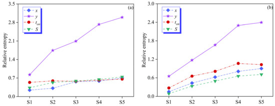
Figure 8.
Relative entropy values of different observation error situations for Case 1 (a) and Case 2 (b).
Furthermore, the RE values of were greater than those of other parameters and had a more pronounced trend of change. This may be related to the sensitivity of the parameters. To verify this issue, we used the LH-OAT (Latin-Hypercube One-factor-At-a-time) approach [47] to conduct a sensitivity analysis on the GCS parameters. It combines the uniformity of LH sampling with the accuracy of the OAT algorithm, ensuring the reliability and stability of each parameter’s analysis result. LH-OAT first divides the parameter space with parameters into layers based on the principle of LH sampling. Then, it randomly samples from each layer for each parameter to generate a sampling parameter group. Then, based on the OAT approach, only minor perturbations are applied to one parameter at a time while keeping the other parameters unchanged, and the model needs to be run times to analyze the sensitivity of the parameter. The above disturbance analysis process is repeated to complete the analysis for all parameters, so a total of runs are required. The calculation equation of LH-OAT is as follows:
where is the model operator; is the sampling value of the ith parameter in the layer; is the degree of disturbance of parameter ; and is the relative sensitivity of parameter in the kth layer.
The global sensitivity of parameters can be calculated by :
In this study, the LH sampling frequency was set to 1000 while the OAT algorithm disturbance was set to 5%. Additionally, the sensitivity calculation was based on the MLP surrogate model. The sensitivity calculation results are shown in Figure 9. As shown in Figure 9, the sensitivity of was greater than that of other parameters. Therefore, the trend of the RE value of change in the GCS parameter was directly related to its sensitivity.
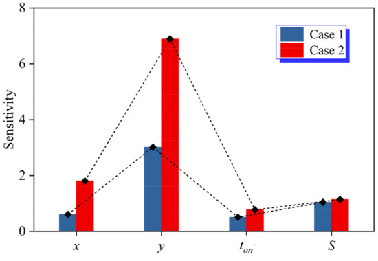
Figure 9.
Sensitivity of the GCS parameters for the two cases.
5. Conclusions
This study developed a Bayesian-based integrated approach that combined Markov chain Monte Carlo (MCMC), relative entropy (RE), Multi-Layer Perceptron (MLP), and surrogate modeling to identify unknown groundwater contamination source (GCS) parameters and quantify the impact of groundwater contamination concentration observation errors. The Bayesian inversion approach based on MCMC was applied to identify unknown GCS parameters and generate their posterior probability distributions. Then, RE was used to quantify the posterior probability distribution differences caused by groundwater contamination concentration observation errors. Meanwhile, a surrogate model for the original groundwater numerical simulation model was established using the MLP approach to improve the calculation time and load in GCS parameter identification. Through case studies of homogeneous and heterogeneous media, the following findings can be summarized: RE can effectively quantify the differences between posterior probability distributions, and the changing trends of the RE values for GCS parameters were directly related to their sensitivity. The MLP surrogate model could reduce the computational load and time for GCS parameters identification significantly, which represented an improvement in the efficiency of the identification process. However, the research conclusion may be affected by fitting errors between surrogate models and simulation models. The specific impact of fitting errors on GCS parameter identification results will be further investigated in future research. In addition, this study found that the sensitivity of GCS parameters had a significant impact on its identification results. How to further improve identification accuracy based on this discovery will also be the focus of our future research.
Author Contributions
Methodology, X.Y.; Formal analysis, Y.A.; Writing—original draft, X.Y.; Supervision, Y.A. All authors have read and agreed to the published version of the manuscript.
Funding
This study was supported by the Natural Science Basic Research Program of Shanxi (2023-JC-QN-0290).
Data Availability Statement
Data are contained within the article.
Conflicts of Interest
The authors declare no conflicts of interest.
References
- Jha, M.K.; Datta, B. Linked simulation-optimization based dedicated monitoring network design for unknown pollutant source identification using dynamic time warping distance. Water Resour. Manag. 2014, 28, 4161–4182. [Google Scholar] [CrossRef]
- Kontos, Y.N.; Kassandros, T.; Perifanos, K.; Karampasis, M.; Katsifarakis, K.L.; Karatzas, K. Machine learning for groundwater pollution source identification and monitoring network optimization. Neural Comput. Appl. 2022, 34, 19515–19545. [Google Scholar] [CrossRef] [PubMed]
- Ayvaz, M.T. A hybrid simulation–optimization approach for solving the areal groundwater pollution source identification problems. J. Hydrol. 2016, 538, 161–176. [Google Scholar] [CrossRef]
- Yan, X.; Dong, W.; An, Y.; Lu, W. A Bayesian-based integrated approach for identifying groundwater contamination sources. J. Hydrol. 2019, 579, 124160. [Google Scholar] [CrossRef]
- Atmadja, J.; Bagtzoglou, A.C. State of the art report on mathematical methods for groundwater pollution source identification. Environ. Forensics 2001, 2, 205–214. [Google Scholar] [CrossRef]
- Carrera, J.; Alcolea, A.; Medina, A.; Hidalgo, J.; Slooten, L.J. Inverse problem in hydrogeology. Hydrogeol. J. 2005, 13, 206–222. [Google Scholar] [CrossRef]
- Gómez-Hernández, J.J.; Xu, T. Contaminant source identification in aquifers: A critical view. Math. Geosci. 2022, 54, 437–458. [Google Scholar] [CrossRef]
- Ma, X.; Zabaras, N. An efficient Bayesian inference approach to inverse problems based on an adaptive sparse grid collocation method. Inverse Probl. 2009, 25, 035013. [Google Scholar] [CrossRef]
- Zhang, J.; Zeng, L.; Chen, C.; Chen, D.; Wu, L. Efficient Bayesian experimental design for contaminant source identification. Water Resour. Res. 2015, 51, 576–598. [Google Scholar] [CrossRef]
- Gregory, P.C. Bayesian exoplanet tests of a new method for MCMC sampling in highly correlated model parameter spaces. Mon. Not. R. Astron. Soc. 2011, 410, 94–110. [Google Scholar] [CrossRef]
- Hastings, W.K. Monte Carlo sampling methods using Markov chains and their applications. Biometrika 1970, 57, 97–109. [Google Scholar] [CrossRef]
- Metropolis, N.; Rosenbluth, A.W.; Rosenbluth, M.N.; Teller, A.H.; Teller, E. Equation of state calculations by fast computing machines. J. Chem. Phys. 1953, 21, 1087–1092. [Google Scholar] [CrossRef]
- Gamerman, D.; Lopes, H.F. Markov Chain Monte Carlo: Stochastic Simulation for Bayesian Inference, 2nd ed.; Chapman and Hall/CRC: New York, NY, USA, 2006. [Google Scholar]
- Yan, X.; Lu, W.; An, Y.; Dong, W. Assessment of parameter uncertainty for non-point source pollution mechanism modeling: A Bayesian-based approach. Environ. Pollut. 2020, 263, 114570. [Google Scholar]
- An, Y.; Yan, X.; Lu, W.; Qian, H.; Zaiyong, Z. An improved Bayesian approach linked to a surrogate model for identifying groundwater pollution sources. Hydrogeol. J. 2022, 30, 601–616. [Google Scholar] [CrossRef]
- Michalak, A.M.; Kitanidis, P.K. A method for enforcing parameter nonnegativity in Bayesian inverse problems with an application to contaminant source identification. Water Resour. Res. 2003, 39, 1–14. [Google Scholar] [CrossRef]
- Zeng, L.; Shi, L.; Zhang, D.; Wu, L. A sparse grid based Bayesian method for contaminant source identification. Adv. Water Resour. 2012, 37, 1–9. [Google Scholar] [CrossRef]
- Zhang, J.; Zheng, Q.; Chen, D.; Wu, L.; Zeng, L. Surrogate-based Bayesian inverse modeling of the hydrological system: An adaptive approach considering surrogate approximation error. Water Resour. Res. 2020, 56, e2019WR025721. [Google Scholar] [CrossRef]
- Skaggs, T.H.; Kabala, Z.J. Recovering the release history of a groundwater contaminant. Water Resour. Res. 1994, 30, 71–79. [Google Scholar] [CrossRef]
- Woodbury, A.D.; Ulrych, T.J. Minimum relative entropy inversion: Theory and application to recovering the release history of a groundwater contaminant. Water Resour. Res. 1996, 32, 2671–2681. [Google Scholar] [CrossRef]
- Chen, Z.; Gomez-Hernandez, J.J.; Xu, T.; Zanini, A. Joint identification of contaminant source and aquifer geometry in a sandbox experiment with the restart ensemble Kalman filter. J. Hydrol. 2018, 564, 1074–1084. [Google Scholar] [CrossRef]
- Li, J.; Wu, Z.; He, H.; Lu, W. Application of the complementary ensemble empirical mode decomposition for the identification of simulation model parameters and groundwater contaminant sources. J. Hydrol. 2022, 612, 128244. [Google Scholar] [CrossRef]
- Wang, H.; Lu, W.; Chang, Z. Simultaneous identification of groundwater contamination source and aquifer parameters with a new weighted–average wavelet variable–threshold denoising method. Environ. Sci. Pollut. Res. 2021, 28, 38292–38307. [Google Scholar] [CrossRef] [PubMed]
- Mo, S.; Zabaras, N.; Shi, X.; Wu, J. Deep autoregressive neural networks for high-dimensional inverse problems in groundwater contaminant source identification. Water Resour. Res. 2019, 55, 3856–3881. [Google Scholar] [CrossRef]
- Xing, Z.; Qu, R.; Zhao, Y.; Fu, Q.; Ji, Y.; Lu, W. Identifying the release history of a groundwater contaminant source based on an ensemble surrogate model. J. Hydrol. 2019, 572, 501–516. [Google Scholar] [CrossRef]
- He, L.; Huang, G.H.; Zeng, G.M.; Lu, H.W. An integrated simulation, inference, and optimization method for identifying groundwater remediation strategies at petroleum-contaminated aquifers in western Canada. Water Res. 2008, 42, 2629–2639. [Google Scholar] [CrossRef] [PubMed]
- Mugunthan, P.; Shoemaker, C.A.; Regis, R.G. Comparison of function approximation, heuristic, and derivative-based methods for automatic calibration of computationally expensive groundwater bioremediation models. Water Resour. Res. 2005, 41, W11427. [Google Scholar] [CrossRef]
- Regis, R.G.; Shoemaker, C.A. A stochastic radial basis function method for the global optimization of expensive functions. INFORMS J. Comput. 2007, 19, 497–509. [Google Scholar] [CrossRef]
- Mirghani, B.Y.; Zechman, E.M.; Ranjithan, R.S.; Mahinthakumar, G. Enhanced simulation-optimization approach using surrogate modeling for solving inverse problems. Environ. Forensics 2012, 13, 348–363. [Google Scholar] [CrossRef]
- Srivastava, D.; Singh, R.M. Groundwater system modeling for simultaneous identification of pollution sources and parameters with uncertainty characterization. Water Resour. Manag. 2015, 29, 4607–4627. [Google Scholar] [CrossRef]
- Hou, Z.; Lu, W.; Chu, H.; Luo, J. Selecting parameter-optimized surrogate models in DNAPL-contaminated aquifer remediation strategies. Environ. Eng. Sci. 2015, 32, 1016–1026. [Google Scholar] [CrossRef]
- Ouyang, Q.; Lu, W.; Hou, Z.; Zhang, Y.; Li, S.; Luo, J. Chance-constrained multi-objective optimization of groundwater remediation design at DNAPLs-contaminated sites using a multi-algorithm genetically adaptive method. J. Contam. Hydrol. 2017, 200, 15–23. [Google Scholar] [CrossRef] [PubMed]
- Jiang, X.; Lu, W.; Hou, Z.; Zhao, H.; Na, J. Ensemble of surrogates-based optimization for identifying an optimal surfactant-enhanced aquifer remediation strategy at heterogeneous DNAPL-contaminated sites. Comput. Geosci. 2015, 84, 37–45. [Google Scholar] [CrossRef]
- Hemker, T.; Fowler, K.R.; Farthing, M.W.; von Stryk, O. A mixed-integer simulation-based optimization approach with surrogate functions in water resources management. Optim. Eng. 2008, 9, 341–360. [Google Scholar] [CrossRef]
- Basheer, I.A.; Hajmeer, M. Artificial neural networks: Fundamentals, computing, design, and application. J. Microbiol. Methods 2000, 43, 3–31. [Google Scholar] [CrossRef] [PubMed]
- Gardner, M.W.; Dorling, S.R. Artificial neural networks (the multilayer perceptron)—A review of applications in the atmospheric sciences. Atmos. Environ. 1998, 32, 2627–2636. [Google Scholar] [CrossRef]
- An, Y.; Zhang, Y.; Yan, X. An integrated Bayesian and machine learning approach application to identification of groundwater contamination source parameters. Water 2022, 14, 2447. [Google Scholar] [CrossRef]
- McDonald, M.G.; Harbaugh, W. A Modular Three-Dimensional Finite Difference Groundwater Flow Model. In Geological Survey Techniques of Water Resources Investigations Reports; USGS: Reston, VA, USA, 1988; p. 586. [Google Scholar]
- Zheng, C.; Wang, P.P. MT3DMS: A Modular Three-Dimensional Multispecies Transport Model for Simulation of Advection, Dispersion, and Chemical Reactions of Contaminants in Groundwater Systems; Documentation and User’s Guide; U.S. Army Engineer Research and Development Center Contract Report SERDP-99-1; U.S. Army Engineer Research and Development Center: Vicksburg, MS, USA, 1999. [Google Scholar]
- Bayes, T. LII. An essay towards solving a problem in the doctrine of chances. By the late Rev. Mr. Bayes, F.R.S. communicated by Mr. Price, in a letter to John Canton, A. M. F. R. S. Philos. Trans. R. Soc. Lond. 1763, 53, 370–418. [Google Scholar]
- Marshall, L.; Nott, D.; Sharma, A. A comparative study of Markov chain Monte Carlo methods for conceptual rainfall-runoff modeling. Water Resour. Res. 2004, 40, W02501. [Google Scholar] [CrossRef]
- Vrugt, J.A.; ter Braak, C.J.; Diks, C.G.; Robinson, B.A.; Hyman, J.M.; Higdon, D. Accelerating Markov chain Monte Carlo simulation by differential evolution with self-adaptive randomized subspace sampling. Int. J. Nonlinear Sci. Numer. Simul. 2009, 10, 273–290. [Google Scholar] [CrossRef]
- Gelman, A.; Rubin, D.B. Inference from iterative simulation using multiple sequences. Stat. Sci. 1992, 7, 457–472. [Google Scholar] [CrossRef]
- Lindley, D.V. On a measure of the information provided by an experiment. Ann. Math. Stat. 1956, 27, 986–1005. [Google Scholar] [CrossRef]
- Agirre-Basurko, E.; Ibarra-Berastegi, G.; Madariaga, I. Regression and multilayer perceptron-based models to forecast hourly O3 and NO2 levels in the Bilbao area. Environ. Model. Softw. 2006, 21, 430–446. [Google Scholar] [CrossRef]
- Zhao, Y.; Lu, W.; Xiao, C. A Kriging surrogate model coupled in simulation–optimization approach for identifying release history of groundwater sources. J. Contam. Hydrol. 2016, 185, 51–60. [Google Scholar] [CrossRef] [PubMed]
- van Griensven, A.V.; Meixner, T.; Grunwald, S.; Bishop, T.; Diluzio, M.; Srinivasan, R. A global sensitivity analysis tool for the parameters of multi-variable catchment models. J. Hydrol. 2006, 324, 10–23. [Google Scholar] [CrossRef]


Disclaimer/Publisher’s Note: The statements, opinions and data contained in all publications are solely those of the individual author(s) and contributor(s) and not of MDPI and/or the editor(s). MDPI and/or the editor(s) disclaim responsibility for any injury to people or property resulting from any ideas, methods, instructions or products referred to in the content. |
© 2024 by the authors. Licensee MDPI, Basel, Switzerland. This article is an open access article distributed under the terms and conditions of the Creative Commons Attribution (CC BY) license (https://creativecommons.org/licenses/by/4.0/).