An Index Used to Evaluate the Applicability of Mid-to-Long-Term Runoff Prediction in a Basin Based on Mutual Information

Abstract

Accurate and reliable mid-to-long-term runoff prediction (MLTRP) is of great importance in water resource management. However, the MLTRP is not suitable in each basin, and how to evaluate the applicability of MLTRP is still a question. Therefore, the total mutual information (TMI) index is developed in this study based on the predictor selection method using mutual information (MI) and partial MI (PMI). The relationship between the TMI and the predictive performance of five AI models is analyzed by applying five models to 222 forecasting scenarios in Australia. This results in over 222 forecasting scenarios which demonstrate that, compared with the MI, the developed TMI index can better represent the available information in the predictors and has a more significant negative correlation with the RRMSE, with a correlation coefficient between −0.62 and −0.85. This means that the model’s predictive performance will become better along with the increase in TMI, and therefore, the developed TMI index can be used to evaluate the applicability of MLTRP. When the TMI is more than 0.1, the available information in the predictors can support the construction of MLTRP models. In addition, the TMI can be used to partly explain the differences in predictive performance among five models. In general, the complex models, which can better utilize the contained information, are more sensitive to the TMI and have more significant improvement in terms of predictive performance along with the increase in TMI.

1. Introduction

Driven by both climate change and human activities, the mechanism of runoff generation and confluence is undergoing significant changes, leading to a more uncertain evolution trend of water resources [1,2,3,4]. Meanwhile, some changing socio-economic factors, such as growing population and urbanization processes, will cause water supply demand to increase [5,6,7,8]. Under this background, mid-to-long-term runoff prediction (MLTRP), which predicts the ten-day, monthly, seasonal, or yearly runoff 1 month to 1 year into the future, is of great importance in water resource management and comprehensive utilization, and has received more and more attention in the research and practice fields [9,10,11,12].

In order to obtain a good predictive performance, many models have been developed and applied in MLTRP to support the comprehensive management of water resources [9,10,11,12,13,14,15,16]. These models can be broadly divided into two groups: (1) physical-based models and (2) data-based models [12,17,18,19,20]. In general, the physical-based models require large amounts of data for model construction and validation, such as rainfall data, characteristics data on basins, geographic data, and climate data, and therefore, these models cannot achieve a good predictive performance in data-sparse basins [18,21,22]. On the other hand, along with the development of computer science and data science, there are more and more hydrological data and climate data, and the data-based models are becoming more and more popular in many fields, including the MLTRP [23,24,25,26]. In addition, the applicability of monthly or seasonal meteorological forecasts to the MLTRP field has not been evaluated sufficiently. The applications of physical-based models are limited, and therefore, data-based models are widely used to generate mid-to-long-term runoff predictions by establishing teleconnection relationships between future runoff and climate factors, such as sea surface temperature anomalies (SSTA) and atmospheric circulation factors [13,17,27,28,29].

Aiming to improve the predictive skills of the data-driven mid-to-long-term runoff predictions, many studies have been conducted on the three aspects: (1) model improvement, (2) post-processing of model outputs, and (3) selection of predictors. Among these studies, most focus on improvement of the models. In early studies, some time series statistical models were widely applied. For example, the autoregressive moving average (ARMA) model, which is a typical model in MLTRP, was first used for yearly runoff prediction in four basins in 1970, and thereafter, many variant models based on ARMA have been widely applied [30,31,32,33,34]. But these models are based on linear correlation and cannot simulate the nonlinear features underlying the input–output relationship. Therefore, the artificially intelligent (AI) models, which can simulate nonlinear features, have become predominant along with the development of computer science [18,32,35,36,37]. The widely used AI models include artificial neural networks (ANNs) [21], support vector regression (SVR) [16], relevance vector machines (RVMs) [38], decision trees [39], genetic programming [40], gated recurrent unit neural networks (GRUs) [41], long short-term memory (LSTM) [42], etc. [17,43]. In addition, some hybrid models, for which time decomposition models are generally used to decompose the runoff time series and AI models are used to forecast different decomposed components, have been developed to integrate the advantage of different base models and have better predictive performance [17,25,44]. However, the same model may have different predictive performances in different basins, and a single AI model often generates deterministic predictions and cannot reflect the uncertainties of future runoff. Therefore, post-processing methods are needed to improve the predictive accuracy and reliability [16,45]. For example, the model fusion methods are used to combine the forecasting results to improve model reliability [45,46,47]. Furthermore, some studies focus on generating probabilistic predictions to better reflect the forecasting uncertainties [16,48]. For example, Liang et al. (2018) made probabilistic predictions by applying a hydrological uncertainty processor to post-process the deterministic predictions obtained by the SVR model [16].

In terms of the selection of predictors, many previous studies have focused on the auto-correlation in the runoff time series. Many auto-regressive models, such as the autoregressive moving average model and its variant models, have been used and have shown good performances [21,34,49]. However, when only the auto-correlated factors are used, the predictive performance is determined by the statistical characteristics of the runoff time series [27]. And many studies have demonstrated that the number and selection process of predictors will influence the predictive performance significantly [21,50,51]. Therefore, considering the teleconnection between the hydrological factors and climate factors (SSTA, atmospheric circulation factors), many studies select climate factors as predictors and obtain more accurate predictions with longer forecast lead times [40,52,53]. In order to select more suitable predictors from numerous climate factors, many selection methods have been used, such as correlation analysis, sensitivity analysis, the least absolute shrinkage and selection operator method, mutual information, and principal component analysis [10,16,42,47,53,54]. Among these methods, mutual information (MI), which can reflect nonlinear relationships between variables, has been widely used in many fields [55,56,57].

Based on the studies focused on selecting predictors, improving models, and post-processing, the mid-to-long-term runoff predictive performance has been significantly improved. But there are some questions which need to be investigated. Firstly, in some forecasting scenarios, the forecasting results obtained using data-based models may be worse than results obtained by averaging the runoff time series, and the differences in predictive performance among different basins may be larger than those among different models [35,37,58]. But how can the differences in predictive performance in different forecasting cases and be explained and evaluated if MLTRP is suitable for a specific case? Furthermore, can the indices used in the predictor selection process be used to explain the differences among different forecasting cases? Therefore, the objectives of this study are (1) to find an index which can be used to explain the differences of predictive performance among different forecasting cases; and (2) to further analyze the ability of this index to assess the applicability of MLTRP in a specific forecasting case.

The remaining sections of this paper are organized as follows. The data, case studies, and methods are introduced in Section 2. The results are demonstrated in Section 3 and discussed in Section 4. Finally, the main conclusions are summarized in Section 5.

2. Materials and Methods

2.1. Predictor Selection and Total Mutual Information

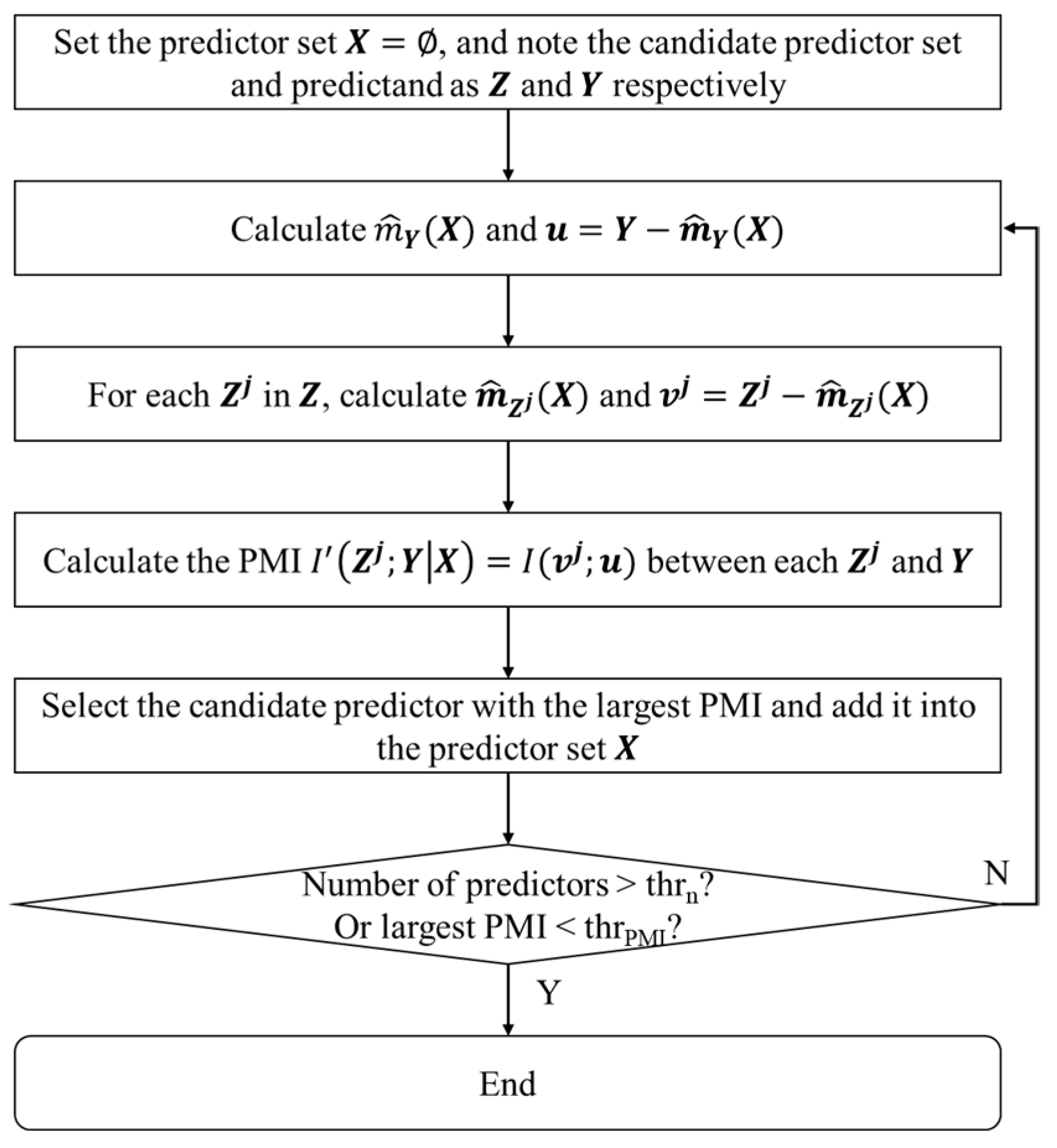
2.1.1. The Predictor Selection Method

Predictor selection is a process applied to recognize the most valuable predictors from numerous candidate predictors in order to reduce the model’s complexity and improve its accuracy [56,59]. Among many predictor selection methods, the MI can reflect the nonlinear relationship and is used in this study. The selection method based on MI is briefly described as follows, and details can be found in other studies [55,60,61].

For the prediction Y and candidate predictors X, the MI is defined as follows:

$$I\left(\mathit{X};\mathit{Y}\right)=\int \int p\left(x,y\right)\log \frac{p\left(x,y\right)}{p\left(x\right)p\left(y\right)}dx dy$$

(1)

where $p\left(x\right)$ and $p\left(y\right)$ represent the marginal probability density functions (pdfs) of X and Y, and $p\left(x,y\right)$ is the joint pdf. In the application, the MI can be obtained by a numerical approximation as follows:

$$I\left(\mathit{X};\mathit{Y}\right)=\frac{1}{n}\sum _{i=1}^n\log \frac{f\left(x_i,y_i\right)}{f\left(x_i\right)f\left(y_i\right)}$$

(2)

where f denotes the estimated density based on a sample of n observations of (x, y), and can be estimated with the kernel density estimation (KDE):

$$\widehat{f}\left(x\right)=\frac{1}{n}\sum _{i=1}^n{K}_h\left(x-x_i\right)$$

(3)

where $\widehat{f}\left(x\right)$ denotes the estimate of the pdf at $x$; $x_i$ denote the ith observation of X; and $K_h$ is some kernel function for which a common choice is the Gaussian kernel.

The MI can be used to evaluate the correlation between predictand and predictors, but it cannot identify the internal relation among the predictors and may cause redundant information in the predictors [61]. Therefore, the partial mutual information (PMI), which quantifies the nonlinear dependence of Y on the candidate predictor Z that is not accounted for by the selected predictor X, is introduced. The PMI is calculated by first filtering both Y and Z via regression on X to obtain residuals u and v, respectively:

$$\mathit{u}=\mathit{Y}-{\widehat{\mathit{m}}}_{\mathit{Y}}\left(\mathit{X}\right)$$

(4)

$$\mathit{v}=\mathit{Z}-{\widehat{\mathit{m}}}_{\mathit{Z}}\left(\mathit{X}\right)$$

(5)

where ${\widehat{\mathit{m}}}_{\mathit{Y}}\left(\mathit{X}\right)$ and ${\widehat{\mathit{m}}}_{\mathit{Z}}\left(\mathit{X}\right)$ represent the estimators for the regression of Y and Z on X. Based on the KDE, the ${\widehat{\mathit{m}}}_{\mathit{Y}}\left(\mathit{X}\right)$ can be written as:

$${\widehat{\mathit{m}}}_{\mathit{Y}}\left(\mathit{X}\right)=E\left[y|\mathit{X}=x\right]=\frac{1}{n}\frac{{\sum }_{i=1}^n{y}_i{K}_h\left(x-x_i\right)}{{\sum }_{i=1}^n{K}_h(x-x_i)}$$

(6)

Then, the PMI can be calculated by:

$$I^{\prime }\left(\mathit{Z};\mathit{Y}|\mathit{X}\right)=I(\mathit{v};\mathit{u})$$

(7)

Based on the previous equations, the process of the predictor selection method based on the MI and PMI, named PMIS, is showed in Figure 1. The $th{r}_n$ and $th{r}_{PMI}$ are thresholds.

2.1.2. Total Mutual Information

The PMIS can be proposed to select suitable predictors from numerous candidate variables, but the PMI cannot reflect the relation between the whole predictor set and the prediction, and the MI cannot reflect the internal relationship among the predictor set. Therefore, the total mutual information (TMI) is developed based on the PMIS method to reflect the relation between the whole predictor set and the prediction. The TMI can be calculated using the following equation:

$$\mathrm{T}\mathrm{M}\mathrm{I}=\sum _{i=1}^m{w}_i{\mathrm{P}\mathrm{M}\mathrm{I}}_i$$

(8)

where $m$ is the number of selected predictors; $i$ is the order of selecting the predictor; and $w_i$ and ${\mathrm{P}\mathrm{M}\mathrm{I}}_i$ are the weight and PMI value of the ith selected predictor.

The $w_i$ can be determined by calculating the information gained after introducing the specific predictor. Considering that the residual shown in Equation (4) can represent the uncertainty in the prediction to some degree, the difference in the standard deviation of the residual is used to represent the information gained. Then, the $w_i$ can be calculated as follows:

$$w_i=\mathrm{s}\mathrm{t}\mathrm{d}\left(\mathit{Y}-{\widehat{\mathit{m}}}_{\mathit{Y}}\left({\mathit{X}}^{\mathit{i}-1}\right)\right)-\mathrm{s}\mathrm{t}\mathrm{d}\left(\mathit{Y}-{\widehat{\mathit{m}}}_{\mathit{Y}}\left({\mathit{X}}^{\mathit{i}}\right)\right)$$

(9)

where ${\mathit{X}}^{\mathit{i}}$ represents the predictor set after introducing the ith predictor and std denote the standard deviation.

2.2. Case Study and Data Preparing

In order to analyze the relationship between the TMI and the predictive performance of MLTRP, predictions were generated at 37 hydrologic reference stations in Australia selected from 221 stations. The station selection occurred according to two criteria: (1) the data quality, as evaluated by the Bureau of Meteorology (BOM) in Australia, is the “best available data”; and (2) the starting month of the data is earlier than January 1966. All stations were located in catchments with minimal anthropogenic interruptions. The 37 stations and corresponding catchments are shown in Figure 2, and the basic information is listed in Appendix A.

The monthly runoff data of the 37 selected stations can be obtained from the website of BOM, Australia (http://www.bom.gov.au/water/hrs/, accessed on 1 January 2021). The available runoff records all end in December 2014, and the starting months at different stations are between January 1951 and July 1982. In order to process the skewness in runoff data, the runoff data were preprocessed using a widely used log-sinh data transformation method [58,62,63]. And it should be noted that the following results are demonstrated and discussed based on the transformed data in order to compare the model’s predictive performances in different basins.

The other data used in this study include rainfall and 130 global climate factors. The grid rainfall data with 0.05° resolution were obtained through Australian Water Availability Project (http://www.auscover.org.au/purl/australian-gridded-climate-data, accessed on 1 January 2021) and processed to obtain the monthly rainfall in the area. The 130 global climate factors data, including 88 atmospheric circulation indices, 26 SSTA indices, and 16 other indices, were downloaded from the website of National Climate Center, China Meteorological Administration (http://cmdp.ncc-cma.net/en/, accessed on 1 January 2021). The climate data were normalized by:

$${\widehat{F}}_{year,month}=\frac{F_{year,month}-{\overline{F}}_{month}}{S_{month}}$$

(10)

where $F$ is the original data, $\widehat{F}$ is the transformed data, year and month represent time, $\overline{F}$ is the mean value, and $S$ is the standard deviation.

2.3. Forecasting Models and Model Development Process

2.3.1. Forecasting Models

Five AI models were used to generate mid-to-long-term runoff predictions in this study. The five models were the multilayer perceptron (MLP) model, the block-based MLP (MB) model, the Bayesian SVR (BSVR) model, a coupled BSVR and ARD kernel model (BSVRARD), and the LSTM model. Because these five models have been widely used in many fields, their details are not introduced in this study and can be found in other previous studies [24,56,64,65,66,67]. The features of these five models are briefly summarized in

Table 1. Brief introduction of five models applied in this study.

Model	Introduction
MLP	Commonly used three-layer neural network.
MB	Based on the MLP, a block data structure is used to incorporate the time series information. The details of this method can be found in [56].
BSVR	A model in which the Bayesian inference framework is used to optimize the parameters of SVR. The details can be found in [64,65,66].
BSVRARD	A model integrating the BSVR and ARD kernel. The details can be found in [64,65,66].
LSTM	Commonly used deep learning neural network which is suitable for time series forecasting. The details of LSTM can be found in [67].

.

The MLP model is the most widely used ANN model in many fields, and is used in this study to establish a relationship between the input vector X_t, which includes the values of selected predictors at a specific time t, and output value Y_t, which is the value of prediction (i.e., the monthly runoff). Similarly to the MLP model, the BSVR model is also used to establish the X_t-Y_t relationship. But the BSVR and MLP models have different model structures and parameters, which can be found in some previous studies [16,51,64,65,66,68]. Based on the BSVR model, the BSVRARD model proposed the ARD kernel to discriminate the importance of predictors [64,65,66]. Compared with the MLP, BSVR, and BSVRARD models, the MB and LSTM models focus more on the time series information, and they are used to establish the relationship between the input matrix [X_t−m, …, X_t−1, X_t], which includes the time series values of selected predictors in a time range t − m and t, and the output value Y_t [56]. The MB was developed by integrating the MLP model and the block structure, and the LSTM model was developed based on the recurrent model [56,69]. The MB and LSTM models mainly differ in terms of model structure and ability to process input information. In general, the MLP, BSVR, and BSVRARD models focus more on the point information at a specific time, and the MB and LSTM models focus more on the time series information in a specific time range.

2.3.2. Model Development Process

The commonly used model development process introduced in [56,57] is proposed and modified in this study. Firstly, the PMIS method was used to select predictors and organized to meet the input format requirement of the five models. Meanwhile, the TMI and MI were calculated along with the PMIS process. Secondly, leave-one-year-out cross-validation was applied in this study to generate predictions using the whole dataset of each station. Thirdly, the five models were constructed and validated.

The validation metrics included: (1) root mean square error (RMSE) and (2) relative root mean square error (RRMSE). The two metrics were calculated according to the following equations.

$$\mathrm{R}\mathrm{M}\mathrm{S}\mathrm{E}=\sqrt{\frac{1}{n}{\sum }_{i=1}^n{\left({\widehat{Y}}_i-Y_i\right)}^2}\hspace{1em}\in [0,+\mathrm{\infty })$$

(11)

$$\mathrm{R}\mathrm{R}\mathrm{M}\mathrm{S}\mathrm{E}=\frac{\mathrm{R}\mathrm{M}\mathrm{S}\mathrm{E}}{{\sigma }_{\mathit{Y}}}\hspace{1em}\in [0,+\mathrm{\infty })$$

(12)

where ${\widehat{Y}}_i$ and $Y_i$ are the predicted and observed values, respectively; $N$ is the number of validation data; and ${\sigma }_{\mathit{Y}}$ is the standard error.

Because the ${\sigma }_{\mathit{Y}}$ can represent the predictive performance of a model using the average values as predictions (named average model), the RRMSE, which is the ratio of the RMSE of a specific model to ${\sigma }_{\mathit{Y}}$, can represent the forecasting model’s applicability to some degree. A RRMSE value larger than 1 means that the model’s predictive performance is worse than the average model and cannot generate valuable predictions.

2.4. Experiment Setup

In order to examine the ability of TMI to evaluate the applicability of MLTRP, two experiments were implemented in this study and are summarized in

Table 2. Experiment setup.

Experiment	Candidate Predictors	Prediction	Validation Metrics	Evaluation Indices	Analysis
Experiment 1 (E1)	130 climate factors and transformed runoff in the previous 12 months.	Runoff of the 37 stations in the future 1–6 months. In total 37 × 6 = 222 forecasting scenarios.	RMSE, RRMSE.	MI and TMI.	The relationships of RMSE-TMI, RRMSE-TMI, and RRMSE-MI.
Experiment 2 (E2)	The candidate predictors in E1 and rainfall in the previous 12 months and future FLT (forecast lead time) months.	Runoff of the 37 stations in the future 1–6 months. In total 37 × 6 = 222 forecasting scenarios.	RMSE, RRMSE.	MI and TMI.	The relationships of RMSE-TMI, RRMSE-TMI, and RRMSE-MI.

. The main difference in the two experiments was the candidate predictor set. In experiment 1 (E1), the candidate predictions included 130 climate factors and transformed runoff in the previous 12 months. In experiment 2 (E2), the candidate predictors included those in the E1, as well as area rainfall in the previous 12 months and future FLT (forecast lead time) months. Based on the candidate predictors, five AI models were used to predict runoff of the 37 stations in the future 1–6 months (37 × 6 = 222 forecasting scenarios), and RMSE and RRMSE were used to evaluate the predictive performance. Meanwhile, the MI and TMI were calculated. Finally, the relationships of RMSE-TMI, RRMSE-TMI, and RRMSE-MI were analyzed. In addition, the TMI and predictive performance were further compared between the two experiments.

3. Results

The results of the five forecasting models without and with rainfall in candidate predictors (i.e., E1 and E2) are presented in terms of the RMSE and RRMSE in Section 3.1 and Section 3.2, respectively.

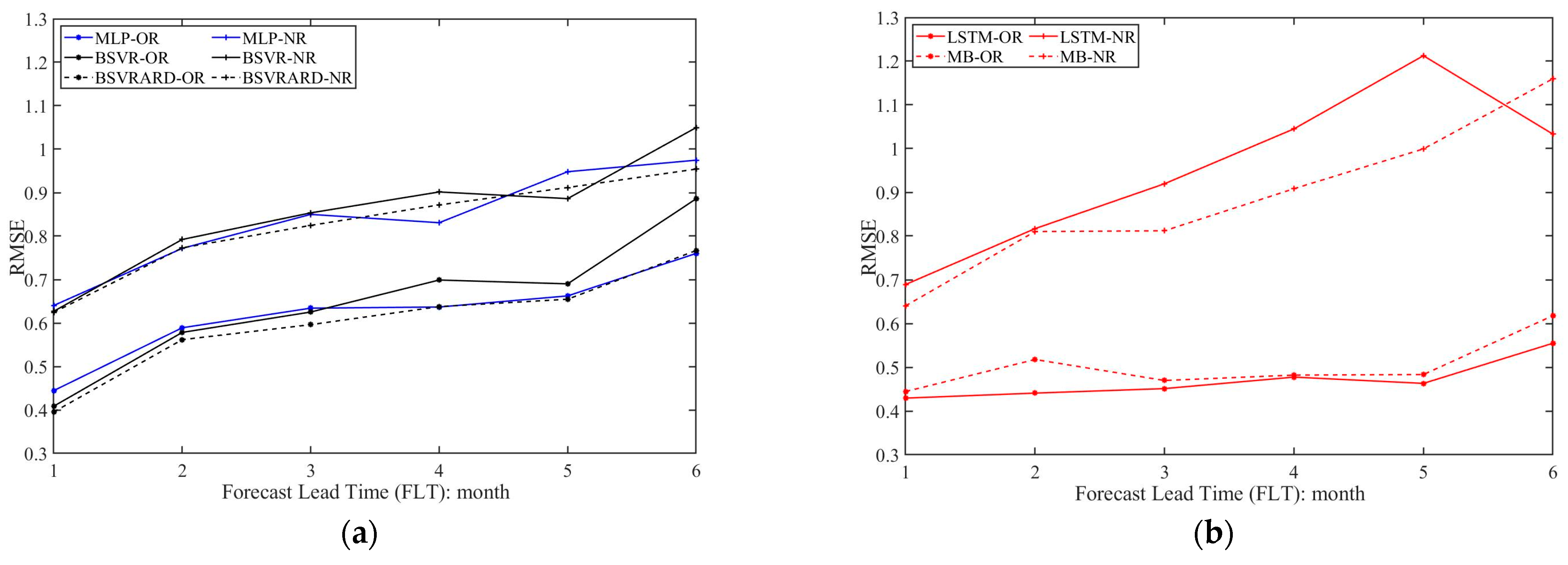
3.1. The Predictive Performance of Five Models without Rainfall in Predictors

The cross-validated predictive performances of the five AI models (i.e., MLP, LSTM, MB, BSVR, and BSVRARD) were examined using the root mean square error (RMSE) and relative root mean square error (RRMSE) obtained for the validation data, as shown in Figure 3. In the figure, the x-axis and y-axis represent the FLT and station ID, and the colors represent the RMSE and RRMSE values. The difference in predictive performance resulted from the differences among basins, FLTs, and models. It can be seen from Figure 3 that the difference in predictive performance caused by the difference in basins was the most significant. In addition, the basins with smaller RMSE values and the basins with smaller RRMSE values were different due to the characteristics of the transformed runoff time series. In terms of the influence of the FLT, it can be seen that the all model will obtain best predictive performance, which will become worse along with the increase of FLT. In general, it is obvious that the difference in predictive performance caused by the difference in forecasting scenarios (different basins and different FLTs) was more significant than that caused by the models.

3.2. The Predictive Performance of Five Models with Rainfall as Predictor

The cross-validated predictive performances of the five AI models were examined using the RMSE and RRMSE obtained over the validation data with rainfall as a predictor, as shown in Figure 4. It can be seen that the RMSE values of the 222 forecasting scenarios (37 stations × 6 FLTs) were within 0.4–2.3 and significantly decreased compared with those obtained in experiment 1 (E1, without rainfall as predictors), as shown in Figure 3. And the RRMSE values decreased from 0.35–1.25 (Figure 3) to 0.2–0.85 (Figure 4). In addition, the difference in predictive performance among the different basins was still significant. In terms of the influence of FLTs on predictive performance, different models showed different features, which can be seen from Figure 5. In E2, where the observed rainfall was included as a predictor, the predictive performance became significantly worse for the MLP, BSVR, and BSVRARD models (i.e., point models) along with the increase in FLTs, which can be seen in Figure 5a. But the predictive performances of the time series models (i.e., MB and LSTM) were steadier among different FLTs, which can be seen in Figure 5b. In E1, the predictive performances of all models showed similar trend with the increase in FLT. Although the LSTM and MB models performed worse in E1, the two models had better performances after the incorporation of rainfall (E2). In addition, the advantages of the time series models (MB and LSTM) compared with the point models (MLP, BSVR and BSVRARD) were more obvious along with the increase in FLT.

4. Discussion

The results are discussed in this section. First, the five models are compared in terms of the predictive performance in Section 4.1. Second, the relationship between the total mutual information (TMI) and the predictive performance of five models is analyzed in Section 4.2. Finally, the influence of the incorporation of rainfall on the predictive performance is discussed in Section 4.3.

4.1. The Comparison of Different Models

The predictive performance of the five models (i.e., MLP, LSTM, MB, BSVR, and BSVRARD) in terms of the RRMSE in 222 forecasting scenarios (37 stations × 6 FLTs) without rainfall as a predictor (E1) is illustrated in Figure 6a, and that of E2 is illustrated in Figure 6b. In Figure 6, the y-axis shows the values of the RRMSE, and the x-axis shows the number of forecasting scenarios with RRMSE below specific values. It can be seen from Figure 6a that in the three neural network models (MLP, LSTM and MB), the MLP model performed best, and the LSTM model performed worst. Though the LSTM models showed better performances than the simple machine learning models in many fields, such as flood prediction and rainfall–runoff modelling, some studies have also demonstrated that the effect of LSTM depends on the available data [23,56,70]. In MLTRP, the data are all monthly runoff, and the limited data may be not enough to support the application of the LSTM model. Furthermore, the LSTM is widely used in short-term runoff prediction, where the prediction (runoff) has a clear physical correlation with the predictors (rainfall and temperature). But in this study, the forecasting models were constructed based on the teleconnection between monthly runoff and climate factors in E1, where rainfall was not included as a predictor. Due to both the limited data and the weak connection between the predictors and the prediction in the MLTRP, the most complex LSTM model performed worst, and the complex MB model was worse than the MLP model. But the opposite result was obtained in E2, as shown in Figure 6b. It is obvious that the LSTM and MB models performed significantly better than the other three models (i.e., MLP, BSVR, and BSVRARD). The main difference between E1 and E2 was that the rainfall was incorporated into the predictors. After the application of rainfall, there was strong physical connection between the predictors and the prediction. This means that the complex models, which were able to use the time series information, performed better. In terms of the comparison among the three point models (MLP, BSVR, and BSVRARD), the BSVR and BSVRARD models performed better than the MLP model because the uncertainty risks of the model structure and parameters were incorporated in the SVR model, and the solution of the SVR model was globally optimized [71].

4.2. The Relationship between Predictive Performance and TMI, MI

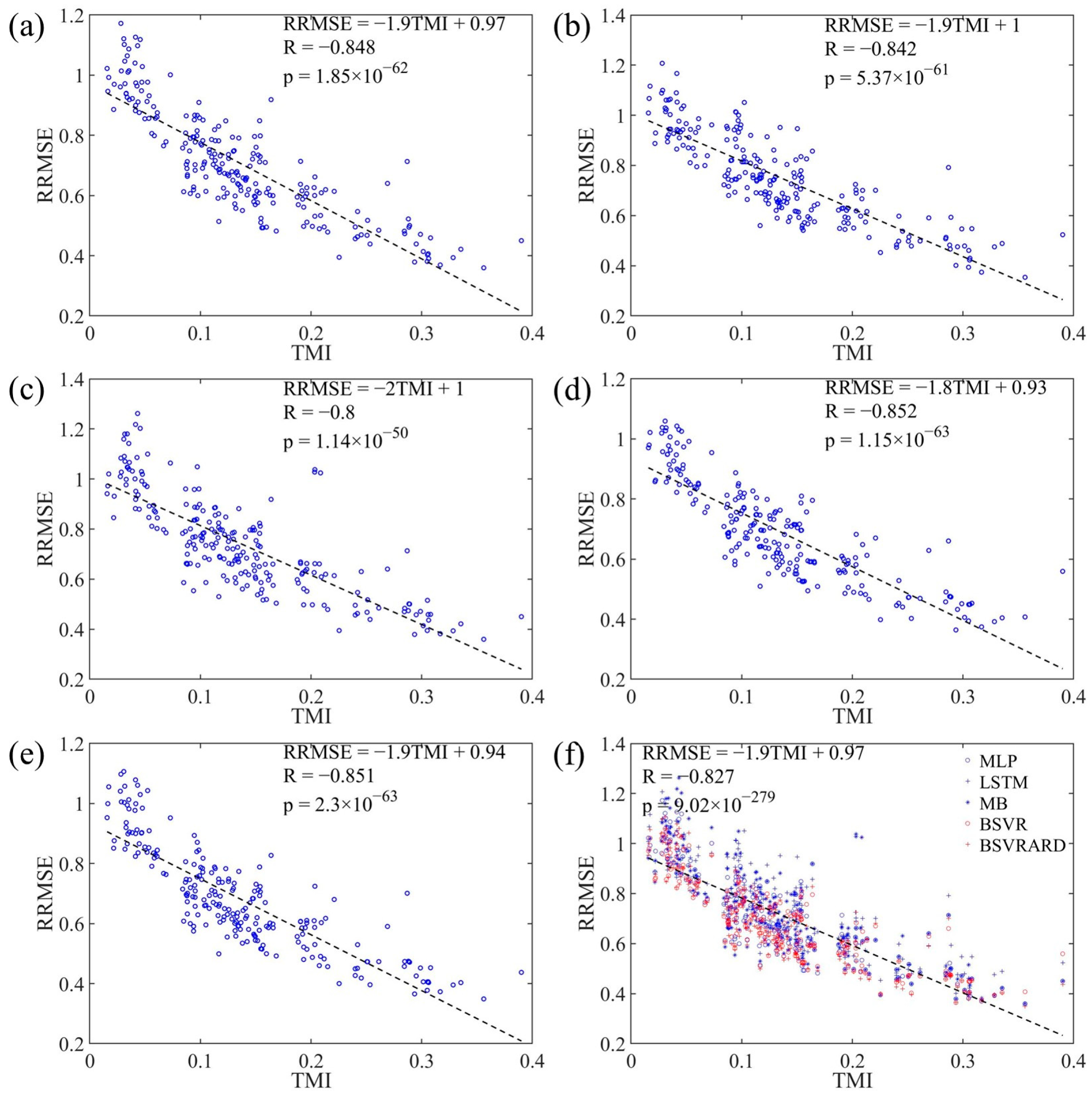
4.2.1. RRMSE and MI in E1

The RRMSE values of 222 forecasting scenarios and the corresponding MIs are shown in Figure 7, where the linear regression equation and p values are also illustrated. It can be seen that there is a good linear correlation relationship with the correlation coefficient around −0.6 and a p value less than 4.53 × 10⁻²¹. This means that there is a close connection between the predictive performance and the available information in the predictors, which can be represented by the MI. Even if the RRMSE and MI values are combined in Figure 7f, there is still a good linear correlation relationship. This means that the predictive performance difference caused by the model’s difference is not significant compared with that caused by the difference among MIs. The overall linear regression equation is RRMSE = −0.65 × MI + 1.2, which means that the RRMSE is 1.2, showing that the model is worse than an average model when the MI is zero. Although the MI can represent the available information in the predictors to some degree, and there is a good correlation between RRMSE and MI, the correlation is not very significant and needs to be further improved.

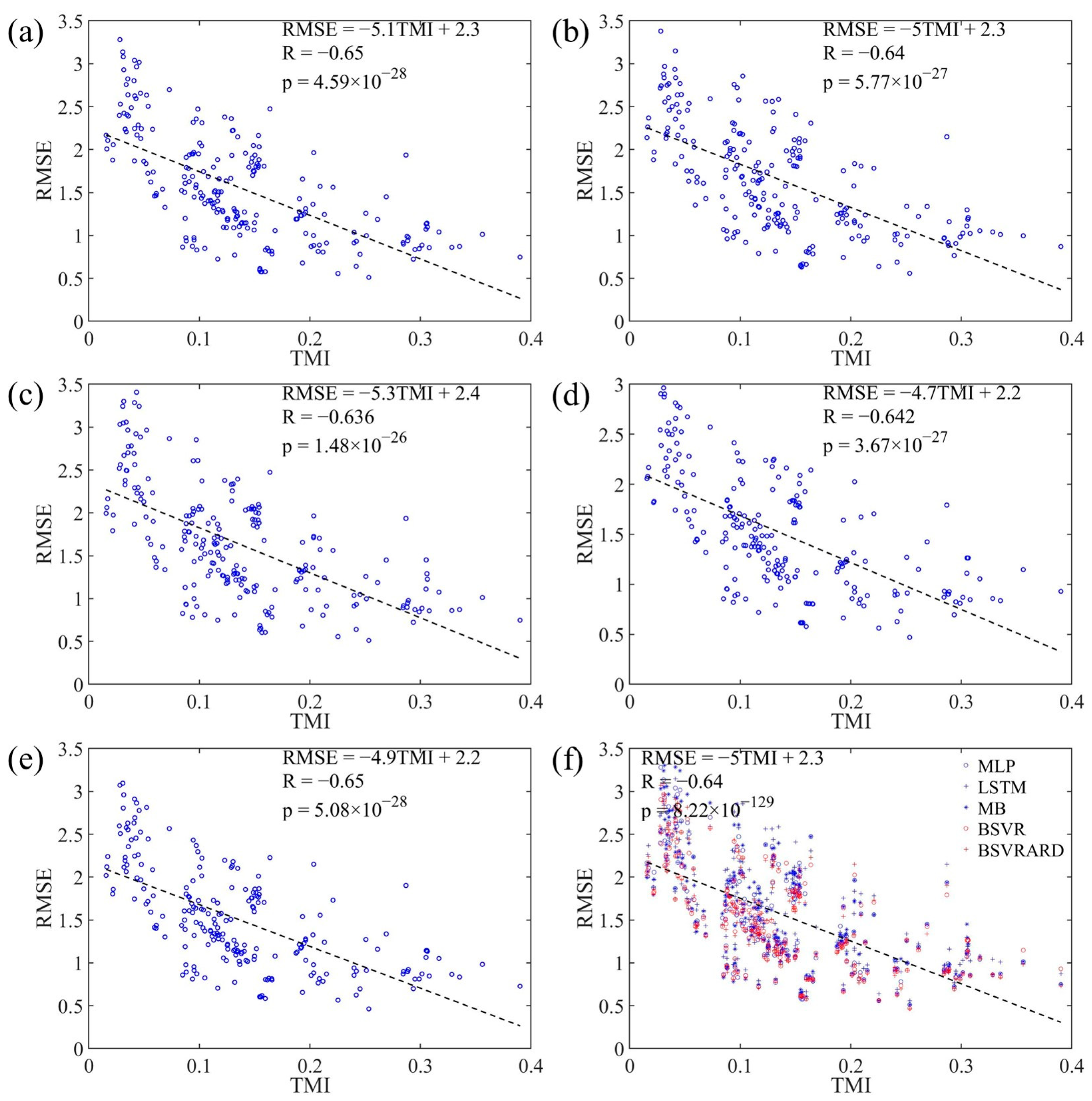
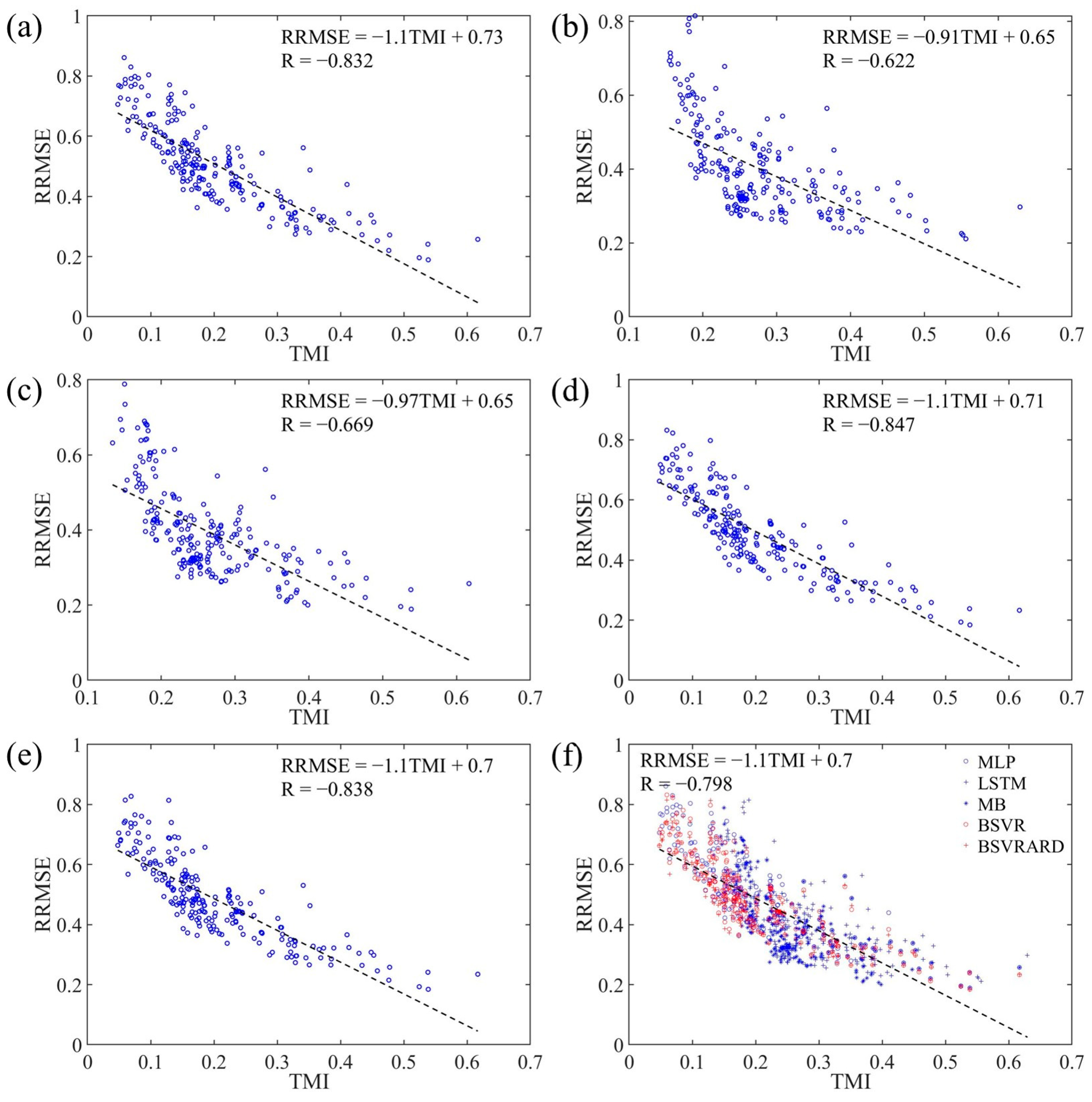
4.2.2. RMSE, RRMSE and TMI

The RRMSE and RMSE values of 222 forecasting scenarios and the corresponding TMIs are shown in Figure 8 and Figure 9, respectively. It is clear that the RMSE has a negative correlation with the TMI, and the correlation coefficient is around −0.65, with a p value less than 1.48 × 10⁻²⁶. However, the RMSE in affected not only by the available information in the predictors (TMI and MI), but also the statistical characteristics of the transformed runoff time series. Therefore, the RRMSE, which is calculated through dividing the RMSE by the standard deviation of the time series, has a stronger negative correlation with the TMI, which can be seen in Figure 8. The correlation coefficients are between −0.8 and −0.85, with p values less than 1.14 × 10⁻⁵⁰. Compared with the correlation coefficients of RRMSE-MI (Figure 7) and RMSE-TMI (Figure 9), the correlation coefficients of RRMSE-TMI are closer to −1. This means that the TMI can better represent the available information regarding the predictors compared with the MI. The main difference between the MI and TMI is the way to discriminate the predictors. The MI is used to evaluate the mutual information between all predictors and the prediction, but it cannot discriminate the importance of the predictors. The TMI is calculated by multiplying the PMIs of predictors with weights which represent the information gained after incorporating the predictor. Therefore, the TMI can discriminate the predictors and better represent the available information.

Because the TMI can represent the available information in the predictors and has a strong correlation with the predictive performance, the TMI can be used to evaluate the applicability of MLTRP in a specific forecasting scenario. If the TMI is smaller, it is inappropriate to make mid-to-long-term runoff predictions using data-based models. It can be seen from Figure 8 that the RRMSE values of almost all models were less than 1 when the TMI was more than 0.1. This means the model can generate valuable forecasting information compared with the average model using average values as predictions. When the TMI is less than 0.1, the RRMSE may be more than 1 in some forecasting scenarios. In addition, considering the linear regression equation RRMSE = −1.9 TMI + 0.97, the corresponding RRMSE is 0.78 with TMI equal to 0.1, which means that the predictive performance is good.

In general, the predictive performance shows a strong correlation with the TMI, which represents the available information in the predictors, and therefore, the TMI can be used to evaluate the applicability of MLTRP. A TMI of more than 0.1 may represent that the corresponding forecasting scenario is suitable for applying a data-based model to generate valuable predictions.

4.2.3. The Linear Regression Equations between RRMSE and MI and TMI

The linear regression equations between RRMSE and MI and TMI are shown in Figure 8 and Figure 9, and the slopes and intercepts are summarized in

Table 3. The slopes and intercepts of linear regression equations between RRMSE and MI and TMI.

Independent Variable		Model
		MLP	LSTM	MB	BSVR	BSVRARD	All
MI	Slope	−0.665	−0.638	−0.681	−0.620	−0.654	−0.652
	Intercept	1.192	1.215	1.240	1.142	1.159	1.190
TMI	Slope	−1.937	−1.907	−1.976	−1.787	−1.862	−1.894
	Intercept	0.970	1.008	1.011	0.932	0.935	0.972

. It can be seen that the intercepts were around 1.2 when MI was the independent variable and around 1 when TMI was the independent variable. When the predictor set was empty, the MI and TMI were 0, and the fitted RRMSE values were 1.2 and 1, respectively. Meanwhile, the forecasting results show be the average values of the time series and the real RRMSE of forecasting model should be 1. From this perspective, the TMI can better represent the predictive performance.

It can also be seen from Table 3 that the slopes and intercepts for different models different significantly. The difference in slopes can partly explain the differences in the five models. A lower slope value (larger absolute value) means that the model was more sensitive to the available information regarding the predictors. It is obvious that the slopes of the two time series models (MB and LSTM) were less than those of the two SVR models (point models). The underlying reason is the difference among model characteristics. The MB and LSTM models have more complex structures and can utilize information better [56]. Therefore, when the available information contained in the predictors increased, which can be reflected by the increase in TMI, the predictive performances of the MB and LSTM models became better and faster, which is reflected in the lower slope values. This can also explain the differences in intercepts. When TMI was equal to 0, the available information was limited and could not support the establishment of the complex models (MB and LSTM); thus, the MB and LSTM models performed worse, which is reflected by the larger intercept values. It should be noted that the MLP model had a significantly smaller slope than the two SVR models, although the MLP model’s structure is simple and similar to the SVR model. The underlying reason is that the MLP model may fall into local optima and has unstable predictive performance in different forecasting cases.

4.3. The Influence of Rainfall on the Predictive Performance and TMI

In E2, where the rainfall was included as a predictor, five models’ predictive performances became significantly better, which may be reflected by the change in TMI. Therefore, the RRMSE and TMI values in E2 were calculated and are shown in Figure 10. It can be seen from Figure 10 that the TMI values were between 0.05 and 0.65 and the RRMSE values were between 0.2 and 0.9 after incorporating the rainfall into the predictor set. Compared with the results obtained without rainfall as a predictor (Figure 8), the TMI values increased by 0.01–0.31 and the corresponding RRMSE decreased by −0.01–0.69. It can also be seen from Figure 10 that the RRMSE leveled off along with the increase in TMI.

After the incorporation of rainfall, the five models showed different features. For the LSTM and MB models, the TMI values were all more than 0.1, and the RRMSE values were less than 0.8. But for the MLP, BSVR, and BSVRARD models, there were still 13.5 forecasting scenarios where the TMI was less than 0.1 and the RRMSE values were around or more than 0.8. The reason for the difference in TMI among the five models is that the time series information was used in the LSTM and MB models.

It can be seen from Figure 10 that there was still a significant negative correlation between the RRMSE and TMI. For the three-point models (MLP, BSVR, and BSVRARD), the correlation coefficients were around −0.83. But for the LSTM and MB models, the correlation coefficients were −0.62 and −0.67, respectively. The difference in the five models in terms of the coefficients was caused by the difference among the models’ structures. The LSTM and MB models use time series data as model input. But time series characteristics are not considered in the calculation of PMIS, and therefore, the TMI can only partly explain the available information in the input time series data. Nevertheless, the overall correlation coefficient for all five models was −0.80.

Besides the rainfall, the soil moisture, the vegetation condition, the land cover, and many other factors influence the runoff by affecting the rainfall–runoff process [19,72,73]. For example, the antecedent soil moisture may influence the runoff yield significantly [72,73]. From the perspective of runoff prediction, the antecedent soil moisture and the land cover can be added into the predictor set to increase the TMI and improve the predictive performance, which can be investigated in a future study.

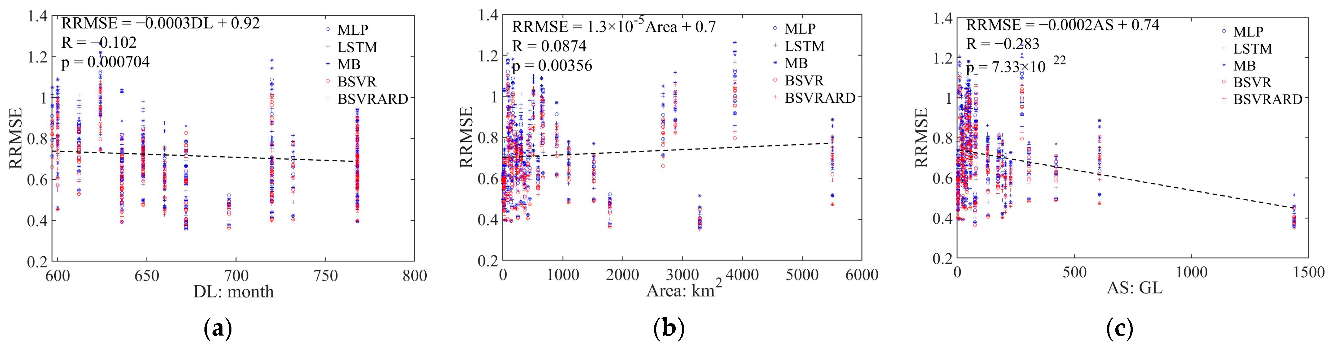
4.4. The Impact Factors of Predictive Performance

The TMI is a statistical indicator which has a significant correlation with the predictive performance, but it is not the physical root cause for the differences in predictive performance. Therefore, the physical impact factors of predictive performance are analyzed in this section.

After the incorporation of rainfall, the TMI values increase in most forecasting cases. However, the increase in TMI values and the improvement of predictive performance are not significant in some basins. For example, for the No. 36 station, the increase in TMI was 0.01, which means the information gained by using the rainfall factor was not significant. In order to analyze the reason, the rainfall–runoff in relation to the transformed data is plotted in Figure 11. It is obvious that the transformed runoff had a significant positive correlation with the rainfall. However, when the runoff was near 0 (the line at the bottom of Figure 11), the rainfall was not 0, which means that the rainfall did not yield runoff in these months. The underlying reason may be the difference between the real rainfall and “observed” rainfall in some small basins. In this study, the observed rainfall was obtained from the interpolated gridded rainfall data provided by the Australian Water Availability Project. In some small basins, the interpolated rainfall used in this study did not reflect the real situation, and therefore, the incorporation of rainfall cannot provide much information.

Besides the area, the available data length (DL) and the annual average streamflow (AS) may also affect the predictive performance [27,56,57]. The relationship between the predictive performance (RRMSE) and the area, DL, and AS can be seen in Figure 12. It is clear that the area, DL, and AS may influence the predictive performance, and generally, the predictive performance will become better in larger basins with greater annual average streamflows and longer data lengths. However, the correlation coefficients between the RRMSE and these three factors were near 0, and the correlation was not significant with the relatively large p-values for the DL and area. The reason is that the predictive performance in a specific forecasting case is affected by multiple factors which can influence the available information in the predictor set, and these factors cannot individually explain the differences in predictive performance in different forecasting cases. But the comprehensive impact of these factors on the predictive performance cannot be assessed quantitatively, and therefore, they cannot be used to evaluate whether there will be a good predictive performance in a specific forecasting case. Against this background, the TMI index is developed. The TMI index can represent the comprehensive impact of multiple factors to some degree due to its ability to reflect the available information in the predictor set, and therefore, it can explain the differences in predictive performance among different forecasting cases more effectively compared with these factors.

5. Conclusions

In this study, the total mutual information (TMI) index is developed based on the predictor selection method called PMIS, which recognizes predictors based on the mutual information (MI) and partial MI (PMI). In order to examine the relationship between the TMI and the predictive performance, five AI models (MLP, LSTM, MB, BSVR, and BSVRARD) are applied at 37 hydrological stations in Australia to predict monthly runoff in the future 1–6 months, and the RMSE and RRMSE are used to evaluate the predictive performance in 222 forecasting scenarios. The relationship of TMI, RMSE, and RRMSE in two different experiments is assessed with and without the application of rainfall. The main conclusions are as follows:

(1)

The developed TMI index can represent the available information in the predictors better than the MI index, and has a significant negative correlation with the RRMSE. The correlation coefficients are between −0.8 and −0.85 when the rainfall is not included as a predictor. And when the rainfall is included as a predictor, the coefficients are between −0.62 and −0.85.

(2)

The developed TMI index can be used to evaluate the applicability of MLTRP. Along with the increase in TMI, the available information increases and the model’s predictive performance becomes better. When the TMI is more than 0.1, the available information of the predictors can support the construction of MLTRP models, and the model can generate valuable predictions. When the TMI is less than 0.1 and near 0, the MLTRP may be not suitable in the forecasting scenarios.

(3)

The five AI models have significantly different performances in different scenarios. When the rainfall is not included as a predictor, the complex LSTM and MB models using time series as inputs perform worse than the MLP, BSVR, and BSVRARD models. After the incorporation of rainfall as a predictor, the TMI increases significantly, and the complex LSTM and MB models, which can better utilize the contained information in the predictors, perform better than the other three models.

(4)

The differences in the five models can be partly explained by the developed TMI index. The slopes of the linear regression equation between the RRMSE of the LSTM and MB models and the TMI are less than those for the BSVR and BSVRARD models. This means the LSTM and MB models are more sensitive to the available information of the predictors (i.e., TMI), and therefore, the changes in the predictive performance for the LSTM and MB models are more significant than that of the BSVR and BSVRARD models after the incorporation of rainfall as a predictor.

(5)

The developed TMI index is just a statistical indicator reflecting the available information in the predictor set, which affects the predictive performance of data-driven models, but the root cause for the difference in predictive performance is the characteristics of the basin.

References

1. Nguyen, Q.H.; Tran, V.N. Temporal Changes in Water and Sediment Discharges: Impacts of Climate Change and Human Activities in the Red River Basin (1958–2021) with Projections up to 2100. Water 2024, 16, 1155. [Google Scholar] [CrossRef]
2. Jia, L.; Niu, Z.; Zhang, R.; Ma, Y. Sensitivity of Runoff to Climatic Factors and the Attribution of Runoff Variation in the Upper Shule River, North-West China. Water 2024, 16, 1272. [Google Scholar] [CrossRef]
3. Xu, H.; Liu, L.; Wang, Y.; Wang, S.; Hao, Y.; Ma, J.; Jiang, T. Assessment of climate change impact and difference on the river runoff in four basins in China under 1.5 and 2.0 °C global warming. Hydrol. Earth Syst. Sci. 2019, 23, 4219–4231. [Google Scholar] [CrossRef]
4. Zou, L.; Zhou, T. Near future (2016–40) summer precipitation changes over China as projected by a regional climate model (RCM) under the RCP8.5 emissions scenario: Comparison between RCM downscaling and the driving GCM. Adv. Atmos. Sci. 2013, 30, 806–818. [Google Scholar] [CrossRef]
5. Piao, S.L.; Ciais, P.; Huang, Y.; Shen, Z.H.; Peng, S.S.; Li, J.S.; Zhou, L.P.; Liu, H.Y.; Ma, Y.C.; Ding, Y.H.; et al. The impacts of climate change on water resources and agriculture in China. Nature 2010, 467, 43–51. [Google Scholar] [CrossRef] [PubMed]
6. Larraz, B.; García-Rubio, N.; Gámez, M.; Sauvage, S.; Cakir, R.; Raimonet, M.; Pérez, J.M.S. Socio-Economic Indicators for Water Management in the South-West Europe Territory: Sectorial Water Productivity and Intensity in Employment. Water 2024, 16, 959. [Google Scholar] [CrossRef]
7. Haj-Amor, Z.; Acharjee, T.K.; Dhaouadi, L.; Bouri, S. Impacts of climate change on irrigation water requirement of date palms under future salinity trend in coastal aquifer of Tunisian oasis. Agric. Water Manag. 2020, 228, 105843. [Google Scholar] [CrossRef]
8. Shukla, P.R.; Skeg, J.; Buendia, E.C.; Masson-Delmotte, V.; Pörtner, H.O.; Roberts, D.C.; Zhai, P.; Slade, R.; Connors, S.; Van Diemen, S.; et al. Climate Change and Land: An IPCC Special Report on Climate Change, Desertification, Land Degradation, Sustainable Land Management, Food Security, and Greenhouse Gas Fluxes in Terrestrial Ecosystems; IPCC: Geneva, Switzerland, 2019. [Google Scholar]
9. Bărbulescu, A.; Zhen, L. Forecasting the River Water Discharge by Artificial Intelligence Methods. Water 2024, 16, 1248. [Google Scholar] [CrossRef]
10. Chu, H.; Wei, J.; Wu, W. Streamflow prediction using LASSO-FCM-DBN approach based on hydro-meteorological condition classification. J. Hydrol. 2020, 580, 124253. [Google Scholar] [CrossRef]
11. Xie, S.; Huang, Y.F.; Li, T.J.; Liu, C.Y.; Wang, J.H. Mid-long term runoff prediction based on a Lasso and SVR hybrid method. J. Basic Sci. Eng. 2018, 26, 709–722. [Google Scholar]
12. Feng, Z.-K.; Niu, W.-J.; Tang, Z.-Y.; Jiang, Z.-Q.; Xu, Y.; Liu, Y.; Zhang, H.-R. Monthly runoff time series prediction by variational mode decomposition and support vector machine based on quantum-behaved particle swarm optimization. J. Hydrol. 2020, 583, 124627. [Google Scholar] [CrossRef]
13. Sunday, R.; Masih, I.; Werner, M.; van der Zaag, P. Streamflow forecasting for operational water management in the Incomati River Basin, Southern Africa. Phys. Chem. Earth Parts A/B/C 2014, 72, 1–12. [Google Scholar] [CrossRef]
14. Shamir, E. The value and skill of seasonal forecasts for water resources management in the Upper Santa Cruz River basin, southern Arizona. J. Arid. Environ. 2017, 137, 35–45. [Google Scholar] [CrossRef]
15. Zhao, H.; Li, H.; Xuan, Y.; Bao, S.; Cidan, Y.; Liu, Y.; Li, C.; Yao, M. Investigating the critical influencing factors of snowmelt runoff and development of a mid-long term snowmelt runoff forecasting. J. Geogr. Sci. 2023, 33, 1313–1333. [Google Scholar] [CrossRef]
16. Liang, Z.; Li, Y.; Hu, Y.; Li, B.; Wang, J. A data-driven SVR model for long-term runoff prediction and uncertainty analysis based on the Bayesian framework. Theor. Appl. Clim. 2018, 133, 137–149. [Google Scholar] [CrossRef]
17. He, C.; Chen, F.; Long, A.; Qian, Y.; Tang, H. Improving the precision of monthly runoff prediction using the combined non-stationary methods in an oasis irrigation area. Agric. Water Manag. 2023, 279, 108161. [Google Scholar] [CrossRef]
18. Samsudin, R.; Saad, P.; Shabri, A. River flow time series using least squares support vector machines. Hydrol. Earth Syst. Sci. 2011, 15, 1835–1852. [Google Scholar] [CrossRef]
19. Bennett, J.C.; Wang, Q.J.; Li, M.; Robertson, D.E.; Schepen, A. Reliable long-range ensemble streamflow forecasts: Combining calibrated climate forecasts with a conceptual runoff model and a staged error model. Water Resour. Res. 2016, 52, 8238–8259. [Google Scholar] [CrossRef]
20. Crochemore, L.; Ramos, M.-H.; Pappenberger, F. Bias correcting precipitation forecasts to improve the skill of seasonal streamflow forecasts. Hydrol. Earth Syst. Sci. 2016, 20, 3601–3618. [Google Scholar] [CrossRef]
21. Jain, A.; Kumar, A.M. Hybrid neural network models for hydrologic time series forecasting. Appl. Soft Comput. 2007, 7, 585–592. [Google Scholar] [CrossRef]
22. Firat, M.; Turan, M.E. Monthly river flow forecasting by an adaptive neuro-fuzzy inference system. Water Environ. J. 2010, 24, 116–125. [Google Scholar] [CrossRef]
23. Le, X.H.; Ho, H.V.; Lee, G.; Jung, S. Application of long short-term memory (LSTM) neural network for flood forecasting. Water 2019, 11, 1387. [Google Scholar] [CrossRef]
24. Choi, J.; Won, J.; Jang, S.; Kim, S. Learning Enhancement Method of Long Short-Term Memory Network and Its Applicability in Hydrological Time Series Prediction. Water 2022, 14, 2910. [Google Scholar] [CrossRef]
25. Mount, N.; Maier, H.; Toth, E.; Elshorbagy, A.; Solomatine, D.; Chang, F.-J.; Abrahart, R. Data-driven modelling approaches for socio-hydrology: Opportunities and challenges within the Panta Rhei Science Plan. Hydrol. Sci. J. 2016, 61, 1192–1208. [Google Scholar] [CrossRef]
26. Reichstein, M.; Camps-Valls, G.; Stevens, B.; Jung, M.; Denzler, J.; Carvalhais, N.; Prabhat, F. Deep learning and process understanding for data-driven Earth system science. Nature 2019, 566, 195–204. [Google Scholar] [CrossRef] [PubMed]
27. Xie, S.; Huang, Y.; Li, T.; Chen, B. Performance Comparison of Autoregressive Runoff Prediction Methods for Different River Basins. J. Basic Sci. Eng. 2018, 26, 723–736. [Google Scholar]
28. Jónsdóttir, J.F.; Uvo, C.B. Long-term variability in precipitation and streamflow in Iceland and relations to atmospheric circulation. Int. J. Clim. 2010, 29, 1369–1380. [Google Scholar] [CrossRef]
29. Omondi, P.; Ogallo, L.A.; Anyah, R.; Muthama, J.M.; Ininda, J. Linkages between global sea surface temperatures and decadal rainfall variability over Eastern Africa region. Int. J. Clim. 2013, 33, 2082–2104. [Google Scholar] [CrossRef]
30. Carlson, R.F.; MacCormick, A.J.A.; Watts, D.G. Application of Linear Random Models to Four Annual Streamflow Series. Water Resour. Res. 1970, 6, 1070–1078. [Google Scholar] [CrossRef]
31. Valipour, M. Long-term runoff study using SARIMA and ARIMA models in the United States. Meteorol. Appl. 2015, 22, 592–598. [Google Scholar] [CrossRef]
32. Valipour, M. Number of Required Observation Data for Rainfall Forecasting According to the Climate Conditions. Am. J. Sci. Res. 2012, 74, 79–86. [Google Scholar]
33. Valipour, M.; Banihabib, M.E.; Behbahani, S.M.R. Comparison of the ARMA, ARIMA, and the autoregressive artificial neural network models in forecasting the monthly inflow of Dez dam reservoir. J. Hydrol. 2013, 476, 433–441. [Google Scholar] [CrossRef]
34. Tesfaye, Y.G.; Meerschaert, M.M.; Anderson, P.L. Identification of periodic autoregressive moving average models and their application to the modeling of river flows. Water Resour. Res. 2006, 42, 87–94. [Google Scholar] [CrossRef]
35. Wang, W.-C.; Chau, K.-W.; Cheng, C.-T.; Qiu, L. A comparison of performance of several artificial intelligence methods for forecasting monthly discharge time series. J. Hydrol. 2009, 374, 294–306. [Google Scholar] [CrossRef]
36. Yaseen, Z.M.; El-Shafie, A.; Jaafar, O.; Afan, H.A.; Sayl, K.N. Artificial intelligence based models for stream-flow forecasting: 2000–2015. J. Hydrol. 2015, 530, 829–844. [Google Scholar] [CrossRef]
37. Yang, T.; Asanjan, A.A.; Welles, E.; Gao, X.; Sorooshian, S.; Liu, X. Developing reservoir monthly inflow forecasts using artificial intelligence and climate phenomenon information. Water Resour. Res. 2017, 53, 2786–2812. [Google Scholar] [CrossRef]
38. Zhang, W.; Hu, J.; Wang, Y.; Wang, L.; Li, L.; Cao, S. Mid-long term runoff forecasting model based on RS-RVM. MATEC Web Conf. 2018, 246, 02039. [Google Scholar] [CrossRef]
39. Erdal, H.I.; Karakurt, O. Advancing monthly streamflow prediction accuracy of CART models using ensemble learning paradigms. J. Hydrol. 2013, 477, 119–128. [Google Scholar] [CrossRef]
40. Kashid, S.; Ghosh, S.; Maity, R. Streamflow prediction using multi-site rainfall obtained from hydroclimatic teleconnection. J. Hydrol. 2010, 395, 23–38. [Google Scholar] [CrossRef]
41. Wang, W.-C.; Wang, B.; Chau, K.-W.; Zhao, Y.-W.; Zang, H.-F.; Xu, D.-M. Monthly runoff prediction using gated recurrent unit neural network based on variational modal decomposition and optimized by whale optimization algorithm. Environ. Earth Sci. 2024, 83, 83. [Google Scholar] [CrossRef]
42. Zhang, D.; Lin, J.; Peng, Q.; Wang, D.; Yang, T.; Sorooshian, S.; Liu, X.; Zhuang, J. Modeling and simulating of reservoir operation using the artificial neural network, support vector regression, deep learning algorithm. J. Hydrol. 2018, 565, 720–736. [Google Scholar] [CrossRef]
43. Xu, D.-M.; Wang, X.; Wang, W.-C.; Chau, K.-W.; Zang, H.-F. Improved monthly runoff time series prediction using the SOA-SVM model based on ICEEMDAN-WD decomposition. J. Hydroinformatics 2023, 25, 943–970. [Google Scholar] [CrossRef]
44. Kelly, R.A.; Jakeman, A.J.; Barreteau, O.; Borsuk, M.E.; ElSawah, S.; Hamilton, S.H.; Henriksen, H.J.; Kuikka, S.; Maier, H.R.; Rizzoli, A.E.; et al. Selecting among five common modelling approaches for integrated environmental assessment and management. Environ. Model. Softw. 2013, 47, 159–181. [Google Scholar] [CrossRef]
45. Azmi, M.; Araghinejad, S.; Kholghi, M. Multi model data fusion for hydrological forecasting using k-nearest neighbour method. Iran. J. Sci. Technol. 2010, 34, 81. [Google Scholar]
46. See, L.; Abrahart, R.J. Multi-model data fusion for hydrological forecasting. Comput. Geosci. 2001, 27, 987–994. [Google Scholar] [CrossRef]
47. Liu, Y.; Yin, Z.; Zhang, Y.; Wang, Q. Mid and long-term hydrological classification forecasting model based on KDE-BDA and its application research. IOP Conf. Ser. Earth Environ. Sci. 2019, 330, 032010. [Google Scholar] [CrossRef]
48. Wang, Q.J.; Robertson, D.E.; Chiew, F.H.S. A Bayesian joint probability modeling approach for seasonal forecasting of streamflows at multiple sites. Water Resour. Res. 2009, 45, 641–648. [Google Scholar] [CrossRef]
49. Maity, R.; Bhagwat, P.P.; Bhatnagar, A. Potential of support vector regression for prediction of monthly streamflow using endogenous property. Hydrol. Process. 2010, 24, 917–923. [Google Scholar] [CrossRef]
50. Zhang, G.; Hu, M.Y. Neural network forecasting of the British Pound/US Dollar exchange rate. Omega 1998, 26, 495–506. [Google Scholar] [CrossRef]
51. Coulibaly, P.; Bobée, B.; Anctil, F. Improving extreme hydrologic events forecasting using a new criterion for artificial neural network selection. Hydrol. Process. 2010, 15, 1533–1536. [Google Scholar] [CrossRef]
52. Nilsson, P.; Uvo, C.B.; Berndtsson, R. Monthly runoff simulation: Comparing and combining conceptual and neural network models. J. Hydrol. 2006, 321, 344–363. [Google Scholar] [CrossRef]
53. Kirono, D.G.C.; Chiew, F.H.S.; Kent, D.M. Identification of best predictors for forecasting seasonal rainfall and runoff in Australia. Hydrol. Process. 2010, 24, 1237–1247. [Google Scholar] [CrossRef]
54. Li, H.; Xie, M.; Jiang, S. Recognition method for mid- to long-term runoff forecasting factors based on global sensitivity analysis in the Nenjiang River Basin. Hydrol. Process. 2012, 26, 2827–2837. [Google Scholar] [CrossRef]
55. May, R.; Dandy, G.; Maier, H. Review of input variable selection methods for artificial neural networks. Artif. Neural Netw.-Methodol. Adv. Biomed. Appl. 2011, 10, 16004. [Google Scholar]
56. Xie, S.; Wu, W.; Mooser, S.; Wang, Q.; Nathan, R.; Huang, Y. Artificial neural network based hybrid modeling approach for flood inundation modeling. J. Hydrol. 2021, 592, 125605. [Google Scholar] [CrossRef]
57. Wu, W.; Dandy, G.C.; Maier, H.R. Protocol for developing ANN models and its application to the assessment of the quality of the ANN model development process in drinking water quality modelling. Environ. Model. Softw. 2014, 54, 108–127. [Google Scholar] [CrossRef]
58. Zhao, T.; Schepen, A.; Wang, Q. Ensemble forecasting of sub-seasonal to seasonal streamflow by a Bayesian joint probability modelling approach. J. Hydrol. 2016, 541, 839–849. [Google Scholar] [CrossRef]
59. Hejazi, M.I.; Cai, X. Input variable selection for water resources systems using a modified minimum redundancy maximum relevance (mMRMR) algorithm. Adv. Water Resour. 2009, 32, 582–593. [Google Scholar] [CrossRef]
60. May, R.J.; Dandy, G.C.; Maier, H.R.; Nixon, J.B. Application of partial mutual information variable selection to ANN forecasting of water quality in water distribution systems. Environ. Model. Softw. 2008, 23, 1289–1299. [Google Scholar] [CrossRef]
61. May, R.J.; Maier, H.R.; Dandy, G.C.; Fernando, T.G. Non-linear variable selection for artificial neural networks using partial mutual information. Environ. Model. Softw. 2008, 23, 1312–1326. [Google Scholar] [CrossRef]
62. Wang, Q.J.; Shrestha, D.L.; Robertson, D.E.; Pokhrel, P. A log-sinh transformation for data normalization and variance stabilization. Water Resour. Res. 2012, 48, W05514. [Google Scholar] [CrossRef]
63. Wang, Q.J.; Zhao, T.; Yang, Q.; Robertson, D. A Seasonally Coherent Calibration (SCC) Model for Postprocessing Numerical Weather Predictions. Mon. Weather. Rev. 2019, 147, 3633–3647. [Google Scholar] [CrossRef]
64. Van Gestel, T.; Suykens, J.; De Moor, B.; Vandewalle, J. Automatic relevance determination for least squares support vector machine regression. IJCNN’01 Int. Jt. Conf. Neural Networks. Proc. 2001, 4, 2416–2421. [Google Scholar]
65. Van Gestel, T.; Suykens, J.; Baestaens, D.-E.; Lambrechts, A.; Lanckriet, G.; Vandaele, B.; De Moor, B.; Vandewalle, J. Financial time series prediction using least squares support vector machines within the evidence framework. IEEE Trans. Neural Netw. 2001, 12, 809–821. [Google Scholar] [CrossRef]
66. Van Gestel, T.; Suykens, J.A.K.; Lanckriet, G.; Lambrechts, A.; De Moor, B.; Vandewalle, J. Bayesian framework for least-squares support vector machine classifiers, Gaussian processes, and kernel Fisher discriminant analysis. Neural Comput. 2002, 14, 1115–1147. [Google Scholar] [CrossRef]
67. Hochreiter, S.; Schmidhuber, J. Long short-term memory. Neural Comput. 1997, 9, 1735–1780. [Google Scholar] [CrossRef] [PubMed]
68. Maier, H.R.; Jain, A.; Dandy, G.C.; Sudheer, K. Methods used for the development of neural networks for the prediction of water resource variables in river systems: Current status and future directions. Environ. Model. Softw. 2010, 25, 891–909. [Google Scholar] [CrossRef]
69. Greff, K.; Srivastava, R.K.; Koutník, J.; Steunebrink, B.R.; Schmidhuber, J. LSTM: A search space odyssey. IEEE Trans. Neural Netw. Learn. Syst. 2016, 28, 2222–2232. [Google Scholar] [CrossRef] [PubMed]
70. Kratzert, F.; Klotz, D.; Brenner, C.; Schulz, K.; Herrnegger, M. Rainfall-runoff modelling using Long Short-Term Memory (LSTM) networks. Hydrol. Earth Syst. Sci. 2018, 22, 6005–6022. [Google Scholar] [CrossRef]
71. Lin, J.-Y.; Cheng, C.-T.; Chau, K.-W. Using support vector machines for long-term discharge prediction. Hydrol. Sci. J. 2006, 51, 599–612. [Google Scholar] [CrossRef]
72. Tramblay, Y.; Amoussou, E.; Dorigo, W.; Mahé, G. Flood risk under future climate in data sparse regions: Linking extreme value models and flood generating processes. J. Hydrol. 2014, 519, 549–558. [Google Scholar] [CrossRef]
73. Tramblay, Y.; Villarini, G.; Saidi, M.E.; Massari, C.; Stein, L. Classification of flood-generating processes in Africa. Sci. Rep. 2022, 12, 18920. [Google Scholar] [CrossRef] [PubMed]
Figure 1. The process of the PMIS method.
Water 16 01619 g001
Figure 2. Locations of the catchments and hydrologic reference stations.
Water 16 01619 g002
Figure 3. The RMSE and RRMSE values over the validation data for predicting in the future 1–6 months in the 37 stations without observed rainfall as a predictor (E1). (a) RMSE; (b) RRMSE.
Water 16 01619 g003
Figure 4. The RMSE and RRMSE values over the validation data for predicting in the future 1–6 months in the 37 stations with observed rainfall as predictor (E2). (a) RMSE; (b) RRMSE.
Water 16 01619 g004
Figure 5. The RMSE values in No. 37 station of different models with 6 FLTs. (a) The point models (MLP, BSVR, BSVRARD); (b) time series models (MB and LSTM). The ‘-OR’ means that the observed rainfall was included as a predictor and ‘-NR’ means that the rainfall was not included.
Water 16 01619 g005
Figure 6. Predictive performance comparison among the five models in E1 and E2. (a) E1; (b) E2.
Water 16 01619 g006
Figure 7. The relationship between RRMSE values and MI values in the 222 forecasting scenarios. (a) MLP model; (b) LSTM model; (c) MB model; (d) BSVR model; (e) BSVRARD model; and (f) all five models.
Water 16 01619 g007
Figure 8. The relationship between RRMSE values and TMI values in the 222 forecasting scenarios. (a) MLP model; (b) LSTM model; (c) MB model; (d) BSVR model; (e) BSVRARD model; and (f) all five models.
Water 16 01619 g008
Figure 9. The relationship between RMSE values and TMI values in the 222 forecasting scenarios. (a) MLP model; (b) LSTM model; (c) MB model; (d) BSVR model; (e) BSVRARD model; and (f) all five models.
Water 16 01619 g009
Figure 10. The relationship between RRMSE values and TMI values in the 222 forecasting scenarios with rainfall as a predictor. (a) MLP model; (b) LSTM model; (c) MB model; (d) BSVR model; (e) BSVRARD model; and (f) all five models.
Water 16 01619 g010
Figure 11. The relationship between transformed runoff and rainfall in No. 36 station.
Water 16 01619 g011
Figure 12. The relationship between RRMSE values and some impact factors in the 222 forecasting scenarios. (a) RRMSE—data length (DL); (b) RRMSE—area (Area); (c) RRMSE—annual average streamflow (AS).
Water 16 01619 g012