Abstract
The safety condition of concrete gravity dams is influenced by multiple factors, and assessing their safety solely based on a single factor is difficult to comprehensively evaluate. Therefore, this paper proposes a comprehensive modeling and analysis approach to assess dam safety by considering long-term temperature, stress, and strain monitoring data of actual concrete gravity dams. Firstly, the K-means clustering algorithm is utilized to classify the data. Then, the study area of the dam is meshed and three indicator evaluation values for all the elements are calculated. The other elements’ evaluation values can be obtained by the Inverse Distance Weighting (IDW) method. Finally, the analytic hierarchy process extended by the D numbers preference relation (D-AHP) method is applied to compute the weights of temperature, stress, and strain and evaluate the dam’s safety comprehensively. The effectiveness of this method is validated through application to specific engineering cases. The results demonstrate that compared to assessing methods considering only single factors, the comprehensive evaluation method proposed in this paper can more comprehensively and accurately reflect the actual safety condition of concrete gravity dams, providing important references for engineering decision-making.
1. Introduction
Concrete gravity dams are highly favored and widely used in hydraulic engineering due to their strong adaptability to terrain and geological conditions, as well as convenient construction and reliable safety [1,2]. However, as the service life of dams increases and defects in the dam body develop, the safety of the dams will face significant challenges. To ensure the long-term stable operation of the dams, it is necessary to conduct safety assessments of the concrete gravity dam structures using efficient and scientific analysis methods combined with prototype monitoring data [3,4].
Concrete structures are often damaged by thermal cracking, which is significantly influenced by temperature-induced stress on the formation, expansion, swelling, and penetration of concrete cracks due to temperature changes [5,6]. To accurately represent the temperature field of a concrete dam, Qiang et al. [7] introduced the p-version adaptive concept into the improved embedded model, simulating the temperature field of concrete containing cooling pipes. This method exhibits high accuracy and efficiency. Zhang et al. [8] proposed a real-time simulation and inverse analysis system based on a database for temperature and stress, enhancing the monitoring of concrete temperatures. Zhong et al. [9] introduced an improved composite element method (CEM) for simulating the temperature field in large concrete blocks with embedded cooling pipes. Li et al. [10] used the finite element method to calculate the temperature stress field during the construction and operation of dams, providing a theoretical basis for temperature control and crack prevention in dams. Temperature is also a major factor affecting the displacement of concrete gravity dams, making accurate estimation of temperature effects crucial for the structural safety of concrete gravity dams [11].
Dam safety assessment methods are primarily divided into numerical analysis methods and data-driven methods. Numerical analysis primarily utilizes finite element models to simulate the mechanical behavior of dam structures under various conditions, to assess their safety performance [12,13]. However, numerical analysis methods typically require detailed structural engineering data and expensive computational resources. Data-driven methods are assessment approaches based on a large amount of empirical and monitoring data, evaluating the safety status of dams and predicting potential failures through statistical analysis, machine learning, or other data processing techniques [14,15]. Dai et al. [16] established a concrete dam deformation prediction model using statistical models and Random Forest Regression (RFR). Su et al. [17] developed a deformation monitoring model suitable for concrete dams using an improved Support Vector Machine (SVM) and Particle Swarm Optimization (PSO) algorithm. Kang et al. [18] used an Extreme Learning Machine (ELM) for health monitoring of gravity dams, which has good generalization capability and faster learning speed compared to traditional backpropagation algorithms. This research combines finite element methods with data-driven approaches, not only providing a more comprehensive and in-depth assessment of dam safety but also effectively enhancing the efficiency of the assessment work.
Currently, existing models are mostly used for predicting dam behavior or conducting safety assessments of dams based solely on individual monitoring data, without considering the combined impact of multiple monitoring data. Although traditional single-factor assessment methods can provide a certain level of safety evaluation, they fail to comprehensively consider the combined effects of multiple factors such as temperature, stress, and strain on the structural stability of the dam. Therefore, there is an urgent need for a safety assessment method that takes into account various monitoring factors to enhance the accuracy and precision of safety analysis for concrete gravity dams.
In summary, this paper utilizes the K-Means algorithm to classify long-term temperature, stress, and strain monitoring data. Subsequently, a three-dimensional grid model is established, and the Inverse Distance Weighting (IDW) method is applied to calculate the evaluation values of temperature, stress, and strain for each unit. Finally, the analytic hierarchy process extended by the D numbers preference relation (D-AHP) method is employed to calculate the weights of the indicators (temperature, stress, strain), providing a comprehensive assessment of the dam’s safety. The primary contributions of this work are as follows:
(1) By establishing a three-dimensional grid model and applying IDW interpolation, this study effectively integrates monitoring data with spatial modeling techniques. This integration allows for the estimation of assessment values for elements lacking direct measurement data, extending the analysis to the entire three-dimensional domain.
(2) The D-AHP method is employed to calculate the weights of temperature, stress, and strain in the safety assessment process, effectively integrating expert judgments and handling uncertain information, thereby enhancing the objectivity and rigor of the evaluation.
(3) Traditional methods typically focus on a single factor, leading to incomplete evaluations. However, the method proposed in this paper considers the combined influence of temperature, stress, and strain, providing a more comprehensive assessment of dam safety.
2. Methodology
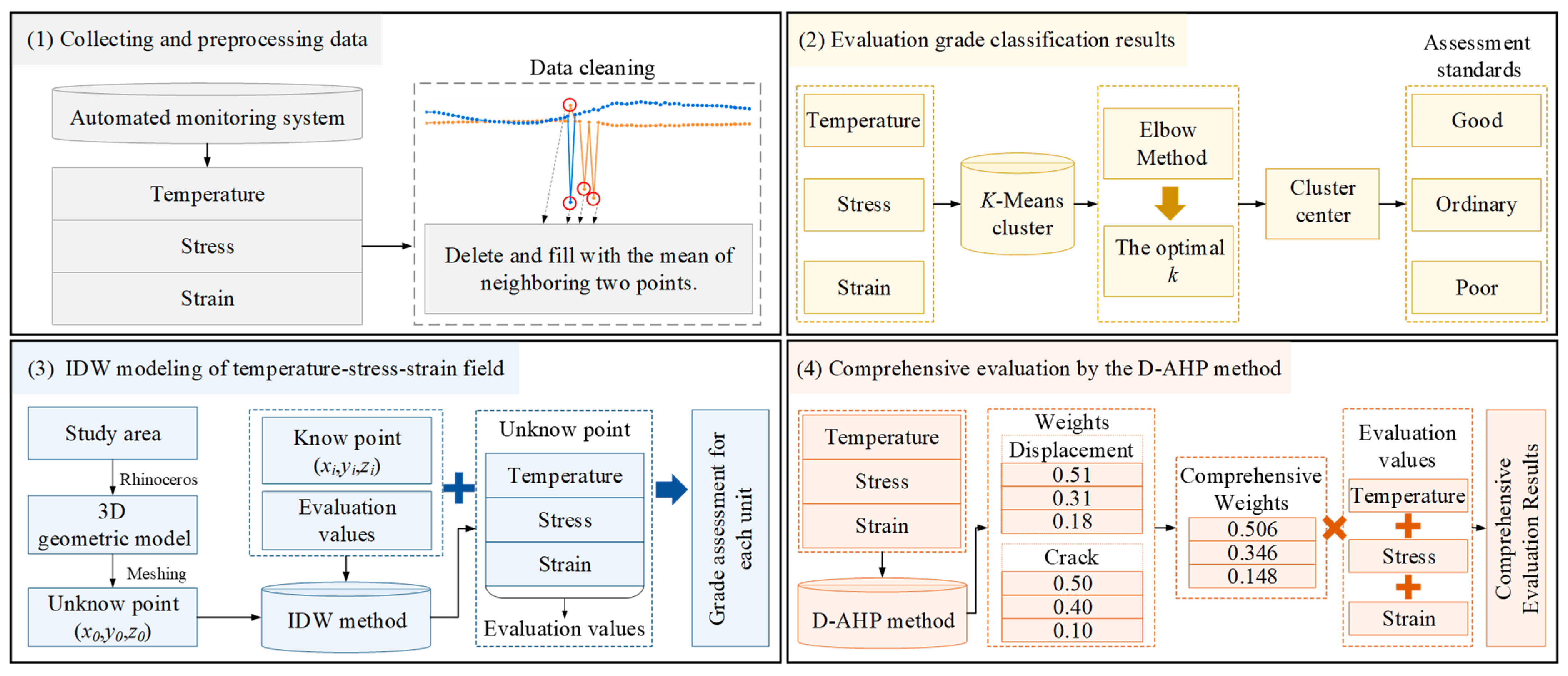
To comprehensively assess the safety status of the dam, this paper adopts the following four modules: (1) collecting and processing long-term monitoring data of dam temperature, stress, and strain, (2) applying the K-means to classify temperature, stress, and strain data to determine grading criteria, (3) conducting a grade assessment of stress, strain, and temperature for each unit using the IDW method, and (4) utilizing the D-AHP method to calculate the weights of each indicator for comprehensive evaluation. Figure 1 illustrates the overall workflow of the methods proposed in this paper.
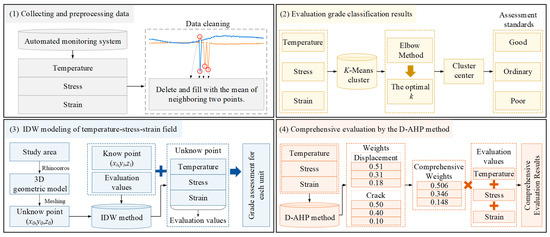
Figure 1.
The overall flowchart.
2.1. K-Means Algorithm
K-means clustering is a widely used unsupervised learning algorithm [19]. It groups data points into several clusters, such that the similarity among data points within the same cluster is high, while the similarity among data points across different clusters is low.
Suppose there are n data points x1, x2, …, xn, and k clusters, where the center of each cluster Si is denoted by ui. The objective of K-means clustering is to minimize the sum of squared distances between data points within a cluster and their cluster center. The objective function can be defined as:
where represents the Euclidean distance from the data point x to its cluster center ui.
The basic steps of the K-means clustering algorithm are as follows:
(1) Randomly select K data points as the initial cluster centers.
(2) For each data point, calculate its distance to all cluster centers and assign it to the cluster represented by the nearest cluster center.
(3) Recalculate the center of each cluster, typically taking the mean of all points in the cluster as the new cluster center.
(4) Repeat the assignment and update steps until the cluster centers no longer change significantly or a predetermined number of iterations is reached.
2.2. Inverse Distance Weight
IDW proposed by Franke [20], is a commonly used spatial interpolation method, widely used in anomaly detection of distributed photovoltaic power stations [21], rainfall, and temperature distributions [22]. The core assumption of the IDW method is that the attribute value of an unsampled point in space is the weighted average of the values of known points around it. This weighted average considers the distances between points; the closer a known point is to the unsampled point, the greater its influence on the attribute value of that point. In this study, the IDW method is employed to calculate the evaluation values for other elements in three-dimensional space. The specific steps are as follows:
(1) Determine the coordinates (x0, y0, z0) of the unsampled point where attribute value prediction is required, and select the surrounding known points and their attribute values.
(2) For each known point (xi, yi, zi), calculate its spatial distance di to the unsampled point and calculate the corresponding weight wi based on this distance. The specific formula is:
where p is the power of the distance. The selection criterion for p is the mean absolute error and the larger p is, the smoother the results are. Here p is set to 2, which is a frequently used value to interpolate precipitation.
(3) Use the weights and the known points’ evaluation values to calculate the predicted evaluation value V0 of the unsampled point, the formula is:
where Vi is the evaluation value of the i-th known point.
2.3. D-AHP Method
The analytic hierarchy process (AHP), first developed by Saaty [23,24], is a structured technique for handling complex decision making by combining qualitative and quantitative analyses. The AHP is used in many fields to make a complex decision due to its ease of use. Burayu [25] applied AHP to identify flood-vulnerable and risk areas. Ahadi [26] proposed an AHP approach to select the optimal site selection for a solar power -plant. In a real situation, an expert may have limited knowledge of and experience with alternatives. As a result, the preferred information may be incomplete and contain fuzziness. The AHP is unable to handle the incomplete information. To solve these problems effectively, a decision-making method using uncertain information called the DAHP method is introduced here. The D numbers were developed by Deng as an effective representation of uncertain information and are widely used in many applications. Deng et al. [27] introduced the D numbers specifically by giving some samples. Fan et al. [28] extended the traditional AHP with the D number to make a hybrid evaluation for curtain grouting efficiency. Zong et al. [29] applied the D numbers to build a more effective model to evaluate university scientific research ability. It shows that the D-AHP is effective in making a comprehensive evaluation.
The D numbers are defined as follows:
Definition 1.
Make be a finite nonempty set, a D number is a mapping formulated by
With
where B is a subset of , is an empty set. It can be seen that the information is completed when , while the information is incomplete when .
The fuzzy preference relation is applied to build comparison matrices based on expert experience. It is described by an additive reciprocal matrix (). rij shows the preference degree of an alternative Ai to the other alternative, Aj, and the preference relation can be expressed as in Equation (7).
However, it is difficult to construct a fuzzy preference relation if the expert assessments are unsure. To solve the problem, Deng et al. [27] used D numbers to develop the classical fuzzy preference relation. At the same time, the D number is defined as in Definition 2:
Definition 2.
The D numbers preference relationship, RD, on a set of alternatives, A, is shown by the D matrix on the set A × A. Its elements are calculated by
The D numbers preference relation is shown in Equation (9).
where , and , , . The preference relations of the different cases are presented in Equations (10) and (11), respectively.
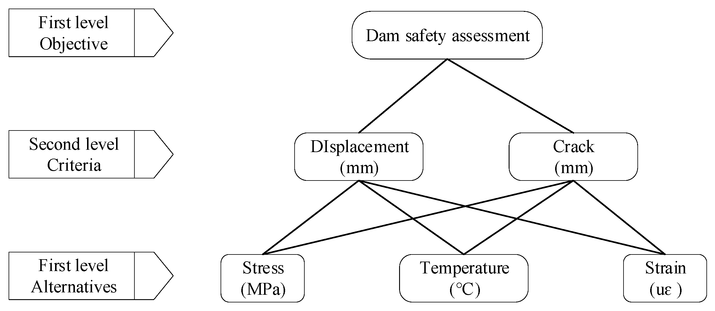
The details of the D-AHP method can be found in Deng et al. [27]. According to the theory, we constructed the D-AHP model for dam safety evaluation, as shown in Figure 2.
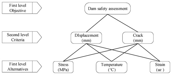
Figure 2.
Hierarchical model for dam safety.
3. Case Study
3.1. The Dam and Monitoring System
As shown in Figure 3, the dam was built on the Yangtze River in China. It is 2595 m long with a maximum depth of 47 m. It contains two power stations (Dajiang and Erjiang stations), with a total electric generating capacity of 2.71 GW. The construction of the dam began in 1970 and was completed in 1988. Some basic information about the Dam is listed in Table 1.
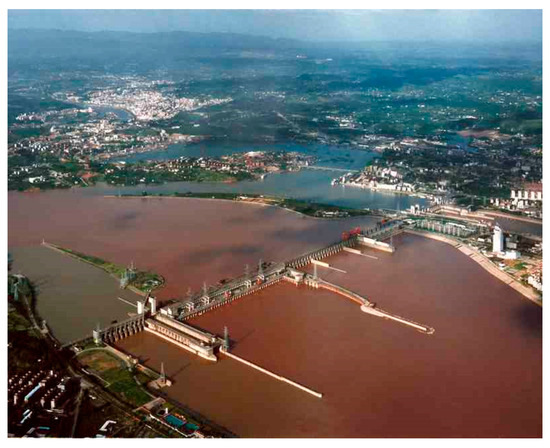
Figure 3.
A general view of dam.

Table 1.
General parameters of the dam.
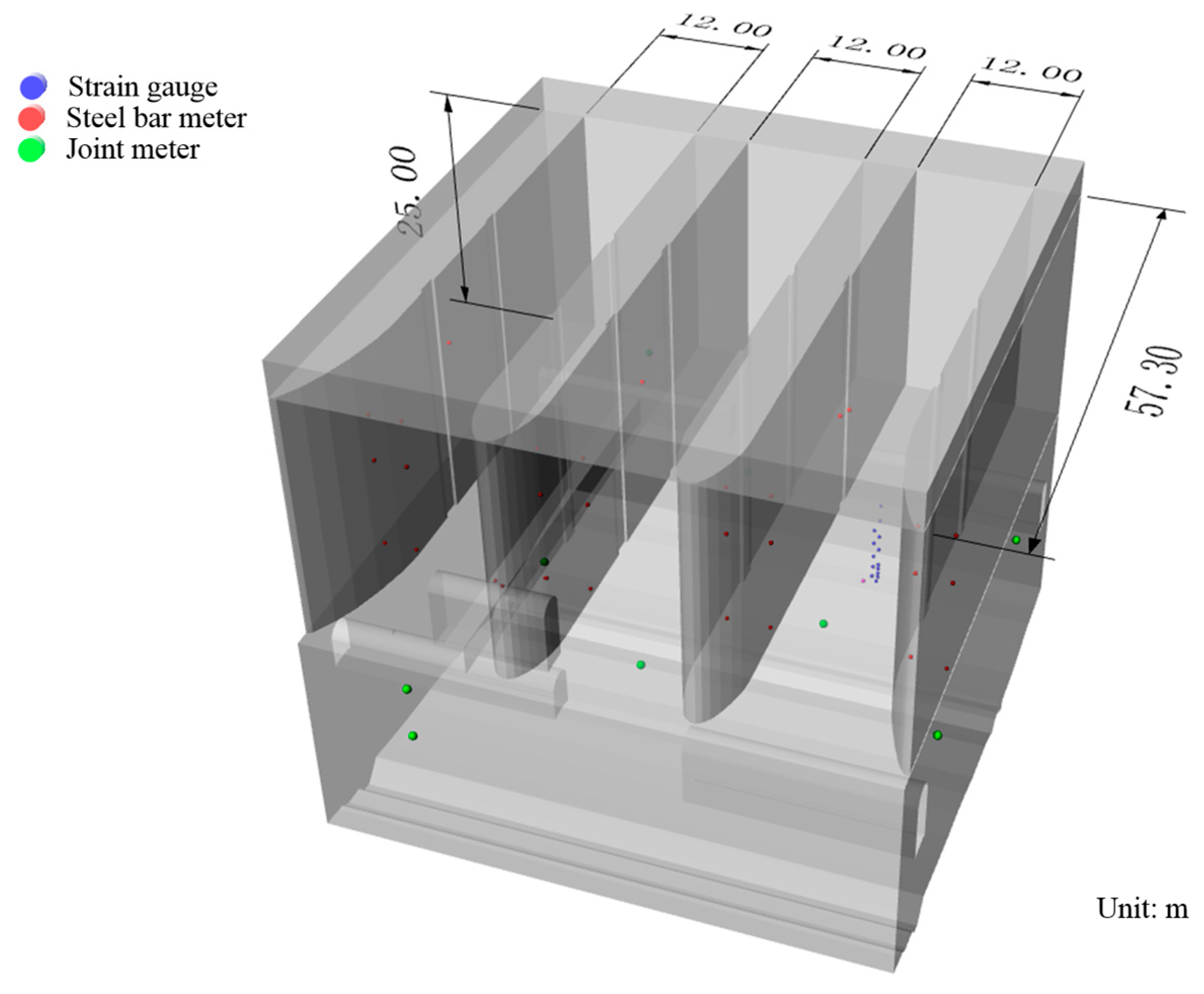
Three sluice openings in the Dajiang scouring sluice were selected for this study. The chamber of the sluice is 57.3 m long, 12.0 m wide, and 25.0 m high. Three types of monitoring recorders, including 21 steel bar meters, 13 strain gauges, and 10 joint meters were used in the dam. Most of them can output temperature except 8 joint meters. However, only 17 steel bar meters and 9 strain gauges can output reliable stress and strain data, respectively. The three types of devices were buried in the dam to be part of the monitoring system permanently. The layout of the monitoring system is shown in Figure 4. The monitoring period was from 1 January 2008 to 30 December 2013. Each set of data was obtained every 5 days. Actually, there were 428 data in each dataset because of some errors in monitoring.
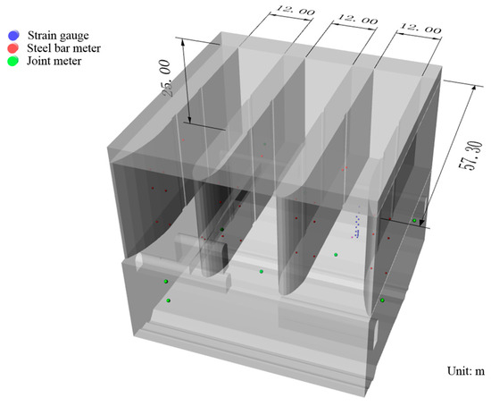
Figure 4.
3D model of the monitoring layout.
3.2. Data Mining by Long-Term Monitoring Records
3.2.1. Data Cleaning
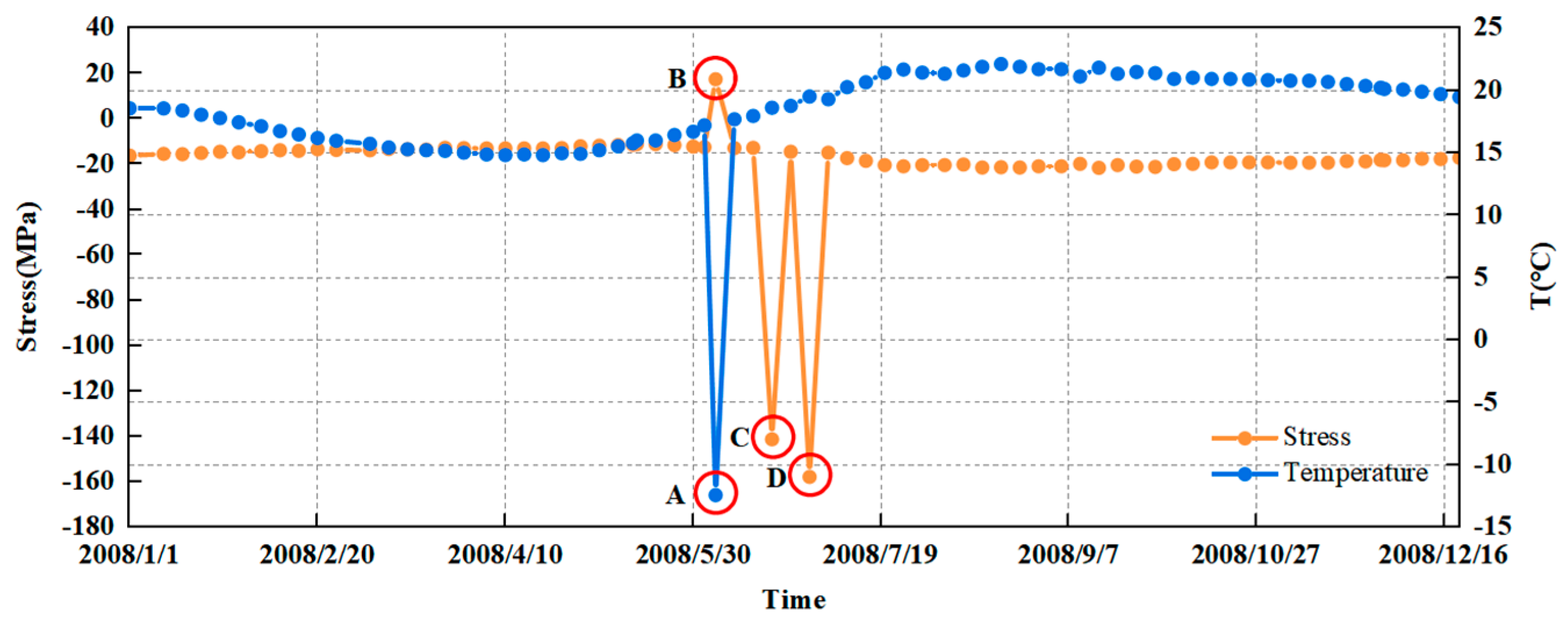
Data cleaning is carried out as a pre-procedure to the data mining. Some monitored data must be filtered out because of instrument failure, as shown in Figure 5.
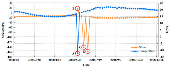
Figure 5.
The diagram of anomalous data.
It is obvious that the four points A, B, C, and D are abnormal. In this study, a method based on data continuity was adopted to identify and eliminate these outliers. Specifically, if the value of a data point differs significantly from its neighboring points, it is considered to be a potential anomaly caused by a temporary malfunction. To rectify this, the average of the values of the two neighboring points on either side of the anomalous data point is calculated, and this average value is used to replace the original outlier. This method not only removes abnormal errors but also maintains the coherence and authenticity of the data.
3.2.2. Evaluation Grade Classification Results
In predicting dam behavior, water level, environment temperature, and time are commonly used as the main predictive indicators. Considering that stress and strain data more directly reflect the dam’s safety condition, this study uses these as the primary analysis indicators. Additionally, considering the significant impact of changes in the dam’s internal temperature on structural safety, the data are also included in the analysis to comprehensively assess the dam’s safety. To more effectively capture the impact of temperature changes when using the K-means clustering algorithm to process data, the temperature data were preprocessed by calculating its mean and standard deviation, and these two statistical measures were used as input parameters for the algorithm.
In K-means clustering, determining the most suitable k value is a crucial step. This study employs the “Elbow Method” to find the optimal k, with the following steps:
(1) For each k from 1 to a certain maximum value, run K-means clustering and calculate the within-cluster sum of squares error for each model, with its formula being:
(2) Plot the errors E for each k on a graph to form a curve.
(3) Observe the curve and identify the point where it starts to bend significantly or flatten. This point is often considered the optimal k value, as improvements from increasing the number of clusters beyond this point are minimal.
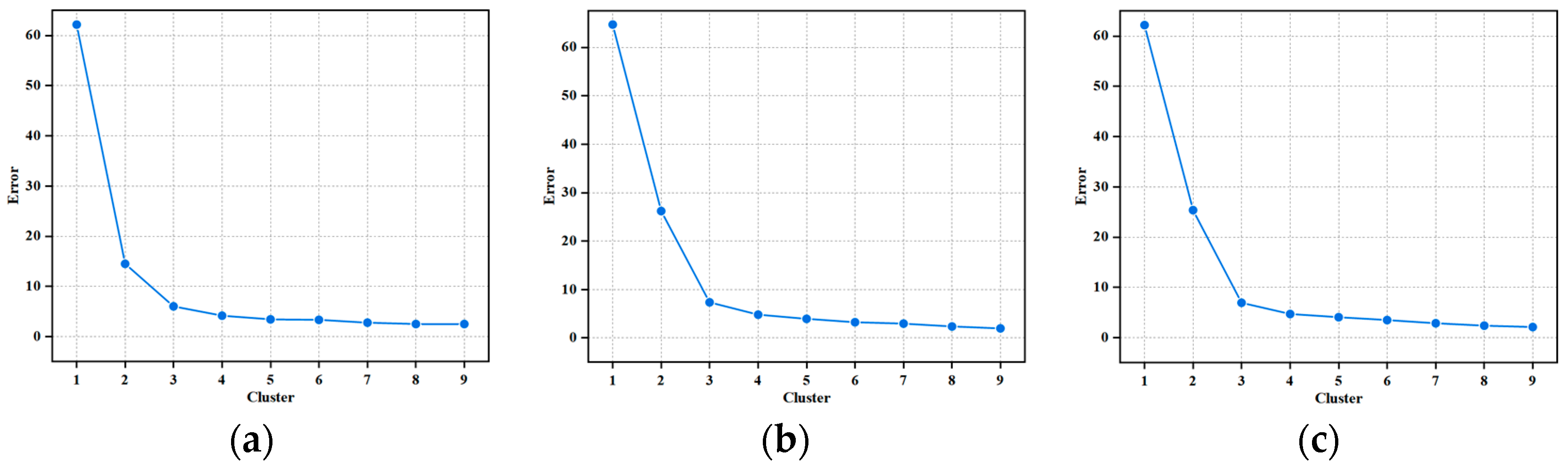
The range of k values is set from 1 to 9. The assessment curve of the clustering effect is plotted according to the steps mentioned above, as shown in Figure 6. From Figure 6, it can be seen that the optimal k value for the datasets of stress, strain, and temperature is 3. Therefore, the safety assessment of the dam is divided into three levels: good, ordinary, and poor, with the corresponding classification standards set as V = {good, ordinary, poor} = {I, II, III}. The values corresponding to the three cluster centers represent the assessment standards for each level, as shown in Table 2.
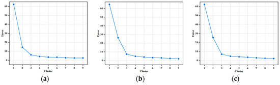
Figure 6.
The evaluation curve of k-value selection. (a) Stress, (b) strain, and (c) temperature.
Table 2.
Assessment standard for the evaluation indicators.
By assigning each data point to the nearest cluster center, each dataset’s measurement points have been explicitly allocated an evaluation value, as detailed in Table 3, Table 4 and Table 5. These evaluation values are denoted as E-values. The assessment values are used to quantify the safety condition of the dam, with numerical values of 1, 2, and 3 assigned to represent the dam’s safety levels, respectively. This method of quantification helps in quickly identifying areas that require attention, allowing for timely maintenance and repair measures.
Table 3.
Stress evaluation.
Table 4.
Strain evaluation.
Table 5.
Temperature evaluation.
3.3. IDW Modeling of Temperature-Stress-Strain Field
The study used Rhinoceros to construct a 3D geometric model and performed a meshing process, which resulted in a mesh model containing a total of 16,921 elements. This meshing process not only provides the geometric shape of the model but also allows for the acquisition of the exact coordinates of all elements. Some elements’ evaluation values and their corresponding coordinates are known, which enables us to apply the IDW method to estimate the evaluation values of the unknown elements.
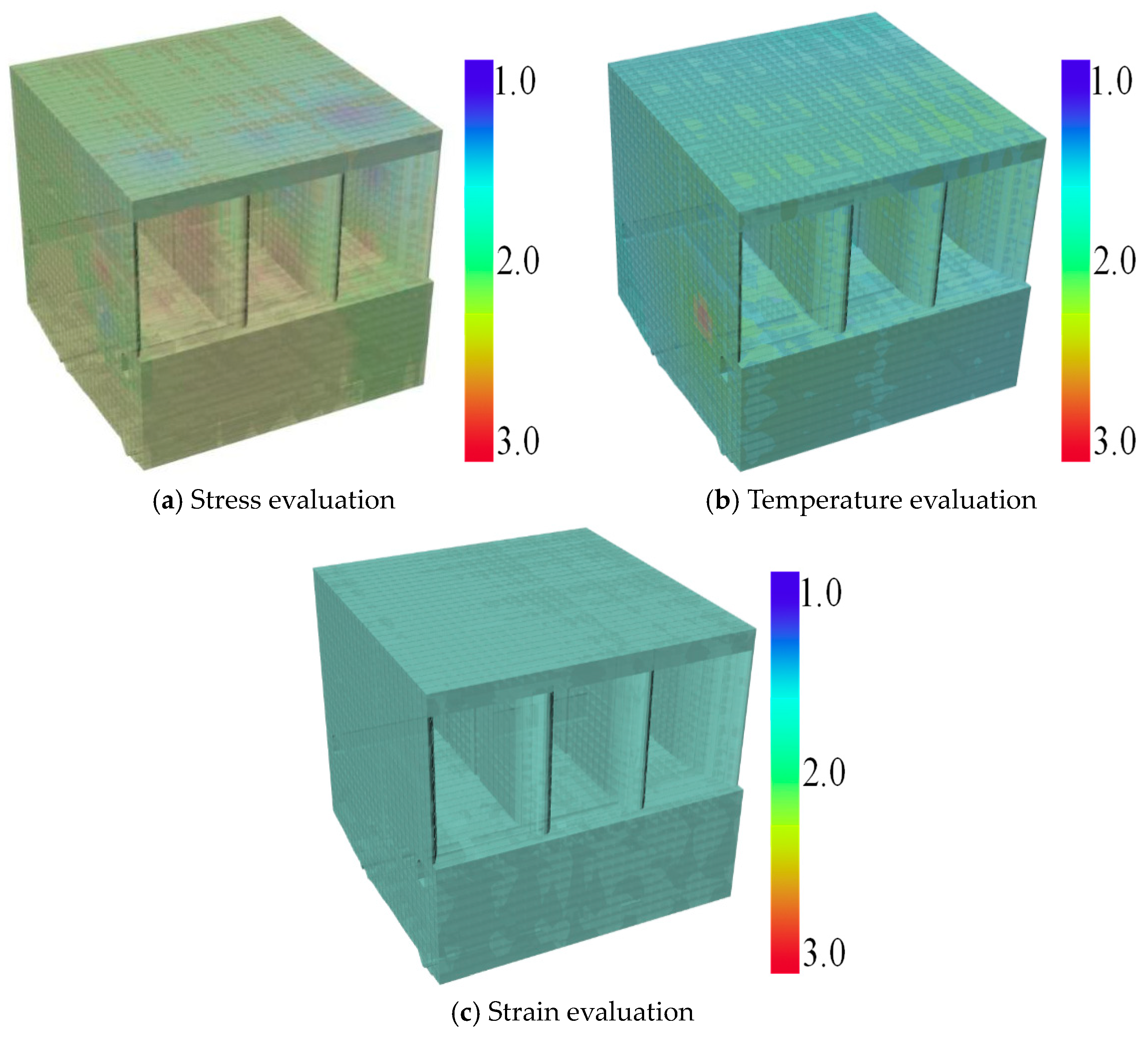
After completing the calculation of the evaluation values for the entire 3D model according to the steps described in Section 2.2, the isoline surfaces can be created to display the variations in evaluation values throughout the space. The range of evaluation values is set between 1 and 3. Three sections are displayed using three different colors. Figure 7 shows examples of three evaluation fields.

Figure 7.
Three evaluation fields.
From Figure 7a, it can be observed that the stress evaluation values vary widely, reflecting the influence of gravity, water pressure, and other factors on the dam. The stress at the bottom of the gates and the piers is greater than at the top, which is consistent with actual conditions. In Figure 7b, the highest temperature value is shown at location R80−3. Figure 7c indicates that, based on the analysis of strain data, the structure of the dam is safe. The above analysis shows that different types of data can reflect different evaluation results, emphasizing the importance of conducting a comprehensive assessment of the study area.
4. Comprehensive Evaluation by the D-AHP Method
After completing the IDW modeling of temperature, stress, and strain fields, this section will employ the D-AHP method introduced in Section 2.3 to conduct a comprehensive analysis of these key factors and calculate their weights in the safety assessment of the dam. Taking the calculation of the weights of these factors on displacement impact as an example demonstrates the application of this method.
4.1. Calculating Weights of Indicators
The D matrix can be established for the weight calculation. We present the procedure of calculating the weights of the indicators with respect to the criteria displacement. First, we calculate the relative significance of stress, temperature, and strain relative to the displacement to build the D matrix based on the D numbers preference relation, as shown in Equation (13).
The RD matrix is converted to a matrix RC as shown in Equation (14):
Then construct a probability matrix RP based on the matrix RC. The probability matrix can be expressed as follows:
The parameters are calculated as: in the triangularization method, where “” means preference.
The triangulated matrix is obtained from matrix RC by the order of I1, I2, and I3. But in this research, equals RC.
Considering the necessary constraints, the weights are calculated in Equation (17):
where wi indicates the weight of indicators. λ is related to the experts’ ability. The λ can be set as in Equation (18).
λ = = 1 was chosen. The weight of I1, I2, and I3 is 0.51, 0.31, and 0.18, respectively. According to the above steps, the weights of temperature, stress, and strain on crack impact can also be calculated. Eventually, the overall evaluation weights can be calculated objectively by calculating the weights in each element. The result is shown in the right column of Table 6. The weights determined through the D-AHP method are not only based on empirical data but also incorporate expert insights and experience, contributing to the formation of a more comprehensive and balanced safety assessment of the dam.
Table 6.
Weights of the indicators.
4.2. Comprehensive Evaluation Results
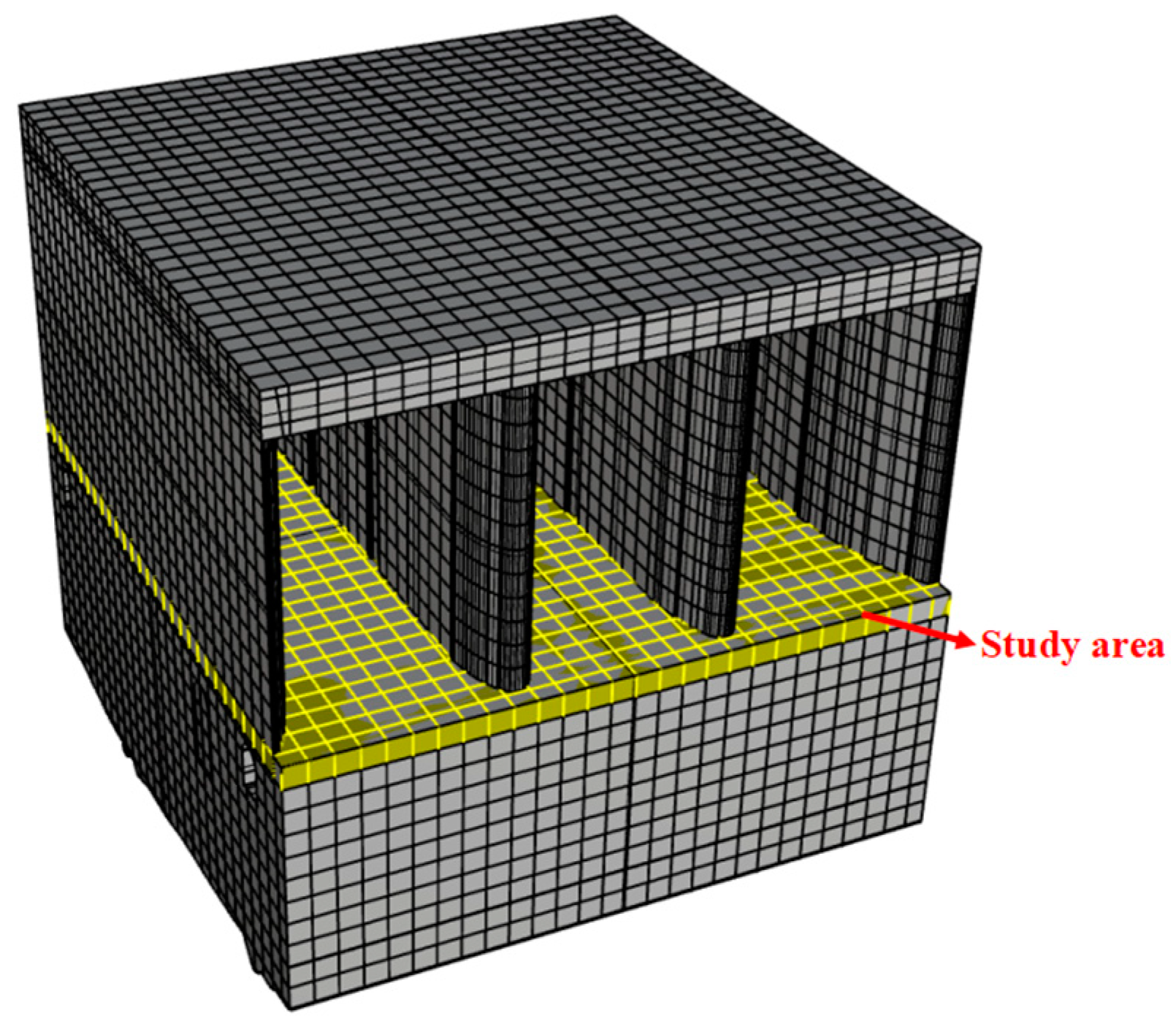
In this section, the bottom plate of the sluice gate is chosen for research analysis, which is prominently highlighted within the entire structure, as shown in Figure 8. Figure 9a illustrates the actual locations of cracks and displacements inside the dam, indicating that they are primarily concentrated in the vicinity of the internal door slots of the dam. Several noticeable cracks were observed at one of the gate slots on the chamber wall (Zone B). These structural issues extend downward along the sluice gate to the bottom, indicating this area as a potential risk point.

Figure 8.
The chosen study region.
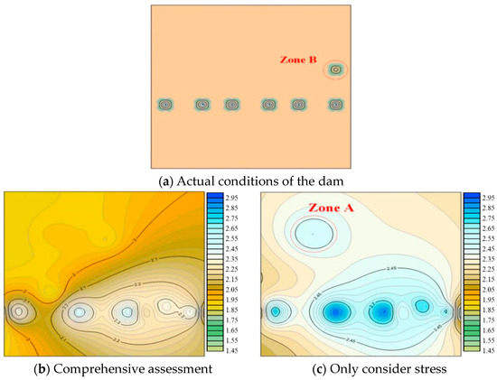
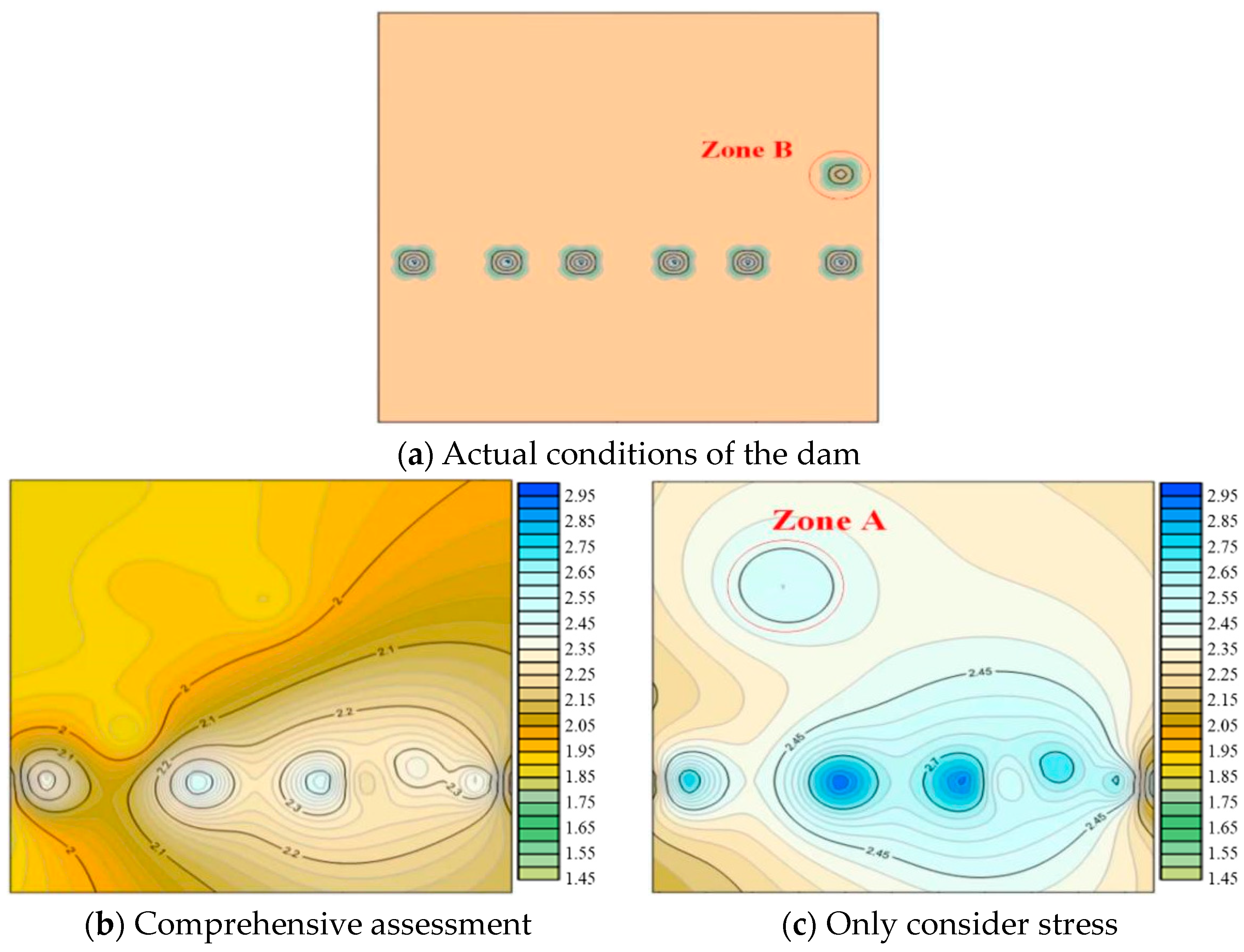
Figure 9.
Comparison of dam safety evaluated by the original and proposed method.
Based on the weights of each indicator obtained from Table 6, we conducted a comprehensive assessment of the selected study area. By weighting the evaluation indicators obtained through the IDW method with their respective weights, we calculated the comprehensive risk assessment values for various parts of the dam. Subsequently, these assessment values were mapped onto a chromatogram to generate contour maps of comprehensive assessment, as shown in Figure 9b. To validate the superiority of our proposed method, we also generated contour maps based on a single stress indicator evaluation for comparison, as shown in Figure 9c.
From Figure 9, it can be seen that both the single stress evaluation method and the comprehensive evaluation method proposed in the study can reveal the development of cracks and displacements near the concrete piers, consistent with the actual situation. However, the single stress assessment method shows a higher risk in region A, but in reality, this location did not experience significant displacements or cracks. The reason for this difference may be the effective measures implemented during construction to prevent cracks and displacements. Therefore, although this area has endured significant stress, the actual extent of cracks and displacements did not reach the predicted severity. This phenomenon indicates that the single stress evaluation method may lead to misjudgments of structural safety due to its failure to consider other influencing factors. In contrast, the comprehensive evaluation method reduces dependence on a single stress factor, thereby reflecting the true state of the structure more comprehensively. The comprehensive method revealed risks in region B that the single method did not identify, aligning with the actual conditions. In conclusion, the introduction of a multifactor comprehensive evaluation method can provide a more comprehensive and accurate risk assessment perspective, which is of great significance for ensuring the longterm safety and stability of concrete structures.
5. Discussion
This study uses spatial interpolation methods to accurately calculate the estimated values for unsampled points, playing a key role in the safety assessment of dams. Compared to other spatial interpolation methods, the IDW method is more flexible and easier to implement, allowing for a quick and effective estimation of attribute values within the influence range based on distance weights.
The D-AHP method was used to allocate weights to various factors in dam safety assessments, significantly enhancing the objectivity and accuracy of the evaluations. Compared to the traditional AHP method, the D-AHP method demonstrates advantages in handling uncertain information. By defining D-numbers, this study was able to more accurately construct comparison matrices and preference relations, thereby making the safety assessment results more aligned with actual conditions.
The method proposed in this study can quickly generate evaluation results, providing an immediate reference for engineering decisions. Although this rapid assessment may not be as accurate as precise analysis, it still offers valuable information for on-site decision-making and emergency response, especially when resources and time are limited. When applying this method to different dam structures and environments, it is necessary to fully consider data quality, method parameters, and specific environmental factors, and adjustments may be needed based on actual conditions.
6. Conclusions
This study proposes a comprehensive assessment model that integrates the K-means clustering algorithm, IDW spatial interpolation technique, and D-AHP decision method. This integrated model can simultaneously consider temperature, stress, and strain, thereby providing a more comprehensive evaluation of the safety condition of dams. The main conclusions drawn from this study are as follows:
(1) This study modeled the temperature-stress-strain field using the IDW method. This approach utilizes data from surrounding known points to assess the safety level of grid cells without direct measurement data, thereby enhancing the continuity of overall evaluation and laying the foundation for subsequent comprehensive assessments.
(2) Using the D-AHP method, this study allocated weights and conducted comprehensive evaluations of the three factors: temperature, stress, and strain. The application of this method has rendered dam safety assessment more objective and scientifically grounded.
(3) The comprehensive evaluation method proposed was applied to practical engineering and compared with an assessment method considering stress alone. The results indicate that compared to the assessment method focusing solely on a single factor, the adoption of the comprehensive evaluation model can more accurately reflect the actual safety condition of dams, providing more comprehensive and reliable safety assessment results for dams.
Future research could incorporate additional monitoring factors such as water pressure and seismic activity. These monitoring data will help identify and analyze potential risk factors and structural changes, thereby enhancing the accuracy and reliability of the evaluation model. Additionally, future research can explore how to effectively integrate these multi-source data and use advanced data fusion techniques to improve the evaluation model.
Author Contributions
Conceptualization, T.Z.; Methodology, T.Z.; Validation, W.Z.; Investigation, X.S.; Data curation, N.M.; Writing—original draft, N.M.; Writing—review & editing, Z.W. and Y.Z.; Visualization, W.Z.; Supervision, X.S. and Y.Z. All authors have read and agreed to the published version of the manuscript.
Funding
This research was funded by the National Key Research and Development Program of China (Grant No. 2022YFC3004403), and Shaanxi Natural Science Basic Research Program (Grant No. 2024JC-YBQN-0473).
Data Availability Statement
The data presented in this study are available on request from the corresponding author. The data are not publicly available due to the confidentiality of the project information.
Conflicts of Interest
The all authors declare that the research was conducted in the absence of any commercial or financial relationships that could be construed as a potential conflict of interest.
References
- Banerjee, A.; Paul, D.K.; Acharyya, A. Optimization and safety evaluation of concrete gravity dam section. KSCE J. Civ. Eng. 2015, 19, 1612–1619. [Google Scholar] [CrossRef]
- Ren, Q.; Li, M.; Li, H.; Shen, Y. A novel deep learning prediction model for concrete dam displacements using interpretable mixed attention mechanism. Adv. Eng. Inform. 2021, 50, 101407. [Google Scholar] [CrossRef]
- Gu, C.; Li, B.; Xu, G.; Yu, H. Back analysis of mechanical parameters of roller compacted concrete dam. Sci. China Technol. Sci. 2010, 53, 848–853. [Google Scholar] [CrossRef]
- Yu, H.; Wu, Z.; Bao, T.; Zhang, L. Multivariate analysis in dam monitoring data with PCA. Sci. China Technol. Sci. 2010, 53, 1088–1097. [Google Scholar] [CrossRef]
- Aly, T.; Sanjayan, J.G.; Collins, F. Effect of polypropylene fibers on shrinkage and cracking of concretes. Mater. Struct. 2008, 41, 1741–1753. [Google Scholar] [CrossRef]
- Castilho, E.; Schclar, N.; Tiago, C.; Farinha, M.L.B. FEA model for the simulation of the hydration process and temperature evolution during the concreting of an arch dam. Eng. Struct. 2018, 174, 165–177. [Google Scholar] [CrossRef]
- Qiang, S.; Xie, Z.; Zhong, R. A p-version embedded model for simulation of concrete temperature fields with cooling pipes. Water Sci. Eng. 2015, 8, 248–256. [Google Scholar] [CrossRef]
- Zhang, L.; Liu, Y.; Li, B.; Zhang, G.; Zhang, S. Study on real-time simulation analysis and inverse analysis system for temperature and stress of concrete dam. Math. Probl. Eng. 2015, 2015, 306165. [Google Scholar] [CrossRef]
- Zhong, R.; Hou, G.; Qiang, S. An improved composite element method for the simulation of temperature field in massive concrete with embedded cooling pipe. Appl. Therm. Eng. 2017, 124, 1409–1417. [Google Scholar] [CrossRef]
- Li, M.; Si, W.; Du, S.; Zhang, M.; Ren, Q.; Shen, Y. Thermal deformation coordination analysis of CC-RCC combined dam structure during construction and operation periods. Eng. Struct. 2020, 213, 110587. [Google Scholar] [CrossRef]
- Zhang, Y.; Zhong, W.; Li, Y.; Wen, L. A deep learning prediction model of DenseNet-LSTM for concrete gravity dam deformation based on feature selection. Eng. Struct. 2023, 295, 116827. [Google Scholar] [CrossRef]
- Rakić, D.; Bojović, M.; Vulovic, S.; Zivkovic, M.; Divac, D.; Milivojević, N. Stability Analysis of Concrete Gravity Dam Using FEM; University of Kragujevac: Kragujevac, Serbia, 2017. [Google Scholar]
- Li, B.; Zhang, Z.; Liu, Y.; Yang, S. Evaluation standard for safety coefficient of roller compacted concrete dam based on finite element method. Math. Probl. Eng. 2014, 2014, 601418. [Google Scholar] [CrossRef]
- Zhang, S.; Zheng, D.; Liu, Y. Deformation prediction system of concrete dam based on IVM-SCSO-RF. Water 2022, 14, 3739. [Google Scholar] [CrossRef]
- Xing, Y.; Chen, Y.; Huang, S.; Wang, P.; Xiang, Y. Research on dam deformation prediction model based on optimized SVM. Processes 2022, 10, 1842. [Google Scholar] [CrossRef]
- Dai, B.; Gu, C.; Zhao, E.; Qin, X. Statistical model optimized random forest regression model for concrete dam deformation mon-itoring. Struct. Control. Health Monit. 2018, 25, e2170. [Google Scholar] [CrossRef]
- Su, H.; Li, X.; Yang, B.; Wen, Z. Wavelet support vector machine-based prediction model of dam deformation. Mech. Syst. Signal Process. 2018, 110, 412–427. [Google Scholar] [CrossRef]
- Kang, F.; Liu, J.; Li, J.; Li, S. Concrete dam deformation prediction model for health monitoring based on extreme learning machine. Struct. Control. Health Monit. 2017, 24, e1997. [Google Scholar] [CrossRef]
- Han, P.; Wang, W.; Shi, Q.; Yue, J. A combined online-learning model with K-means clustering and GRU neural networks for trajectory prediction. Ad Hoc Netw. 2021, 117, 102476. [Google Scholar] [CrossRef]
- Franke, R. Scattered data interpolation: Tests of some methods. Math. Comput. 1982, 38, 181–200. [Google Scholar]
- Shi, Y.; He, W.; Zhao, J.; Hu, A.; Pan, J.; Wang, H.; Zhu, H. Expected output calculation based on inverse distance weighting and its application in anomaly detection of distributed photovoltaic power stations. J. Clean. Prod. 2020, 253, 119965. [Google Scholar] [CrossRef]
- Tan, J.; Xie, X.; Zuo, J.; Xing, X.; Liu, B.; Xia, Q.; Zhang, Y. Coupling random forest and inverse distance weighting to generate climate surfaces of precipitation and temperature with multiple-covariates. J. Hydrol. 2021, 598, 126270. [Google Scholar] [CrossRef]
- Saaty, T.L. A scaling method for priorities in hierarchical structures. J. Math. Psychology. 1977, 15, 234–281. [Google Scholar] [CrossRef]
- Saaty, T.L. How to make a decision: The analytic hierarchy process. Eur. J. Oper. Res. 1990, 48, 9–26. [Google Scholar] [CrossRef]
- Burayu, D.G.; Karuppannan, S.; Shuniye, G. Identifying flood vulnerable and risk areas using the integration of analytical hierarchy process (AHP), GIS, and remote sensing: A case study of southern Oromia region. Urban Clim. 2023, 51, 101640. [Google Scholar] [CrossRef]
- Ahadi, P.; Fakhrabadi, F.; Pourshaghaghy, A.; Kowsary, F. Optimal site selection for a solar power plant in Iran via the Analytic Hierarchy Process (AHP). Renew. Energy 2023, 215, 118944. [Google Scholar] [CrossRef]
- Deng, X.; Hu, Y.; Deng, Y.; Mahadevan, S. Supplier selection using AHP methodology extended by D numbers. Expert Syst. Appl. 2014, 41, 156–167. [Google Scholar] [CrossRef]
- Fan, G.; Zhong, D.; Yan, F.; Yue, P. A hybrid fuzzy evaluation method for curtain grouting efficiency assessment based on an AHP method extended by D numbers. Expert Syst. Appl. 2016, 44, 289–303. [Google Scholar] [CrossRef]
- Zong, F.; Wang, L. Evaluation of university scientific research ability based on the output of sci-tech papers: A D-AHP approach. PLoS ONE 2017, 12, e0171437. [Google Scholar] [CrossRef]

Disclaimer/Publisher’s Note: The statements, opinions and data contained in all publications are solely those of the individual author(s) and contributor(s) and not of MDPI and/or the editor(s). MDPI and/or the editor(s) disclaim responsibility for any injury to people or property resulting from any ideas, methods, instructions or products referred to in the content. |
© 2024 by the authors. Licensee MDPI, Basel, Switzerland. This article is an open access article distributed under the terms and conditions of the Creative Commons Attribution (CC BY) license (https://creativecommons.org/licenses/by/4.0/).