
Study on the Coefficient of Apparent Shear Stress along Lines Dividing a Compound Cross-Section


Abstract
1. Introduction
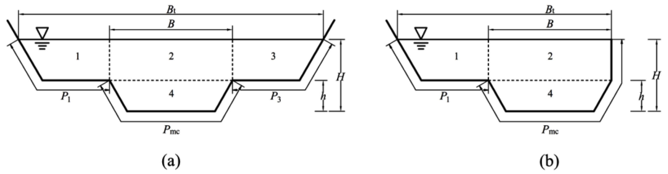
2. Methods
3. Results
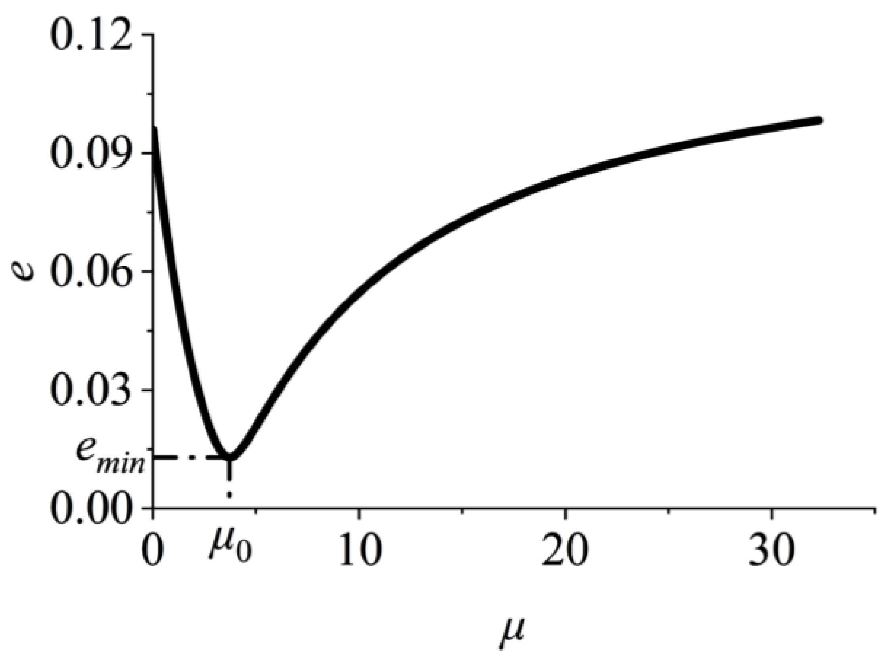
3.1. Existence of μ0
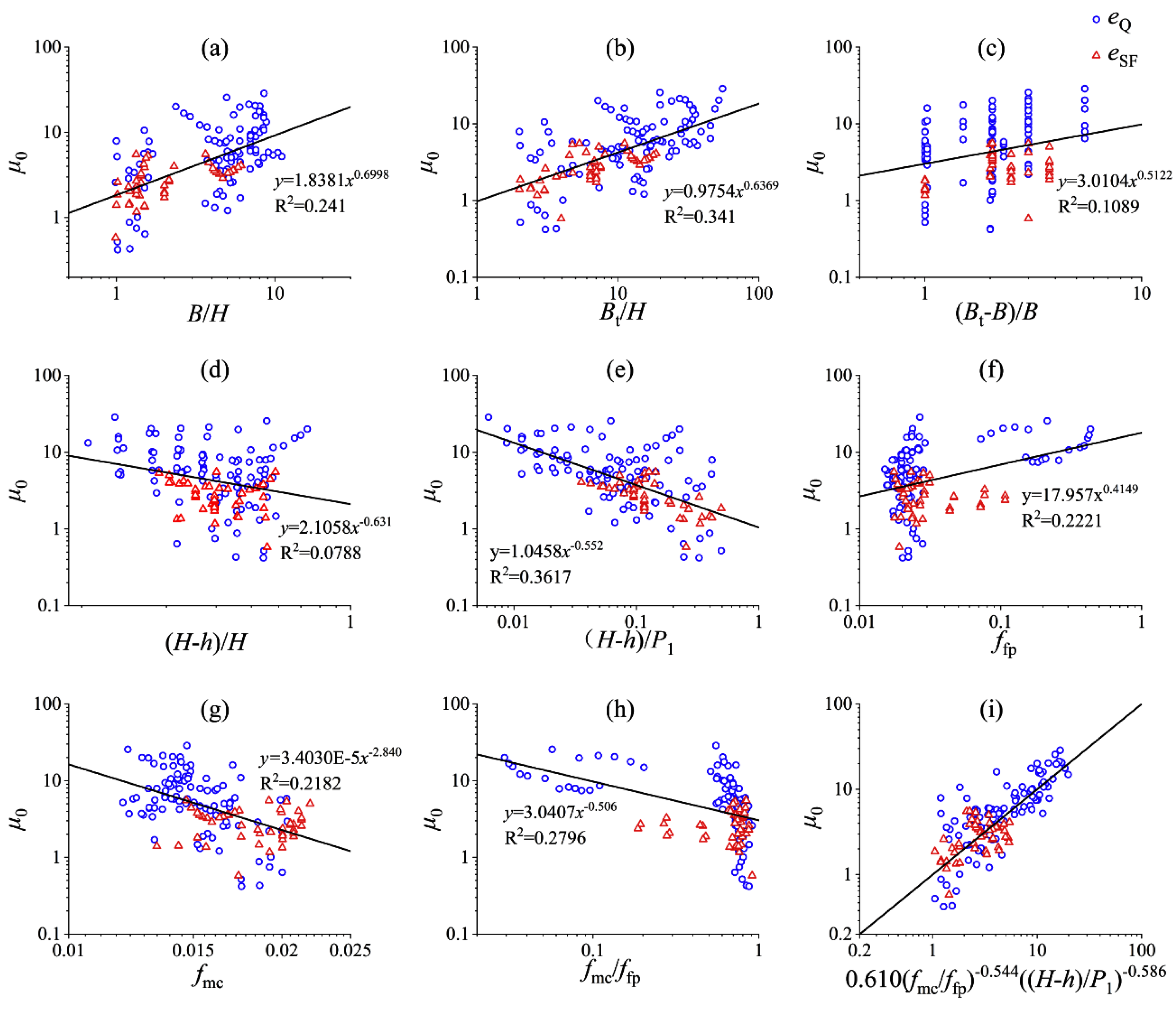
3.2. Influencing Factors and Empirical Formulas
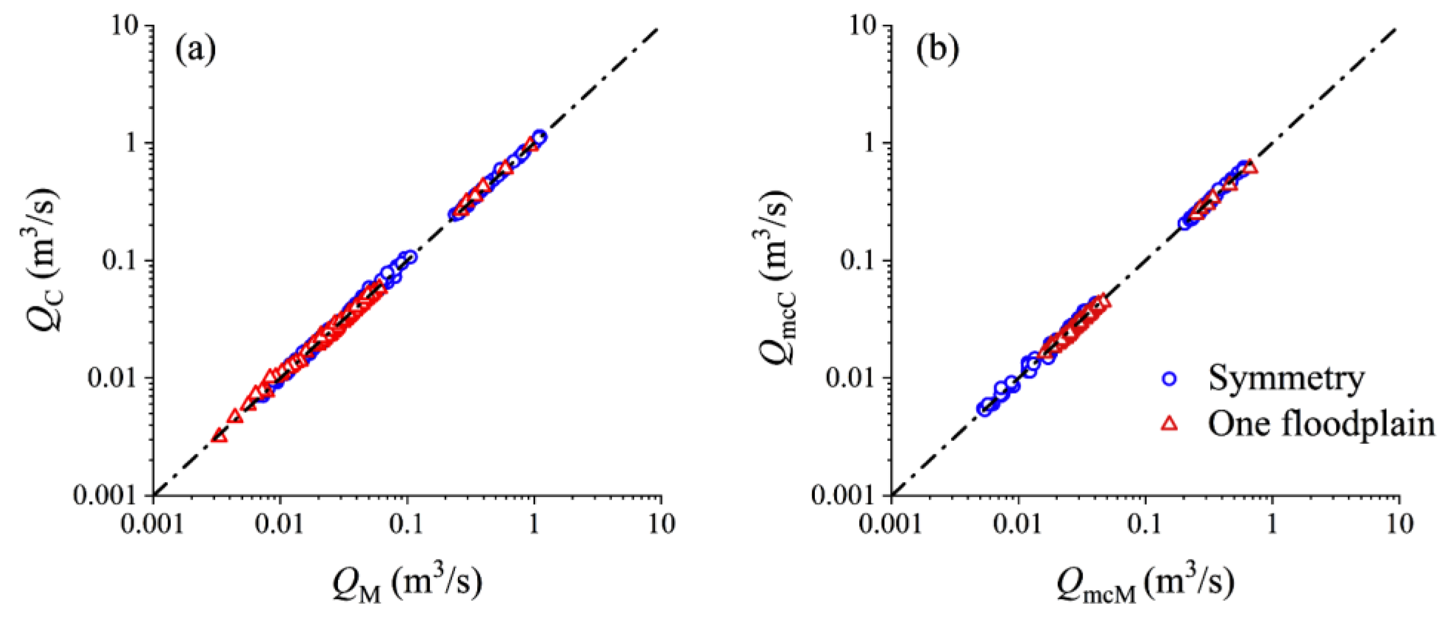
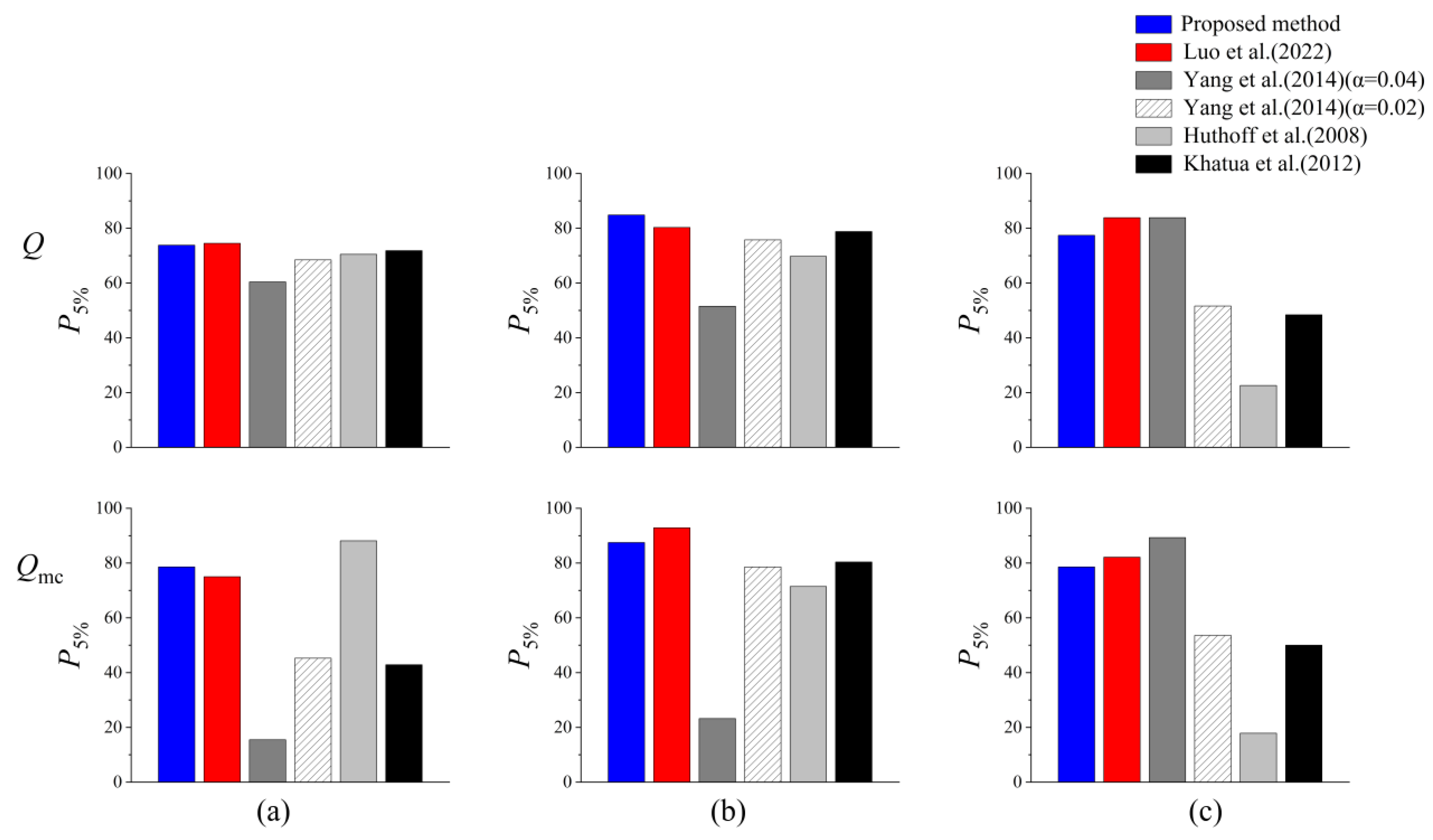
3.3. Comparisons between Different Methods
4. Discussion
4.1. Comparison between Different Empirical Formulas
4.2. Overfitting Problem and the Origin of the Error
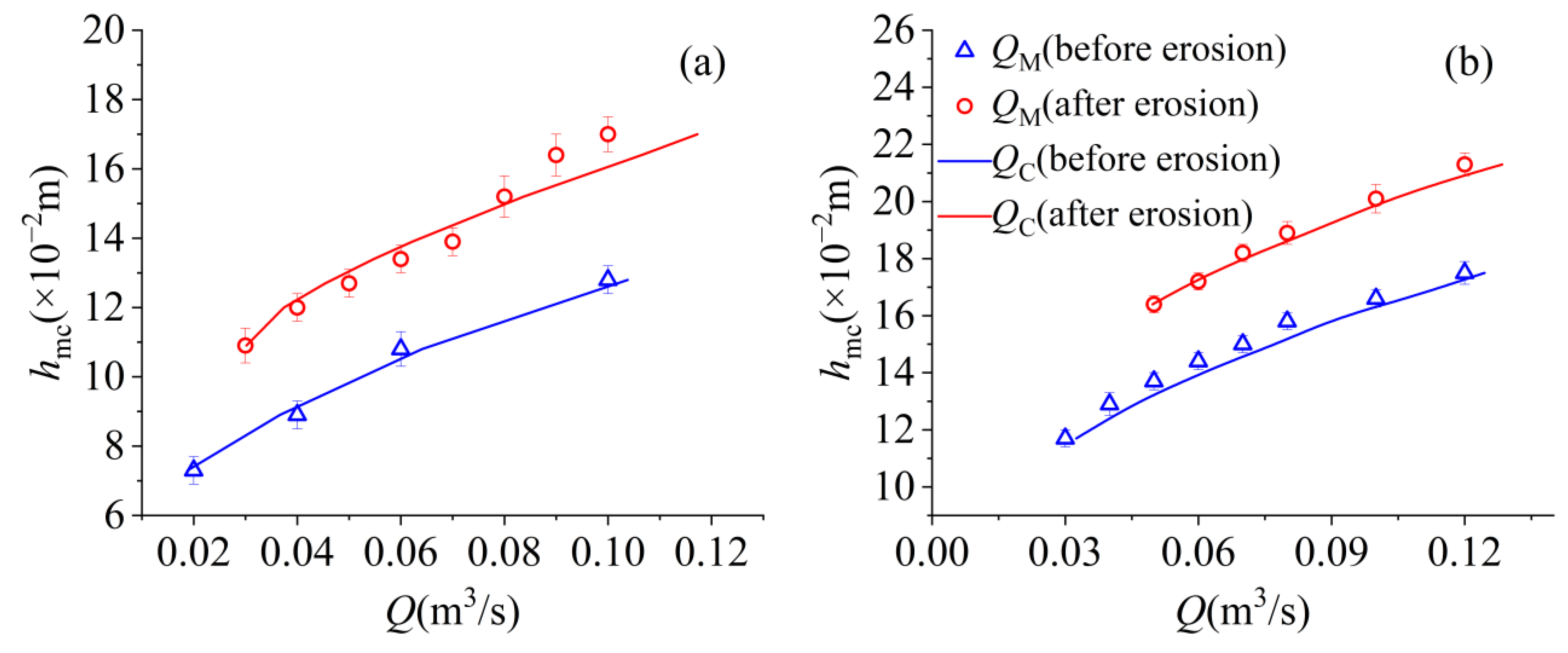
4.3. Erodible Channels
5. Conclusions
Author Contributions
Funding
Data Availability Statement
Acknowledgments
Conflicts of Interest
References
- Ackers, P. Flow formulae for straight two-stage channels. J. Hydraul. Res. 1993, 31, 509–531. [Google Scholar] [CrossRef]
- Myers, W.R.C. Velocity and Discharge in Compound Channels. J. Hydraul. Eng. 1987, 113, 753–766. [Google Scholar] [CrossRef]
- Knight, D.W.; Demetriou, J.D. Flood plain and main channel flow interaction. J. Hydraul. Eng. 1983, 109, 1073–1092. [Google Scholar] [CrossRef]
- Stephenson, D.; Kolovopoulos, P. Effects of momentum transfer in compound channels. J. Hydraul. Eng. 1990, 116, 1512–1522. [Google Scholar] [CrossRef]
- Yen, C.L.; Overton, D.E. Shape effects on resistance in flood-plain channels. J. Hydraul. Div. 1973, 99, 219–238. [Google Scholar] [CrossRef]
- Holden, A. Shear Stresses and Discharges in Compound Channels. Master’s Thesis, University of the Witwatersrand, Johannesburg, South Africa, 1986. [Google Scholar]
- Yang, S.Q.; Han, Y.; Lin, P.; Jiang, C.; Walker, R. Experimental study on the validity of flow region division. J. Hydro-Environ. Res. 2014, 8, 421–427. [Google Scholar] [CrossRef]
- Han, Y.; Yang, S.Q.; Dharmasiri, N.; Sivakumar, M. Experimental study of smooth channel flow division based on velocity distribution. J. Hydraul. Eng. 2015, 141, 06014025. [Google Scholar] [CrossRef]
- Huthoff, F.; Roos, P.C.; Augustijn, D.C.; Hulscher, S.J. Interacting divided channel method for compound channel flow. J. Hydraul. Eng. 2008, 134, 1158–1165. [Google Scholar] [CrossRef]
- Chen, Z.; Chen, Q.; Jiang, L. Determination of apparent shear stress and its application in compound channels. Procedia Eng. 2016, 154, 459–466. [Google Scholar] [CrossRef]
- Khatua, K.K.; Patra, K.C.; Mohanty, P.K. Stage-discharge prediction for straight and smooth compound channels with wide floodplains. J. Hydraul. Eng. 2012, 138, 93–99. [Google Scholar] [CrossRef]
- Khuntia, J.R.; Devi, K.; Khatua, K.K. Boundary shear stress distribution in straight compound channel flow using artificial neuralnetwork. J. Hydraul. Eng. 2018, 23, 04018014. [Google Scholar]
- Yang, K.; Liu, X.; Cao, S.; Huang, E. Stage-discharge prediction in compound channels. J. Hydraul. Eng. 2014, 140, 06014001. [Google Scholar] [CrossRef]
- Luo, Y.; Zhu, S.; Yan, R.; Zhou, J.; Jiang, C. Momentum Transfer–Equivalent States Assumption of the Apparent Shear Stress in Compound Open-Channel Flow. J. Hydraul. Eng. 2022, 148, 06022007. [Google Scholar] [CrossRef]
- Prinos, P.; Townsend, R.D. Comparison of methods for predicting discharge in compound open channels. Adv. Water Resour. 1984, 7, 180–187. [Google Scholar] [CrossRef]
- Yuen, K.W.H. A Study of Boundary Shear Stress, Flow Resistance and Momentum Transfer in Open Channels with Simple and Compound Trapezoidal cross Sections. Ph.D. Dissertation, University of Birmingham, Birmingham, UK, 1989. [Google Scholar]
- Myers, W.R.C.; Brennan, E.K. Flow resistance in compound channels. J. Hydraul. Res. 1990, 28, 141–155. [Google Scholar] [CrossRef]
- Atabay, S. Stage-Discharge, Resistance and Sediment Transport Relationships for Flow in Straight Compound Channels. Ph.D. Dissertation, University of Birmingham, Birmingham, UK, 2001. [Google Scholar]
- Bousmar, D. Flow modeling in compound channels. Momentum transfer between main channel and prismatic or non-prismatic floodplains. Ph.D. Thesis, Catholic University of Louvain, Ottignies-Louvain-la-Neuve, Belgium, 2002. [Google Scholar]
- Macintosh, J.C. Hydraulic Characteristics in Channels of Complex Cross-Section. Ph.D. Thesis, University of Queensland, St Lucia, QLD, Australia, 1990. [Google Scholar]
- Mohanty, P.K.; Khatua, K.K. Estimation of discharge and its distribution in compound channels. J. Hydrodyn. 2014, 26, 144–154. [Google Scholar] [CrossRef]
- Al-Khatib, I.A.; Dweik, A.A.; Gogus, M. Evaluation of separate channel methods for discharge computation in asymmetric compound channels. Flow Meas. Instrum. 2012, 24, 19–25. [Google Scholar] [CrossRef]
- Patra, K.C.; Sahoo, N.; Khatua, K.K. Distribution of boundary shear in compound channel with rough floodplains. In River Basin Management VII; Brebbia, C.A., Ed.; WIT Press: Southampton, UK, 2012; pp. 99–110. [Google Scholar]
- Knight, D.W.; Hamed, M.E. Boundary shear in symmetrical compound channels. J. Hydraul. Eng. 1984, 110, 1412–1430. [Google Scholar] [CrossRef]
- Guo, L.; Su, N.; Zhu, C.; He, Q. How have the river discharges and sediment loads changed in the Changjiang River basin downstream of the Three Gorges Dam? J. Hydrol. 2018, 560, 259–274. [Google Scholar] [CrossRef]
- Fu, H.; Shan, Y.; Yang, K.; Guo, Y.; Liu, C. Stage–discharge relationship in an erodible compound channel with overbank floods. J. Hydrol. 2024, 635, 131181. [Google Scholar] [CrossRef]

| Sources | Cross-Section Shape | Q (m3/s) | μ0 | α | Amount of Data |
|---|---|---|---|---|---|
| Sub-region discharges (Q) | |||||
| K&D | S | 0.0067~0.029 | 0.42~5.85 | 0.0018~0.0298 | 14 |
| Yuen | S | 0.013~0.055 | 3.39~10.55 | 0.0111~0.0368 | 12 |
| FCF | S/O | 0.24~1.11 | 3.7~28.66 | 0.0112~0.1053 | 43 |
| Atabay | S/O | 0.018~0.08 | 1.25~20.01 | 0.0047~0.0636 | 34 |
| Boundary shear force (SF) | |||||
| K&D | S | 0.0067~0.029 | 0.58~5.52 | 0.0025~0.0265 | 14 |
| Yuen (Yuen 1) | S | 0.013~0.035 | 1.37~1.81 | 0.0046~0.0069 | 4 |
| P&T | S | 0.012~0.026 | 1.72~5.01 | 0.0086~0.2746 | 16 |
| Atabay (ROS-S) | S | 0.018~0.08 | 2.91~5.54 | 0.0115~0.0204 | 13 |
| Sources | H (m) | Bt (m) | Q (m3/s) | μ0 | α | Amount of Data |
|---|---|---|---|---|---|---|
| Experimental data for Symmetric-floodplain | ||||||
| K&D | 0.1~0.15 | 0.3~0.61 | 0.0067~0.029 | 1.05~3.22 | 0.0045~0.016 | 14 |
| Yuen | 0.1~0.15 | 0.45 | 0.013~0.055 | 1.19~2.54 | 0.0035~0.0094 | 12 |
| FCF (S01~S03, S07, S08, S10) | 0.17~0.30 | 3.3~10 | 0.24~1.11 | 2.08~19.81 | 0.0063~0.073 | 37 |
| P&T | 0.13~0.15 | 1.07~1.17 | 0.012~0.026 | 2.48~5.37 | 0.012~0.027 | 16 |
| Atabay (ROS ORH) | 0.07~0.17 | 1.21 | 0.018~0.08 | 2.63~13.06 | 0.01~0.053 | 34 |
| M&K | 0.07~0.12 | 3.95 | 0.015~0.11 | 5.61~20.52 | 0.024~0.105 | 6 |
| Khatua | 0.14~0.22 | 0.44 | 0.0087~0.039 | 1.09~3.03 | 0.0061~0.018 | 10 |
| Patra | 0.11~0.14 | 1.89 | 0.048~0.096 | 3.36~5.51 | 0.014~0.025 | 13 |
| Experimental data for One-floodplain | ||||||
| FCF(S6) | 0.18~0.30 | 6.3 | 0.26~0.93 | 3.46~11.52 | 0.011~0.043 | 6 |
| Atabay (ROA) | 0.07~0.11 | 1.213 | 0.018~0.055 | 2.28~4.97 | 0.0083~0.025 | 22 |
| Bousmar | 0.05~0.08 | 0.8 | 0.0078~0.016 | 3.42~13.08 | 0.02~0.084 | 4 |
| Macintosh | 0.07~0.11 | 1.51~1.62 | 0.019~0.06 | 2.37~14.24 | 0.0086~0.062 | 60 |
| Khatib | 0.05~0.11 | 0.3 | 0.0033~0.014 | 1.15~2.10 | 0.014~0.03 | 12 |
| Method | Khatua | Huthoff | Yang α = 0.04 | Yang α = 0.02 | Luo | Proposed Method | |
|---|---|---|---|---|---|---|---|
| Parameter | |||||||
| P3%(Q) | 56.50 | 41.87 | 41.46 | 46.34 | 53.66 | 54.88 | |
| P5%(Q) | 70.73 | 64.23 | 60.98 | 68.29 | 77.23 | 77.24 | |
| P10%(Q) | 89.84 | 87.80 | 96.74 | 93.90 | 98.78 | 97.15 | |
| NRMSE(Q) × 100 | 1.6 | 1.4 | 0.93 | 1 | 0.51 | 0.59 | |
| P3%(Qmc) | 37.5 | 48.81 | 18.45 | 33.93 | 48.48 | 51.79 | |
| P5%(Qmc) | 56.55 | 70.83 | 30.36 | 57.74 | 82.14 | 81.55 | |
| P10%(Qmc) | 85.71 | 86.90 | 75.00 | 88.69 | 98.80 | 96.43 | |
| NRMSE(Qmc) × 100 | 3.3 | 2.4 | 2.4 | 2 | 0.99 | 0.96 | |
| P0.01(SFmc) | 23.13 | 23.88 | 11.94 | 21.64 | 31.34 | 23.88 | |
| P0.03(SFmc) | 56.72 | 43.28 | 38.06 | 55.22 | 66.42 | 61.94 | |
| P0.05(SFmc) | 73.88 | 76.12 | 73.13 | 82.09 | 86.57 | 82.84 | |
| Formulas | Equation (16) | Equation (20) | Equation (21) | Equation (22) | |
|---|---|---|---|---|---|
| Parameters | |||||
| P3%(Q) | 54.88 | 52.03 | 54.07 | 55.28 | |
| P5%(Q) | 77.24 | 76.83 | 78.86 | 78.45 | |
| P10%(Q) | 97.15 | 95.53 | 97.15 | 96.34 | |
| NRMSE(Q) × 100 | 0.59 | 0.44 | 0.44 | 0.46 | |
| P3%(Qmc) | 51.79 | 42.86 | 42.26 | 47.02 | |
| P5%(Qmc) | 81.55 | 69.64 | 77.38 | 77.38 | |
| P10%(Qmc) | 96.43 | 94.64 | 98.21 | 95.25 | |
| NRMSE(Qmc) × 100 | 0.96 | 1.14 | 1.06 | 1.08 | |
Disclaimer/Publisher’s Note: The statements, opinions and data contained in all publications are solely those of the individual author(s) and contributor(s) and not of MDPI and/or the editor(s). MDPI and/or the editor(s) disclaim responsibility for any injury to people or property resulting from any ideas, methods, instructions or products referred to in the content. |
© 2024 by the authors. Licensee MDPI, Basel, Switzerland. This article is an open access article distributed under the terms and conditions of the Creative Commons Attribution (CC BY) license (https://creativecommons.org/licenses/by/4.0/).
Share and Cite
Zhao, Y.; Chen, D.; Qin, J.; Wang, L.; Luo, Y. Study on the Coefficient of Apparent Shear Stress along Lines Dividing a Compound Cross-Section. Water 2024, 16, 1648. https://doi.org/10.3390/w16121648
Zhao Y, Chen D, Qin J, Wang L, Luo Y. Study on the Coefficient of Apparent Shear Stress along Lines Dividing a Compound Cross-Section. Water. 2024; 16(12):1648. https://doi.org/10.3390/w16121648
Chicago/Turabian StyleZhao, Yindi, Dong Chen, Jinghong Qin, Lei Wang, and You Luo. 2024. "Study on the Coefficient of Apparent Shear Stress along Lines Dividing a Compound Cross-Section" Water 16, no. 12: 1648. https://doi.org/10.3390/w16121648
APA StyleZhao, Y., Chen, D., Qin, J., Wang, L., & Luo, Y. (2024). Study on the Coefficient of Apparent Shear Stress along Lines Dividing a Compound Cross-Section. Water, 16(12), 1648. https://doi.org/10.3390/w16121648