Overflow Simulation and Optimization of a Drainage System in an Urban Area in the Northern Anhui Plain

Abstract

Quantitative simulation of urban waterlogging using computer models is an effective technical means for urban storm water management, especially for predicting and preventing waterlogging. In this study, a city in the northern Anhui Plain, China, was selected as the study site. The Storm Water Management Model was applied to simulate the dynamic changes in the pipeline overload, node overflow, and discharge port runoff characteristics from three perspectives: surface runoff, pipe network transmission, and flow control of low-impact development. The operation of the rainwater pipe network under different return periods and the real-time operation of the rainwater pipe network were simulated to seek solutions to urban waterlogging problems caused by flat terrain and slow drainage. The results revealed that surface runoff is the primary source of rainfall in the study area, with a runoff coefficient of 0.599. The drainage pipe network was optimized by expanding the diameter of the pipe from ≤1.5 mm to ≥2 mm. The water reduction rate was more than 50%, and overload did not occur after optimization. Therefore, sinking green space technology and optimization methods for expanding a pipe diameter can reduce urban waterlogging.

1. Introduction

Rapid urbanization has several consequences; for example, the expansion of ground surface hardening [1] has led to a significant increase in urban surface runoff, which the insufficient capacity of urban drainage systems cannot contain [2], causing frequent urban flooding [3] and serious harm to the lives and properties of residents [4]. Several occasions of urban floodings prove this point. On 1 September 2021 local time, during the onslaught of Hurricane Ida, more than 80 mL of rain poured in just 1 h; consequently, Newark Liberty International Airport was flooded, and an economic loss of USD 50 billion was incurred. Meanwhile, Henan Province in China suffered a rare heavy rainstorm and serious flood disaster on 17–23 July 2021; a total of 14,786,000 people were affected, and the direct economic loss amounted to CNY 120.6 billion [5]. Therefore, to address urban flooding [6], urban drainage systems should be urgently renovated and optimized [7].

In order to prevent the aggravation of urban waterlogging, rainwater pipe networks have been renovated. However, renovation is expensive and the results are not satisfactory. Therefore, many storm water model simulations have been developed at home and abroad, such as the Storm Water Management Model (SWMM) [8], STORM [9], Hydrological Simulation Program-FORTRAN [10], and Info Works ICM [11], have been developed globally to optimize the design of drainage networks. The SWMM was developed by the U.S. Environmental Protection Agency and is mainly used to simulate the complete operational process of sites during an entire rainfall event in a city [8]. It is not limited by the area of the study area or the number of node pipe sections and sub-catchment areas. It has the advantages of easy access to parameters, simple use, and a simple and friendly interface. At the same time, the SWMM5.1 is a non-commercial software, which is both practical and flexible. It has the characteristics of easy access to parameters and high simulation and is most widely used.

The northern plain region of Anhui Province, China, is characterized by gentle topography and poor surface runoff mobility [12]. Additionally, its pipeline is severely silted, broken, and aged, and its drainage capacity has become insufficient [13], which triggers and aggravates the accumulation of surface water [8]. Whenever there is a rainstorm, the low slope of the ground will cause the rapid convergence of water and cause floods. Although many studies have used the SWMM to solve the problem of urban waterlogging, few studies have focused on more serious problems in flat areas. Therefore, it is necessary to use the SWMM to analyze the operating conditions of a drainage pipe network under different rainfall conditions, predict the probability and risk of waterlogging, and evaluate the simulation and optimization of drainage pipe networks for flood control and drainage [14].

The aim of this was to construct and optimize an urban drainage network model [15] using the SWMM [16] combined with ArcGIS for an urban area in northern Anhui Plain. Based on the SWMM, a study area model was constructed, and the urban rainfall scenarios under different return periods were simulated. The improvement methods of expanding a pipe diameter and sinking green space measures are proposed. This study contributes to the alleviation of flooding in the study area and to other urban areas that would apply the methods and models we used.

2. Study Area and Methods

2.1. Overview of the Study Area

Anhui Province is an important transport hub region in central China. The study area is located in Guoyang County, northern Anhui Province. It is between 33°27′ and 33°47′ north latitude and 115°53′ to 116°33′ east longitude, with a total area of 2110 km² (Figure 1). All the rivers that traverse the study area belong to the Huai River system; the main river in the territory is the first-class Guo River, which crosses the central part of the Huai River. The watershed terrain slopes slowly from northwest to southeast. The ground elevation is 30 m, and the average slope is 1 in 10,000. Green space, residential land, industrial land, commercial land, and water area are accounted for, respectively, as 29%, 31%, 24%, 6%, and 4% of total land; other land accounts for 6%. The rivers in the study area all belong to the Huai River water system, and the main rivers in the territory are the first-class tributary of the Huai River, the Guo River, which traverses the central part of the river, and the tributaries on both sides of the vortex river are distributed in the form of leaf veins. The study area is located on the south side of the vortex river, and there are 12 rivers in the area. These rivers are intertwined into a vast network of rivers. The region has a warm, temperate, semi-humid, monsoon climate, with moderate rainfall and a decreasing distribution from southeast to northwest. In the past ten years, there were 646 rainy days. The annual average rainfall is approximately 851.6 mm; approximately 54% of the annual precipitation is concentrated from June to August, especially in July, when strong winds and heavy rain usually occur. There are three soil types in the area: lime concretion black soil, chao soil, and limestone soil. Among them, lime concretion black soil is the largest and most widely distributed soil type in Guoyang County. The water holding capacity of lime concretion black soil is poor, and the effective moisture content is low.

Recently, several serious waterlogging disasters have occurred in the study area and its vicinity. For instance, heavy rainfall in the Anhui region on 4–5 July 2018 led to severe flooding in some areas, affecting 159,300 residents and incurring CNY 80.63 million in economic losses.

2.2. Data Collection

The basic data and information required for the establishment of the model can be divided into two parts: the first set of data included topography, land use type data [17], and pipe network information, while the other set included rainfall data and model operational parameters required for the model’s operation [18].

2.2.1. Rainfall Data

Four rainfall events in 2022 were used as the basic data. The rainfall characteristics and sequences of the four rainfall events are presented in

Table 1. Actual rainfall data in the study area.

Rainfall Time	Rainfall (mm)	Maximum Rainfall Intensity (mm/h)	Average Rainfall Intensity (mm/h)	Rainfall Type
13 June 2022	18.2	5.9	1.82	Moderate rain
23 June 2022	31.6	16.8	3.16	Heavy rain
20 July 2022	63.2	32.7	5.74	Rainstorm
27 August 2022	7.3	2.7	0.52	Light rain

.

To simulate different rainfall intensities, the Chicago Rain Pattern Generator was used to generate the rainfall data; the rainstorm intensity formula used is shown in Equation (1).

$$q=\frac{1321.161\left(1+0.739\lg P\right)}{{\left(t+5.989\right)}^{0.596}}$$

(1)

where q is the rainstorm intensity (L/s∙ha), P is the return period (years), and t is the rainfall duration (min).

Taking the peak ratio as r = 0.4, we input the above storm intensity formula into the Chicago Rain Pattern Generator to obtain the rainfall data within a rainfall duration of 120 min (Figure 2).

The total and average rainfall intensities for each return period are listed in

Table 2. Summary table of design storms by recurrence period.

Recurrence Period/a	120 min Total Cumulative Rainfall (mm)	120 min Average Rainfall Intensity (mm/min)
P = 0.5	41.6299	0.344
P = 1	53.5406	0.4425
P = 2	65.4513	0.5409
P = 5	81.1965	0.671
P = 10	93.1072	0.7695
P = 20	105.0179	0.8679

.

2.2.2. Drainage Network Data

The model was built using rainwater pipe network data as the basic data. To meet the requirements of model establishment, the pipe network data were generalized prior to modelling.

After checking the computer-aided design (CAD) map of the drainage pipe network and importing it into a geographic information system (GIS), which was used to extract and calculate drainage pipe network data, the elevation of each node and the diameter and length of each pipe section were improved, and the topological relationship between the inspection well and pipe section was corrected. The elevation data and pipeline data required for modeling in CAD were retained. After the pipeline data in CAD were divided into different layers according to the pipeline diameter, the pipeline network was generalized by GIS reading and calculation. After importing the rainwater pipeline processed in CAD into the new Feature Dataset in ArcMap, a new Geometric Network was built here, and the required tolerances were input to generate nodes. Finally, a new topological relationship was created in the Feature Dataset, and the node and pipe segment data were verified and corrected. The generalized CAD diagram, the distribution of nodes and pipelines, and the Digital Elevation Model (DEM) data are shown in Figure 3. The revised study area had 224 pipe sections and 343 nodes.

2.2.3. Sub-Catchment Data

The study area was divided into several sub-catchments, and the catchment process was simulated according to the parameters of each sub-catchment. Since the study area was vast and the land use of the subsurface was complicated, digital elevation information, planning maps, and drainage network maps were used. Then, the hydrological analysis module in GIS [19] was applied to divide the study area into sub-catchment areas [20]. The study area was further divided into 87 sub-catchment areas based on actual visits and ocular inspections. The results of the division are shown in Figure 4.

2.3. Model Construction

The extracted drainage pipe network and sub-catchment data were imported into the model, and the initial values of the parameters were selected for model construction. Sensitivity analysis and parameter calibration of the eight parameters in the model were conducted using the modified Morris screening method [21] and runoff coefficient method.

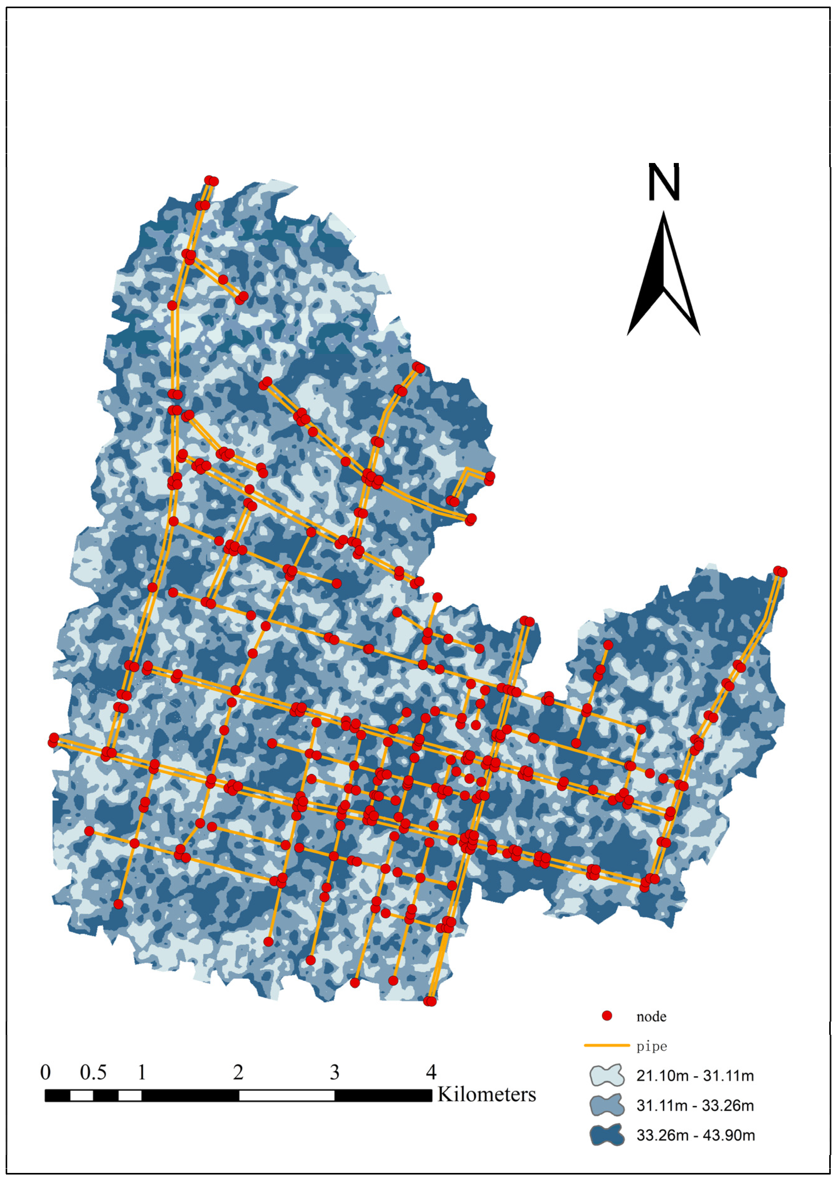
2.3.1. Hydrological and Hydraulic Model Parameter Setting

Hydrological and hydraulic parameters were used for the sub-catchment and drainage pipe network simulations, respectively. The preliminary values of the parameters [22] were analyzed as follows.

(1)

Manning Coefficient

The preliminary Manning coefficient values for different surfaces and pipeline types are listed in

Table 3. Manning coefficient parameters.

	Manning Coefficient
Manning coefficient of permeable zone	Manning coefficient of impermeable zone	Manning coefficient of pipes
0.24	0.012	0.013

.

(2)

Parameters of Infiltration Model

The Horton model is the most widely used and effective infiltration model for constructing a surface runoff model; the preliminary values of its parameters are listed in

Table 4. Horton infiltration model parameters.

Parameter	Value Range	Preliminary Value
Maximum infiltration rate (mm/h)	20–120	79
Minimum infiltration rate (mm/h)	0–20	2.5
Attenuation factor (h−1)	1–7	2
Drainage time (d)	2–14	6

.

(3)

Depression Storage Capacity

Depression storage is classified into two types: permeable and impermeable. It was preliminarily determined that the permeable area depression storage was 6 mm, while the impervious area depression storage was 2.5 mm.

(4)

Comprehensive Runoff Coefficient

By analyzing the space and area of green spaces, roofs, and roads, and weighing the results, the comprehensive runoff coefficient of the study area was determined to be 0.599 (

Table 5. Integrated runoff coefficient calculation.

Lower Cushion Surface	Area/km2	Total Area/km2	Proportion of Total Area	Runoff Coefficient	Comprehensive Runoff Coefficient
Greenbelt	17.56	46.69	37.60%	0.1	0.599
Roofing	22.73		48.68%	0.9
Pavement	6.4		13.71%	0.9

).

2.3.2. Parameter Sensitivity Analyses

Sensitivity analysis [23] calculates the effect of artificially small fluctuations in a parameter on simulation results by giving it a small fluctuation around its predicted value. In this study, the modified Morris screening method [21] was used to debug a parameter at a certain percentage of a fixed step such that the model was run N times. The model sensitivity discriminant factor (s) was calculated using Equation (2):

$$S={\displaystyle \sum _{i=0}^{N-1}\frac{(y_{i+1}-y_i)/y_0}{(P_{i+1}-P_i)/100}}/N$$

(2)

where s is the sensitivity discriminant factor, y_i is the ith simulation result, y_i+1 is the (i + 1)th simulation result, y₀ is the parameter reference value, p_i is the rate of change in the parameter relative to the initial value at the ith simulation, p_i+1 is the rate of change in the parameter relative to the initial value at the (i + 1)st simulation, and N is the number of simulations.

(1)

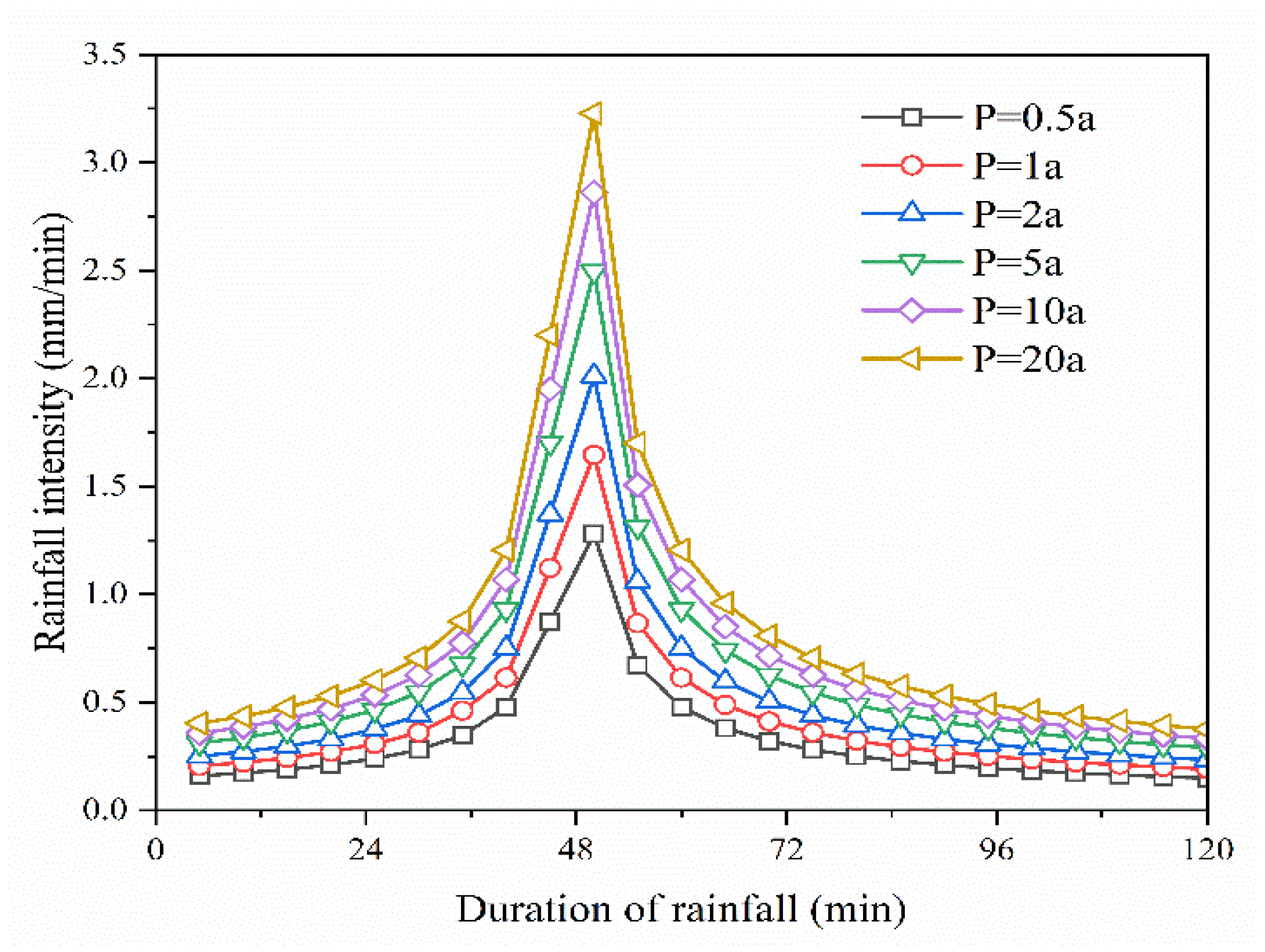
Rainfall Data Selection

Four representative rainfall events with different intensities were selected.

(2)

Selection of Model Parameters and Change Steps

To ensure that the other parameters remained unchanged, eight empirical parameters were selected as the objects based on the initial values of the simulation parameters [24]; 70%, 80%, 90%, 110%, 120%, and 130% of the initial values and debugging of these parameter values. The parameter debugging results are presented in

Table 6. SWMM empirical parameter debugging results.

Parameter Name	Initialization Value	Parameter Debugging Value
		−30%	−20%	−10%	10%	20%	30%
Manning coefficient of permeable zone	0.24	0.168	0.192	0.216	0.264	0.288	0.312
Manning coefficient of impermeable zone	0.012	0.0084	0.0096	0.0108	0.0132	0.0144	0.0156
Maximum infiltration rate (mm/h)	78	54.6	62.4	70.2	85.8	93.6	101.4
Minimum infiltration rate (mm/h)	3	2.1	2.4	2.7	3.3	3.6	3.9
Attenuation coefficient (h−1)	4	2.8	3.2	3.6	4.4	4.8	5.2
Drying time (d)	6	4.2	4.8	5.4	6.6	7.2	7.8
Permeable area depression storage (mm)	5	3.5	4	4.5	5.5	6	6.5
Impermeable area Depression storage (mm)	3	2.1	2.4	2.7	3.3	3.6	3.9

.

(3)

Evaluation Index Selection

The total surface runoff and peak flow rate were selected as sensitivity evaluation indices for the relevant parameters in this study.

Based on the parameter debugging results, the modified Morris screening method was used to study the impact of each parameter on the model under the four measured rainfall scenarios. Scenarios I, II, III, and IV represent light rain, moderate rain, heavy rain, and rainstorm events, respectively. The results of the sensitivity analysis are shown in

Table 7. Sensitivity analysis of four measured rainfall fields on total surface runoff.

Parameter Name	Sensitivity Discriminant Factor S1 of Total Runoff
	27 August 2022 (Light Rain)	13 June 2022 (Moderate Rain)	23 June 2022 (Heavy Rain)	20 July 2022 (Rainstorm)
Manning coefficient of impermeable zone	−0.019	−0.120	−0.170	−0.004
Manning coefficient of permeable zone	0.000	0.000	0.000	−0.013
Impermeable area depression storage	−0.491	−0.086	−0.062	−0.014
Permeable area depression storage	0.000	0.000	−0.015	−0.032
Maximum infiltration rate	0.000	0.000	−0.021	−0.084
Minimum infiltration rate	0.000	0.000	−0.024	−0.021
Attenuation coefficient	0.000	0.000	0.053	0.089
Drying time	0.000	0.000	0.000	0.000

and

Table 8. Sensitivity analysis of four measured rainfall fields to peak surface runoff.

Parameter Name	Sensitivity Discriminant Factor S2 of Total Runoff
	27 August 2022 (Light Rain)	13 June 2022 (Moderate Rain)	23 June 2022 (Heavy Rain)	20 July 2022 (Rainstorm)
Manning coefficient of impermeable zone	0.000	−0.072	−0.086	−0.034
Manning coefficient of permeable zone	0.000	0.000	−0.012	−0.009
Impermeable area depression storage	−0.354	−0.287	−0.030	−0.000
Permeable area depression storage	0.000	0.000	−0.003	−0.046
Maximum infiltration rate	0.000	0.000	0.000	−0.015
Minimum infiltration rate	0.000	0.000	0.000	0.000
Attenuation coefficient	0.000	0.000	0.012	0.072
Drying time	0.000	0.000	0.000	0.000

.

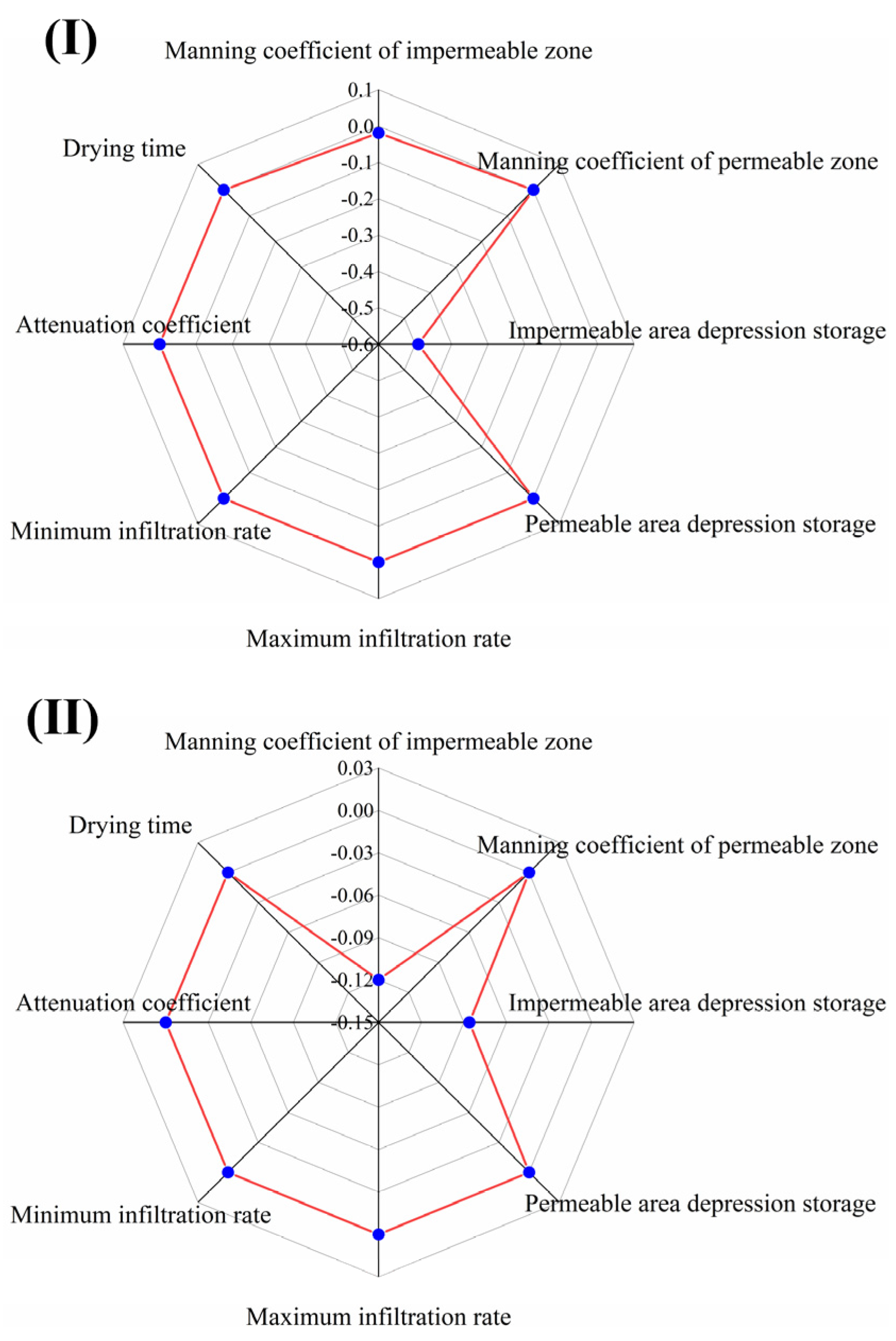
(1)

Sensitivity Analysis of Each Parameter to the Total Runoff under Different Rainfall Conditions

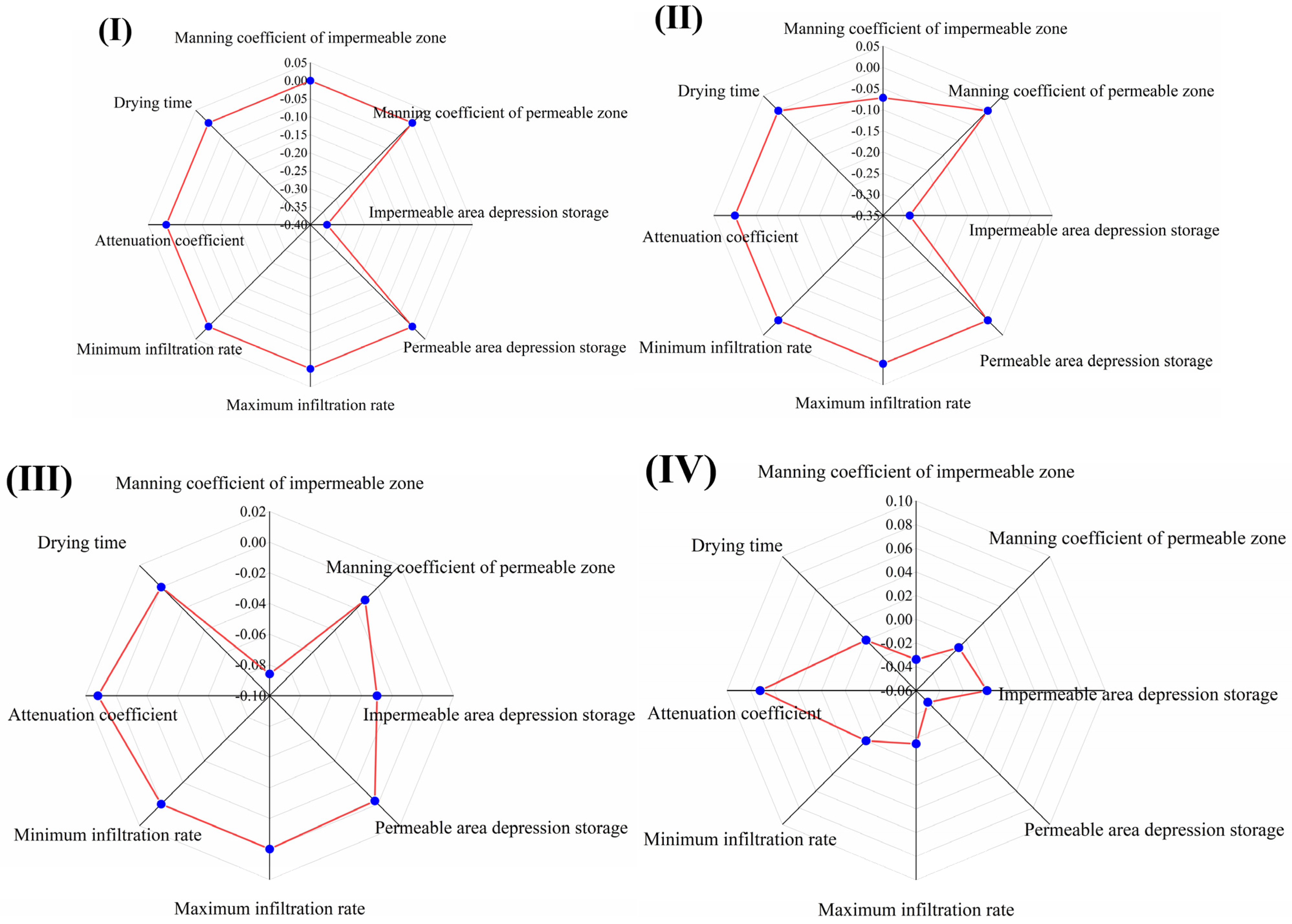
As shown in Figure 5, under different rainfall intensities, the Manning coefficient of the impervious area, impermeable area depression storage, maximum infiltration rate, and attenuation coefficient were sensitive to the total runoff.

The Manning coefficient of the impervious area is moderately sensitive in moderate and heavy rainfall events and insensitive in heavy rainfall events. Under the condition of rainstorm, due to the rapid convergence of the surface, rainwater cannot be infiltrated in time, and all of it is discharged into a water body through a pipeline. When the drainage capacity of the pipe network exceeds its load, overflow will occur, and then change in its parameters will not affect the total runoff value. The low-lying storage in an impervious area only shows insensitivity in rainstorm rainfall events and is a sensitive parameter in other rainfall events, and the absolute value of its sensitivity discriminant factor will decrease with an increase in rainfall intensity. As rainfall intensity increases, the amount of depression storage on the underlying surface will gradually become saturated. If rainfall intensity exceeds a certain value, the parameter will be insensitive. The maximum infiltration rate and attenuation coefficient are only moderately sensitive to the total runoff in the two rainfall events of heavy rain and rainstorm. When rainfall intensity is low, the surface runoff rate is very slow. With an increase in rainfall intensity, the rate of runoff and water storage in a catchment area will gradually be higher than the infiltration rate, which will lead to the formation of surface runoff when the surface rainwater has no time to infiltrate.

(2)

Sensitivity Analysis of Each Parameter for Peak Runoff under Different Rainfall Conditions

As shown in Figure 6, the Manning coefficient of the impervious area, impermeable area depression storage, and attenuation coefficient were sensitive to the peak runoff under different rainfall intensities.

Under different rainfall scenarios, the sensitivity results of the eight model parameters [24] to the total and peak runoff were different; the Manning coefficient of the impervious area, impermeable area depression storage, and attenuation coefficient were sensitive to both the total and peak runoffs, whereas the maximum infiltration rate was only sensitive to the total runoff. The Manning coefficient in the impervious area showed moderate sensitivity in moderate and heavy rainfall events. With a continuous increase in rainfall intensity, surface runoff gradually approaches saturation, and peak flow will not be affected even if the parameters are changed again. The amount of depression storage in an impervious area is moderately sensitive to light rain and moderate rain events, but not sensitive to heavy rain and rainstorm events. It is because of this that the sensitivity of depression storage to peak flow in an impervious area decreases with an increase in rainfall intensity. The attenuation coefficient is only moderately sensitive to peak flow in rainstorm rainfall events. Meanwhile, the other parameters are less than 0.05, all of which are insensitive parameters.

2.3.3. Modelling Rates

Based on the results of the sensitivity analysis, under the return period of a 2-year rainfall, the runoff coefficient method was used to calibrate the eight parameters, including the volume and attenuation coefficient of the impervious area. In this study, the integrated runoff coefficient was 0.599 as the objective function. The coefficient of variation method [25] was used to detect the degree of dispersion between the simulated and actual values, and the single-peak rainfall synthesized by the Chicago Rainfall Pattern was used. The rainfall duration was 2 h and the rainfall return period was 2 years. The parameters were input into the model to obtain the simulated comprehensive runoff coefficients, which were then compared with the comprehensive runoff coefficients of the study area to select a reasonable combination of parameters. The results of the parameter combinations and their simulated runoff coefficients are shown in

Table 9. Parameter rate table.

Parameter Name	Initialization Value	The First Group	The Second Group	The Third Group	The Fourth Group	The Fifth Group	The Sixth Group
Manning coefficient of permeable zone	0.24	0.23	0.22	0.22	0.21	0.2	0.2
Manning coefficient of impermeable zone	0.021	0.015	0.016	0.017	0.018	0.019	0.02
Maximum infiltration rate (mm/h)	79	79.5	80	80.5	81	81.5	82
Minimum infiltration rate (mm/h)	2.5	2.6	2.7	2.8	2.9	3	3
Attenuation coefficient (h−1)	2	2	1.9	1.8	1.7	1.6	1.5
Drying time (d)	6	6	6	6	7	7	7
Permeable area depression storage (mm)	6	6.5	6.4	6.3	6.2	6.1	6.1
Impermeable area Depression storage (mm)	2.5	2.4	2.3	2.1	1.9	1.7	1.5
Runoff coefficient	0.645	0.643	0.633	0.624	0.615	0.607	0.599
Comprehensive runoff coefficient	0.599

.

The optimized Group 6 parameter adjustment results were adopted, and rainfall scenarios under six return periods were simulated [26]. The comprehensive runoff coefficients under five different rainfall intensities were 0.561, 0.575, 0.653, 0.689, and 0.721, respectively. Therefore, the runoff coefficients increased as the rainfall intensity increased. The coefficient of variation method shown in Equation (2) was used to calculate the degree of dispersion between the simulated and actual values and to compare the difference between the simulated and actual comprehensive runoff coefficients. The results of the comparison between the simulated and actual runoff coefficients are shown in

Table 10. Comparison of actual integrated runoff coefficients and simulated runoff coefficients.

Recurrence Period (a)	Rainfall (mm)	Surface Runoff (mm)	Runoff Coefficient	Comprehensive Runoff Coefficient	Variable Coefficient
P = 0.5 a	41.074	23.451	0.561	0.599	6.55
P = 1 a	52.825	30.762	0.575		4.09
P = 5 a	80.111	50.729	0.633		5.52
P = 10 a	93.863	61.358	0.654		8.78
P = 20 a	106.612	72.674	0.681		12.81

.

The coefficients of variation obtained from the simulation of rainfall scenarios in different return periods were all lower than 15%, indicating that the established model could accurately reflect the actual situation. Therefore, applying this set of parameters to simulate the study area is reasonable, and the established model accurately reflects the actual situation.

3. Results and Discussion

The flow, water depth, and flow state of a rainwater pipeline network were simulated for six return periods. The simulation time was set to 6 h (including 4 h of receding time), and the recording time step of the simulation results was 5 min. After the simulation, an operational status summary report, which predicted the risk of urban waterlogging and provided basic guidance for the management of urban rainstorm water flooding, was provided according to the model.

3.1. Surface Runoff Simulation Analysis

The total rainfall, infiltration loss, surface water storage, evaporation loss, and surface runoff were analyzed [27]. The surface runoff simulation data are presented in

Table 11. Simulation results of surface runoff under different return periods.

Recurrence Period (a)	Total Rainfall (mm)	Infiltration Loss (mm)	Surface Water Storage (mm)	Amount of Evaporation Loss (mm)	Surface Runoff (mm)
P = 0.5 a	41.074	16.891	0.732	0	23.451
P = 1 a	52.825	21.250	0.813	0	30.762
P = 2 a	64.575	25.080	0.929	0	38.690
P = 5 a	80.111	28.134	1.248	0	50.729
P = 10 a	93.863	30.782	1.723	0	61.358
P = 20 a	106.612	31.699	1.899	0	72.674

. Evaporation was ignored in the establishment of the production and catchment flow model; therefore, evaporation loss was zero.

The total precipitation, infiltration loss, surface runoff, and surface water storage in the study area increased as rainfall intensity increased, and most of the rainfall was discharged as surface runoff [28]. Therefore, the imperviousness of the underlying surface [29] in the study area was an important factor that increased the surface runoff in the study area.

3.2. Pipeline Operation Simulation Analysis

During rainfall, the dynamic change in water flow in the pipeline network system could have reflected the operation of the storm water pipeline network in the study area. When the drainage volume of the system exceeded the capacity of the storm water pipeline network, water flow would fill up the entire pipe section, and overloading and overflowing would occur in the inspection wells connected to the pipe section.

3.2.1. Analysis of Overloading of Pipe Sections

The operation of the pipelines and the status reports generated by the model were summarized and comprehensively analyzed. The results are shown in

Table 12. Pipeline overloads for different recurrence periods.

Recurrence Period (a)	Number of Overloaded Pipe Segments	Percentage	Number of Pipes Exceeding 30 min Overload Duration
P = 0.5 a	0	0%	0
P = 1 a	9	4.0%	2
P = 2 a	17	7.6%	9
P = 5 a	33	14.7%	12
P = 10 a	36	16.1%	18
P = 20 a	37	16.5%	22

.

As the return period increased, the number of overloaded pipe segments gradually increased, and the overloading time of the pipe segments increased; thus, the load borne by the storm water drainage system increased.

3.2.2. Location Analysis of Overloaded Pipe Sections

To better analyze the overloading situation of the pipeline sections, the operation of the pipeline network in different recurrence periods was visualized and analyzed. The distribution of overloaded pipeline sections in different recurrence periods is shown in Figure 7.

The number of overloaded pipe segments in the study area increased with the return period. Thus, the focus was on the transformation of overloaded pipelines to reduce the risk of waterlogging in the study area.

3.2.3. Analysis of Pipe Section Operation Dynamics

For the overloading of pipeline sections in different return periods, the rainfall conditions in the return period of 5 years were selected, and the operational model was simulated with 20 min as the simulation step. The dynamic display diagram of the pipe network capacity was used to show the operation of pipe sections at different times in the study area. The simulation results are presented in Figure 8.

Figure 8 shows the variation in the instantaneous flow in the drainage network of the study area, and a–f represent the overload of the pipe section at different times: (a) in the first moment (0:20), during which no overloading occurred; (b) in the second moment (0:40), when overloading occurred; (c) in the third moment (1:00), when the rainfall peak was reached and the overloading of the pipe section in the study area became gradually aggravated; (d) although the rainfall intensity gradually weakened in the fourth moment (1:20), the proportion of yellow and red pipe segments was still increasing because the sub-catchment area continued to produce catchment flow; and (e) in the fifth and (f) sixth moments (1:40–2:00), the overloading of the pipe segments in the study area gradually slowed down. The color of the pipe section changed from blue to green, then to yellow, and to red, indicating a gradual increase in the flow rate of the pipe section. Blue indicates the minimum flow rate of the pipe section, and red indicates the maximum flow rate of the pipe section and that overloading occurred.

Based on the above analysis, most of the storm water drainage pipes in the study area could meet the drainage demand of 5-year rainfall.

3.3. Node Overload Analysis

Node overloading implies that the highest water level at a node exceeds the top of the pipe channel; however, no storm water overflow occurs. On the other hand, node overflow occurs when the water depth at the node exceeds the top of the node. Node overloading is typically accompanied by node overflow [21].

3.3.1. Analysis of Node Overloading and Overflow

The node overload and overflow conditions in the study area for the designed rainfall during different return periods were obtained (Figure 9). The red and yellow points are considered overloaded well points. These situations are listed in

Table 13. Node overloads for different recurrence periods.

Recurrence Period (a)	Number of Overflow Well Points	Number of Overloaded Well Points	Percentage of Total Nodes (%)
P = 0.5 a	1	6	1.6
P = 1 a	9	8	4.0
P = 2 a	14	9	5.4
P = 5 a	32	13	10.5
P = 10 a	36	11	11.0
P = 20 a	37	13	11.7

.

It can be observed that the number of overloaded and overflowed checks increased as the return period increased.

3.3.2. Dynamic Analysis of Water Level at Typical Nodes

Based on the analysis of overloading and overflow at the nodes in the study area under different recurrence periods, the nodes prone to overloading and overflow were selected for the specific analysis. Under the design rainfall condition of P = 5 a, the time step of the model simulation was set to 20 min [30]. The SWMM in the study area was run, and the dynamic water [31] levels of some nodes in the road section were displayed in the form of profile diagrams. The results are shown in Figure 10.

Figure 10 demonstrate the dynamics [32] of the water levels at some nodes at different moments: (a) at 0:20, the nodes and storm water pipes in this road section were not overloaded; (b) in the second moment (0:40), some nodes were approaching overload; (c) in the third moment (1:00), when the rainfall peak was reached, overflowing occurred at node J6, overloading occurred at nodes J2 and J22, and the pipe section between J2 and J59 reached its full state; and (d–f) at 1:20–2:00, the amount of rainfall in the study area gradually decreased, and the number of overflow nodes continued to decrease, but due to the large amount of rainwater runoff generated before entering the storm water network, the network still contained a large drainage load. Subsequently, with the gradual discharge of rainfall, the load of the network gradually decreased, and the overloading and overflowing at the nodes gradually subsided.

Graphs of the water level changes in rainwater wells J2, J6, J22, and J59 are shown in Figure 11. When the rainfall lasted until the 50th min, the level of rainwater in well J6 reached the wellhead, and overflow occurred. At this time, water gradually accumulated around the node. During rainfall, the water depths in wells J2 and J22 increased rapidly; nevertheless, the maximum water level did not exceed the depth of the wells, indicating that the two rainwater wells did not overflow.

3.4. Pipe Network System Optimization

3.4.1. Nodal Overflow Control

Based on the simulation results, considering the scenario wherein rainfall occurred once in 2 years as the research object, the overflow situation of the main rainwater wells is presented in

Table 14. Two-year rainfall well overflow data.

Rainwater Well	Corresponding Sub-Catchment Area	Peak Flow Rate (m3/s)	Amount of Water Accumulated at the Node (m3)
J47	S2	1.458	2248
J64	S1	1.667	1828
J154	S11	1.250	1946
J174	S9	1.375	2276
J130	S20	1.375	1936
J90	S26	1.208	1579
J86	S29	1.458	2098
J15	S83	1.375	1248
J118	S74	1.292	1731
J263	S84	1.542	2766
J388	S65	1.417	1601
J426	S25	1.250	1628
J423	S38	1.292	1925

.

There were 13 storm water wells in the study area that had difficulty meeting the drainage demand of a 2-year return period, and overflow occurred. Therefore, if each catchment area meets the storage requirements of the overflow volume of storm water wells within its own boundaries, storm water well overflow and node ponding can be effectively addressed. Low-impact development (LID) [33] facilities are commonly used to reduce storm water flow [34] on-site, thereby improving waterlogging during different rainfall recurrence periods.

The above 13 sub-catchment areas adopted the sunken green spaces in the LID [33] to regulate and store rainfall, and the total storage volume was 26,577 m³. The sinking depth of the sunken green space was set to be 0.2 m, and the scale of the sunken green space facilities [35] in each sub-catchment is shown in

Table 15. Data of sunken green space.

Sub-Catchment Area	Area (m2)	Adjusted Volume (m3)	Sunken Green Area (m2)	Proportion of Sunken Green Space (%)	Reduction Rate of Accumulated Water Volume (%)
S2	429,907	2248	11,240	2.61	54.95%
S1	898,016	1828	9140	1.02	57.06%
S11	337,127	1946	9730	2.88	56.53%
S9	978,140	2276	11,380	1.16	57.50%
S20	187,756	1936	9680	5.15	56.70%
S26	517,411	1579	7895	1.52	58.05%
S29	385,656	2098	10,490	2.72	55.88%
S83	706,477	1248	6240	0.88	56.45%
S74	896,597	1731	8655	0.96	57.43%
S84	536,058	2766	13,830	2.58	55.63%
S65	439,807	1601	8005	1.82	56.76%
S25	271,957	1628	8140	2.99	56.47%
S38	338,762	1925	9625	2.84	58.44%

.

Table 15 shows that the installation of sunken green spaces had a better effect on the reduction in waterlogging, but the area of sunken green space required in the study area was large. Because most of the land types in the study area were dominated by residential and commercial land, the green space area was relatively tight. Therefore, in actual construction, rainwater storage can be performed by combining cisterns, landscape water bodies, and sunken green spaces.

3.4.2. Pipeline Optimization

By analyzing the overloading situation of the pipe sections in the study area, it can be seen that 50% of the pipe sections in Jiulong Avenue (Figure 7) cannot meet the drainage standard under the condition of rainfall with a return period of 5 years; nonetheless, the drainage pipe network in Jiulong Avenue can be optimized by expanding the pipe diameter.

When a pipe diameter reaches its critical condition for overloading, it has the optimal diameter for a drainage pipe [36]. Nine pipes in the area were overloaded, and the results of the pipe diameter optimization are shown in

Table 16. Jiulong Avenue storm water pipe diameter optimization table.

Pipe Number	Optimized Front Pipe Diameter (m)	Optimized Rear Pipe Diameter (m)
126	0.8	2.5
137	1.0	2.0
138	1.2	2.0
139	1.2	2.5
140	1.5	2.0
143	0.8	2.4
145	0.8	2.0
147	1.0	2.8
148	0.8	2.5

. The return period was selected as the design rainfall period of 5 years. The drainage capacity of the pipe before and after optimization is shown in Figure 12. There was no overflow in the optimized pipe section for the drainage of rainfall within 5 years.

Due to the large scope of this study, the sub-catchment area was also large, which had a certain impact on the simulation accuracy of the model. In the future, further subdividing the sub-catchment area could be considered for more detailed and accurate research.

4. Conclusions

In this study, the SWMM was used to simulate [36] the overloading and node overflow of a drainage network under different return periods in the study area located in northern Anhui Province, China. The results revealed that as the return period increased, the surface runoff, the number of overloaded pipelines, and the number of overflow nodes also increased. Moreover, the drainage system in the study area was in good condition. Under a 5-year return period, only 14.7% of the total number of pipe sections were overloaded, and only 13.1% of the total nodes were overloaded. For the area where the overflow node did not meet the 5-year return period, the sunken green space measures in LID control were used to optimize the 13 sub-catchment areas, and the optimized water reduction was more than 50%. The overloaded pipe sections (14.7%) were optimized by increasing their diameter. The optimized pipe diameter was 2 mm or greater, and no overload overflow occurred.

The process of extracting and processing the data of the study area through ArcGIS software10.3 and importing the SWMM is complicated, while the rainstorm drainage and low-impact development simulation system in Hongye can directly use AutoCAD to simulate the low impact development measures. In the future, we can consider combining the SWMM with Hongye to provide new technical support for the promotion of a sponge city. More details of table data can be found in Supplementary Material.