Computational Simulation of Monopile Scour under Tidal Flow Considering Suspended Energy Dissipation

Abstract

Local scour around bridge foundations significantly impacts the stability and safety of marine structures. The development of scour holes adjacent to the pile foundations of sea-crossing bridges, influenced by tidal currents, involves multidimensional physical fields, multiscale coupling, and complex variations in marine loads. However, experimental models alone are inadequate for investigating the underlying mechanisms. Numerical simulation, a critical tool for studying local scour processes, faces the challenge of accurately modeling sediment transport, particularly under tidal flow conditions near pile foundations. To solve this challenge, this research considers the effect of reciprocating flow on sediment shear as well as its characteristic dissipation based on the immersed boundary method, introduces a reciprocating flow dissipation mechanism, and adds a momentum exchange term between the fluid and the sediment to derive a new controlling equation; a new tidal flow localized scour solver is ultimately constructed, termed TidalflowFOAM. The solver effectively simulates complex flow conditions under tidal currents, extending the modeling capabilities to more realistic three-dimensional bridge scour scenarios under combined wave and current conditions. Validation through cases reported in the literature and a series of controlled experiments, encompassing varying depths, flow velocities, and pile diameters, demonstrates the solver’s proficiency in capturing post-vortex data and accurately reflecting the influence of key factors on scour depth. However, the fidelity of the simulated scour hole morphology under tidal flow conditions behind the piles requires enhancement. The proposed numerical model for tidal flow conditions has high solution accuracy and can guide practical engineering applications.

1. Introduction

Pile foundations are widely utilized as the primary support for marine structures such as coastal bridges and offshore wind turbines. However, the bottom of the pile foundation structure faces severe riverbed scour problems. This scouring can undermine the stability and longevity of bridges, incurring substantial economic risks and safety hazards. Scouring around pile foundations, under a variety of hydrological conditions, has become a hot topic in bridge safety research in recent years.

Many scholars have conducted studies on the unidirectional flow problem. In contrast, the marine scour faced by offshore bridge abutment foundations is more complex than unidirectional flow and usually manifests itself in the form of tidal flow [1]. Under the action of tidal currents, the water flows in opposite directions within a given tidal regime, thus causing scour to develop in both directions [2]. This may result in localized scour around the bridge abutments, showing cyclic variations and a more complex scour pattern compared to scour under unidirectional flow. Unidirectional flow scour tends to result in scour holes on only one side of the pile, whereas tidal flow produces large scour depths at multiple locations on the pile. The direction and magnitude of hydrodynamic loads under tidal currents can vary periodically compared to unidirectional flows, and abutment foundations may be subject to different hydrodynamic effects. Tidally induced reciprocal flows may result in reciprocal movement of bottom bed particles. This may lead to rearrangement and localized deposition of sediment on the bottom of the seabed. While sediment scour under tidal flow shows some similarity to unidirectional flow scour, variations in velocity and bathymetry during the tidal cycle may lead to significant differences in scour patterns [3]. Escarameia and May [4] conducted a laboratory study of scour development around different base structures under tidal conditions. They investigated the effects of water depth, structure shape, current direction, and duration of the tidal cycle on the equilibrium scour depth. Tidal flow was simulated using tidal half cycles of different durations and reversal of current direction. Tests with different flow velocities were conducted, and the duration or peak velocity of the tidal half-cycle was matched with that of the constant flow velocity to ensure equal tidal flow. The results show that the equilibrium scour depth of the tidal current increases with increasing live-bed conditions, while the scour depth decreases under unidirectional flow conditions. Jensen et al. [5] compared the scour development of pile foundations under unidirectional and tidal flow, and they noted that the scour depth and the amount of eroded sediment were slightly greater for reverse flow compared to unidirectional flow. McGovern et al. [6] decomposed the tidal signals into three time steps with constant flow rates under clear water, transition, and live bed conditions based on field data. They concluded that the final scour depth of reciprocal flow under live-bed conditions is less than unidirectional flow. Schendel et al. [7] conducted tests of monopile scour by tidal flow and compared the results with those of unidirectional flow tests. The results showed that to accurately estimate the depth of tidal flow scours, it is necessary to increase the unidirectional current flow rate by approximately 15–20% to match the tidal root-mean-square flow rate.

On the other hand, a major difference between tidal flow and unidirectional flow scour is the sensitivity of tidal flow to the KC (Keulegan–Carpenter) number. Sumer et al. [8] conducted a flume test for a cluster of vertical piles under wave conditions, and it was found that scour around the piles under wave conditions was controlled by the tail vortex and horseshoe vortex and that the KC number was the main influencing parameter for equilibrating the depth of scour under moving-bed scour conditions. Whitehouse and Stroescu [9] studied the effect of tidal currents on the scour of a cylindrical monopile under living-bed conditions. They kept the forward and reverse flow rates of the tidal flow constant and changed only the time period of the flow change. The flow change cycle time was found to be a key control on scour. In addition, some scholars have also found that the KC number affects post rear-of-pile-tail vortex shedding and that the post rear-of-pile-tail vortex is one of the important factors influencing the development of post-pile scour [10,11]. However, existing scour models do not take this factor into account, and this variability may lead to significant errors between simulation results and reality.

In recent years, with the development of high-performance computers and the proposal of some improved mathematical models, computational fluid dynamics (CFD) has received more and more attention from scholars. Sediment scour and deposition phenomena around monopiles can be effectively simulated using computational fluid dynamics (CFD) models, which allow for a better understanding of complex scour mechanisms that cannot be directly observed in experiments [12,13,14]. For numerical simulations, considering the use of comprehensive solvers can help improve the simulation accuracy. New numerical techniques or models can be implemented within the framework of OpenFOAM. The high quality of its fluid dynamics solvers and turbulence models, as well as its open source, easy modification, and extension make OpenFOAM a popular tool for studying fluid dynamics. An example is the Eulerian two-phase flow solver SedFoam proposed by Cheng et al. [15]. It considers the multiphase fluid as a mixture of two or more continuous phases and solves the conservation equations for each continuous phase in a Eulerian coordinate system. The model is capable of simulating scour processes around structures with arbitrary geometries, and although reasonable results have been obtained in specific test cases, the drawbacks of using the two-phase Eulerian model for pile foundation scour simulation cannot be ignored. The two-phase Eulerian approach relies on interaction models when describing two interactions, and the parameters in these models often need to be determined from empirical or experimental data with some uncertainty. In addition, there is a huge demand on computational resources because of the need for resource-consuming CFD calculations for water and sediment. In addition, some scholars have used CFD-DEM solvers to study localized scouring of offshore structures [16,17,18]. However, the biggest challenge of local scour studies using CFD-DEM methods is in the modeling of sediment particles, which to some extent demands even more computational resources than the two-phase Eulerian methods because solid phases need to build up a huge order of magnitude of Lagrangian particle counts in the course of the study. This has limited studies to a very small range of simulations; it is therefore worth exploring whether there is room for further development of the flow field in such studies. In summary, neither of these two methods is the best tool for studying local scour in monopiles with tidal flow. Song et al. [19] proposed a three-dimensional scour model based on the immersed boundary method, in which a new wall function is introduced to obtain accurate flow and wall shear stress results; ensuring that wall shear stresses are smooth and accurate is the key to the successful simulation of scour. This method ensures high simulation accuracy with acceptable consumption of computational resources and offers the possibility of further study of localized scour in tidal flow monopiles.

In summary, our review reveals no prior use of OpenFOAM for simulating bridge scour under tidal flow. Consequently, the main goal of this study is to implement and validate a new sediment scour model in OpenFOAM. In this work, we consider the effect of tidal flow on sediment shear as well as its characteristic dissipation based on the IbscourFoam solver in the open-source CFD software OpenFOAM-5.X. Based on a modification of the source code of the solver, the tidal flow dissipation mechanism is introduced, and a momentum exchange term between the fluid and the sediment is added, thus constructing a new local scour solver for tidal flows, TidalflowFOAM. The following sections first introduce the basic conservation equations used. Three unique difficulties in the numerical simulation of tidal flow calculations are then presented, with a targeted discussion of each. The model is validated with numerical results from Whitehouse’s tidal flow experiments, and good validation results are obtained in scour depth as well as flow field simulations. Finally, to further validate the solver model, we conduct several sets of controlled experiments for different water depths, flow velocities, and pile diameters, which are the key factors affecting local scour, and discuss the differences between the experimental scour depths as well as the morphology of scour holes and the simulation results. Finally, the results of the study and future work are discussed.

2. Tidal Flow Bridge-Scour Simulation Model

The solver TidalflowFOAM proposed in this work was implemented in OpenFOAM version 5.X [20]. The fluid-phase solver component utilizes data structures and code functionalities from the foam-extend project within OpenFOAM [21].

2.1. Hydrodynamic Model

This section outlines the development process for the solver’s governing equations. Numerical methods are utilized in CFD to solve equations, since closed-form analytical solutions are limited to very simplistic geometries and flow conditions. The distinction of this work lies in the introduction of two new parameters into the traditional governing equations. The modified governing equations for fluids include the continuity equation and momentum conservation equation. The expressions are shown in Equations (1) and (2):

$$\frac{\partial }{\partial t}\left({\alpha }_f{\rho }_f\right)+\nabla \cdot \left({\alpha }_f{\rho }_f{u}_f\right)=0$$

(1)

$$\frac{\partial }{\partial t}\left({\alpha }_f{\rho }_f{u}_f\right)+\nabla \cdot \left({\alpha }_f{\rho }_f{u}_f{u}_f\right)=-{\alpha }_f\nabla p+\nabla \cdot \left({\alpha }_f{\tau }_f+{\tau }_w\right)+{\alpha }_f{\rho }_{f}g-R_W-R_{f,p}$$

(2)

The subscript $f$ denotes the fluid phase; ${\alpha }_f$ is the volume fraction of the fluid; ${\rho }_f$ is the fluid density; $u_f$ is the instantaneous velocity of the fluid; $p$ is the hydrostatic pressure; $g$ is the gravitational acceleration; ${\tau }_f$ is the fluid stress tensor, ${\tau }_f=-\frac{2}{3}(\mu \nabla \cdot u_f)I+\mu [\nabla u_f+\nabla u_f^T]$, where $\mu$ is the fluid kinematic viscosity and $I$ is a unit tensor; ${\tau }_w$ is the bed stress tensor caused by the tidal flow; $R_W$ is the characteristic dissipation term for tidal flow; $R_{f,p}$ is the momentum exchange term between the fluid and particles. The coefficients ${\tau }_w$, $R_W$, and $R_{f,p}$ are modification factors introduced in the governing equations in this work.

${\tau }_w$ can be expressed as follows:

$${\tau }_w=\frac{1}{2}{\rho }_f{f}_w{u}_0^2$$

(3)

where $u_0$ is the near-bed flow velocity; $f_w$ is the wave friction factor proposed by Soulsby [22], which is given by $f_w=0.993{\left(\frac{1}{KC}\right)}^{0.52}$, where $KC$ is the Keulegan–Carpenter number, which is a dimensionless parameter representing the relative importance of wave inertia and bed resistance forces. It is given by $KC=u_m{T}_o/d_{50}$, where $u_m$ is the maximum tidal flow velocity, $T_0$ is the period of the alternating flow velocity in tidal flow, and $d_{50}$ is the median grain size of the sediment.

The term $R_W$ is the additional kinetic energy dissipation due to the change in flow direction, as proposed by Burcharth and Andersen [23]. Consequently, the consideration is only relevant when simulating conditions under tidal flow.

$$R_W=\left(1+\frac{7.5}{KC}\right)\frac{(1-{\alpha }_f){\rho }_f{u}_f}{{{\alpha }_f}^2{d}_{50}\left|u_f\right|}$$

(4)

The term $R_{f,p}$ is the momentum exchange between fluid and particles [24]. This term is directed opposite to the flow direction of the water and its magnitude is influenced by the shape of the sediment particles. $R_{f,p}$ can be calculated as follows:

$$R_{f,p}=\beta (u_f-u_p)$$

(5)

$$\beta =\left\{\begin{array}{ll}0.75C_d\frac{{\rho }_f\left|u_f-u_p\right|{\alpha }_f{\alpha }_p}{d_{50}}{{\alpha }_f}^{\psi },\hfill & {\alpha }_f<0.8\hfill \\ 150\frac{{\alpha }_p(1-{\alpha }_f)\mu }{{\alpha }_f{d}_{50}^2}+1.75\frac{{\rho }_f\left|u_f-u_p\right|{\alpha }_p}{d_{50}},\hfill & {\alpha }_f\le 0.8\hfill \end{array}\right.$$

(6)

where $\beta$ is the coefficient in the calculation process; ${\alpha }_f$ is the particle volume fraction; $\psi$ is a parameter related to particle volume fraction, which represents the increase of resistance with the increase of particle volume concentration [25]. In this study, the value of $\psi$ is −2.65. $C_d$ is the drag coefficient, as follows:

$$C_d=\left\{\begin{array}{l}\frac{24}{R{e}_p}\left(1+0.15R{e}_p^{0.687}\right), R{e}_p\le 1000\\ 0.44, R{e}_p>1000\end{array}\right.$$

(7)

where $R{e}_p$ is the particle Reynolds number, as follows:

$$R{e}_p=\frac{{\rho }_f\left|u_f-u_p\right|d_{50}}{\mu }$$

(8)

Note that the k-ω SST-SAS model [26] is also included in the solver, and switching between different turbulence models is achieved by setting the turbulence properties dictionary. To close the equations, it is necessary to introduce an additional turbulence model to obtain the turbulent viscosity. This study employs the single-equation LES (large eddy simulation) sub-grid model proposed by Yoshizawa and Horiuti [27] to simulate turbulence. This model decomposes turbulence into eddies of various scales, retaining a certain level of flow field detail. This is particularly helpful for the research presented herein, which focuses on the changes in the flow field turbulence during the flow direction changes within tidal currents. The LES model uses sub-grid scale (SGS) stresses to account for the effects of small-scale vortices, with the equation expressed as follows:

$${\tau }_{ij}-\frac{1}{3}{\tau }_{\kappa \kappa }{\delta }_{ij}=-2{\nu }_{sgs}\overline{S_{ij}}$$

(9)

where ${\tau }_{ij}$ is the sub-grid scale tensor; ${\overline{S}}_{ij}=\frac{1}{2}(\partial {\overline{u}}_i/\partial x_j+\partial {\overline{u}}_j/\partial x_i)$ is the resolved scale strain rate tensor; and ${\nu }_{sgs}$ is the sub-grid eddy-viscosity, as follows:

$${\nu }_{sgs}=c_k△\sqrt{k_{sgs}}$$

(10)

$$\frac{\partial k_{sgs}}{\partial t}+\nabla \cdot (k_{sgs}{u}_f)-\nabla \cdot (D_k\nabla k_{sgs})=G-{\epsilon }_{sgs}$$

(11)

where $k_{sgs}$ is the sub-grid-scale turbulent kinetic energy; $D_k=\nu +{\nu }_{sgs}$; $G={\nu }_{sgs}\left|sym{(\nabla u)}^2\right|$; ${\epsilon }_{sgs}=c_e{k}_{sgs}^{1.5}/△$. Both $c_e$ and $c_k$ are parameters in the process of equation deduction.

2.2. Sediment Transport Model

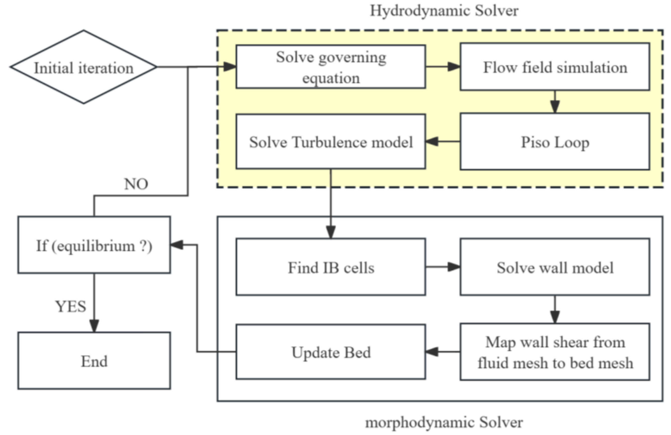
In this study, the scoured riverbed surface was obtained by deforming the immersed boundary: firstly, the sediment layer was modeled as the immersed boundary in STL format (Figure 1), then the parameters obtained from the hydrodynamic solver were substituted into the sediment transport equation to obtain the riverbed elevation, and finally, the immersed boundary was updated to obtain the whole riverbed surface.

A detailed description of the deformation method of the immersed boundary can be found in Song, Xu, Ismail, and Liu [19], which will not be presented in this work, and the sediment transport model used in the manuscript will be described below. The bedload transport rate over a flat depositional layer $q_0$ is calculated using the empirical formula proposed by Engelund and Fredsøe [28]:

$$\frac{q_0}{\sqrt{sgd}d}=\left\{\begin{array}{ll}18.74\left(\theta -{\theta }_{cr}\right)\left({\theta }^{1/2}-0.7{\theta }_{cr}^{1/2}\right),\hfill & if\theta >{\theta }_c\hfill \\ 0,\hfill & if\theta <{\theta }_c\hfill \end{array}\right.$$

(12)

where $s$ is the submerged specific gravity, $s={\rho }_p-{\rho }_f/{\rho }_f$; $\theta$ is the Shields Number; and ${\theta }_{cr}$ is the critical Shields Number.

$$\theta =\frac{{\tau }_s}{{\rho }_{f}g\left(s-1\right)d_{50}}$$

(13)

$${\theta }_{cr}=\frac{0.3}{1+1.2D_{*}}+0.055\left[1-\exp \left(-0.02D_{*}\right)\right]$$

(14)

where ${\tau }_s$ is the near-bed shear stress; $D_{*}$ is the non-dimensional diameter, and it can be calculated as follows:

$$D_{*}={\left[\frac{\left(s-1\right)g}{{\nu }^2}\right]}^{\left(1/3\right)}{d}_{50}$$

(15)

$${\tau }_s={\rho }_f{\left[\frac{\kappa }{\ln \left(d_{50}/12h\right)+1}\right]}^2{V}^2$$

(16)

where $\kappa =0.41$ is the Von Karman number.

Subsequently, the riverbed elevation is obtained by solving the Exner equation:

$$\left(1-n\right)\frac{\partial z_b}{\partial t}=-\nabla \cdot \left(q_0\frac{{\tau }_s}{\left|{\tau }_s\right|}\right)$$

(17)

where $z_b$ is the streambed elevation; n is the porosity of the bed, and it is equal to ${\alpha }_f$ in this work.

2.3. Model Coupling

As shown in Figure 2, the first step is to select the appropriate simulation model depending on whether the simulation conditions include tidal flow or not. Because the k-omega SST SAS model does not include any of the three terms if the Tidal Flow Bridge-Scour Simulation model is selected, then all three terms participate in each time step iteration as part of the governing equation. The PISO (Pressure-Implicit with Splitting of Operators) algorithm is employed for velocity–pressure coupling, yielding the distribution of velocity and pressure for the next time step. Subsequently, the model determines the bed elevation through the bed shear stress and sediment transport equations. The solving process is specifically divided into the following four parts:

• At the beginning of each time step, initial iterations are conducted. The hydrodynamic module computes the fully developed flow field to obtain the fluid’s velocity and pressure fields.
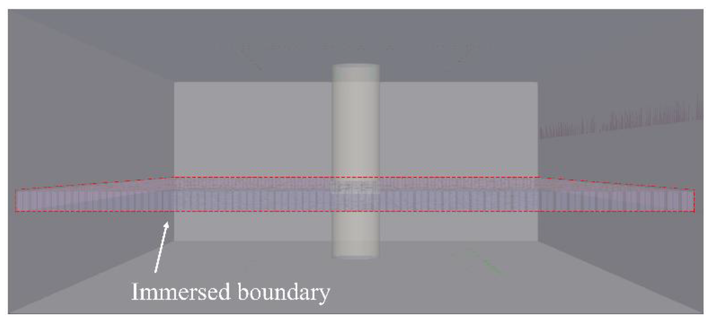
• Wall shear stresses at the immersed boundaries are obtained through the wall function model, and the wall shear forces at the riverbed mesh centers are determined via interpolation.
• The sediment transport equation is calculated to obtain the sediment transport rate, and the Exner equation is solved to update the riverbed elevation.
• After obtaining the new riverbed surface, the above process is repeated until the scour reaches equilibrium.

3. Validation of the Tidal Flow Model

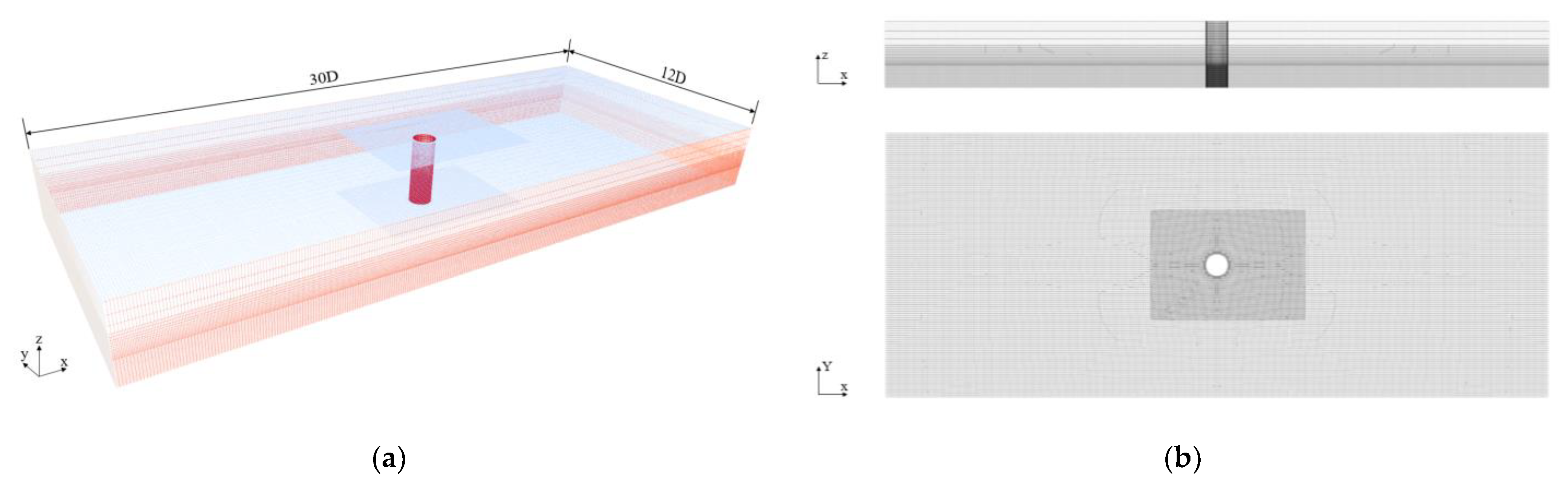
Based on the mathematical model presented above, the following sections address several important simulation challenges in building an accurate tidal flow scour model. The first is how to build the grid model, the second is the model boundary condition setting, and the third is how to implement the tidal flow simulation.

3.1. Mesh Setup

In this section, the process of establishing the validation model is presented. Overall, the establishment process consists of three parts: (1) mesh setup; (2) boundary condition setting; and (3) simulation of the tidal flow field.

3.2. Model Mesh Settings

In the experiment, the pile has a diameter of 0.114 m, the median sediment grain size is 0.17 mm, the flow velocity of the water is 0.381 m/s, and the water depth is 1.14 m. The computational domain used for the numerical simulation is shown in Figure 3. Based on the research by Akhtaruzzaman Sarker [29], the flow field approximately 12D away from the pile center can be considered unaffected by the pile. Therefore, to save on model size, the total length of the model is set to 30D and the width to 12D, with a certain distance reserved at the front and back to allow the water flow to fully develop and stabilize. The grid is locally refined around the pile to better capture the details of the scour hole, and three different grid resolutions are used vertically, which is one of the advantages of OpenFOAM, allowing for varying grid resolutions in different computational domains. During computation, each domain is simulated independently, and then the structures are consolidated during the merging process, ensuring accuracy while saving on computational resources. The total number of grids in the model reaches 4,080,000.

3.2.1. Boundary Conditions

The model boundary conditions are set as follows:

• At the inlet, the velocities in the y-direction and z-direction are set to zero, and for pressure p, turbulent kinetic energy k, and turbulent viscosity μ, a zero-gradient condition is applied. In this study, the OpenFOAM plugin swak4Foam with the funkySetFields function is used to define the initial flow velocity, which can be used to set up an initial flow field with a certain spatial distribution. The velocity profile is determined based on the logarithmic law, as follows:

$$u_x\left(z\right)=\frac{u_f}{\kappa }\ln \left(\frac{30z}{\mathsf{\Delta }}\right)$$

(18)

where $u_f$ is the friction velocity; Δ is the roughness of the riverbed, usually taken as 2.5 times the $d_{50}$.

2.

At the outlet boundary, except for the pressure, all quantities are specified with a zero gradient condition $\left(\partial /\partial n=0\right)$, and pressure is specified with the total pressure condition $\left(p_0=0\right)$.

3.

At the top surface, the slip condition $\left(u\cdot n=0\right)$ is specified for the velocity, and zero gradient conditions are specified for p, v, and k.

4.

At the bottom and pile wall surfaces, a no-slip condition is specified for the velocity $\left(u\cdot n=0, ut=0\right)$, and zero gradient conditions are specified for p. The boundary conditions are specified using the wall function in OpenFOAM.

5.

At the sidewall surface, a symmetry condition was set for all variables.

Parameter settings in the calculation are shown in

Table 1. Summary of simulation parameters.

Simulation Parameters	Value
Sediment Density	2650 Kg/m3
Sediment Diameter	0.17 mm
Shape Factor	1
Fluid Density	1000 Kg/m3
Fluid Dynamic Viscosity	8.90 e−4 Pa·s
Time Step	2 × 10 −4 s

. The key parameter MaxCo number directly affects the stability of the solution as well as the accuracy of the calculation; in order to be conservative, it is set to 0.5, and the time step of the solution is 2 × 10 ⁻⁴ s. In order to represent the effect of tidal flow dissipation on scour depth, two sets of numerical simulations were conducted, one considering the KC number and the other turning off the tidal flow dissipation function. A 72-core processor was used for the computation, with an average time of 12 h for 1 s. The new solver does increase the simulation time, which is about 20% more than the solver without the modifications. For practical applications, we think the increased computational load and run times are acceptable.

3.2.2. Tidal Flow Realization

After defining the boundary conditions of the model, another focus of this study is the simulation of tidal flow in OpenFOAM. Tidal flow, as a flow phenomenon characterized by periodic changes, has its flow direction altered periodically. In numerical simulation, this means that the boundary conditions require further processing. Considering the periodic characteristics of the tidal flow, it is necessary to set boundary conditions that can change with time. In this work, the author adopts the concept of segmented calculation to simulate tidal flow. The conventional inlet and outlet boundaries are defined as timeVaryingUniformFixedValue, and the swapping of the inlet and outlet boundaries is controlled by time data. It is assumed that the direction of the tidal flow changes only once within one cycle. After simulating half a cycle with the same flow direction, a result file is generated. A Python-based tool library, fluidfoam, reads the velocity and pressure field data from this result file and introduces them as initial conditions for the next cycle of the flow field. By treating half a cycle of a constant flow velocity as a call cycle for the flow field, new computational time steps are established whenever the flow direction changes, and the velocity and pressure fields from the previous time step are used as initial conditions for the new time step, achieving the periodic change of flow velocity in the numerical simulation.

Figure 4 shows the velocity in front of the pile after the full development of the water flow. The flow velocity and period settings for the simulation case follow the settings of Whitehouse et al. [9], with a flow velocity of 0.381 m/s and a complete tidal flow period of 114.3 min. The simulation case runs for a duration of seven cycles.

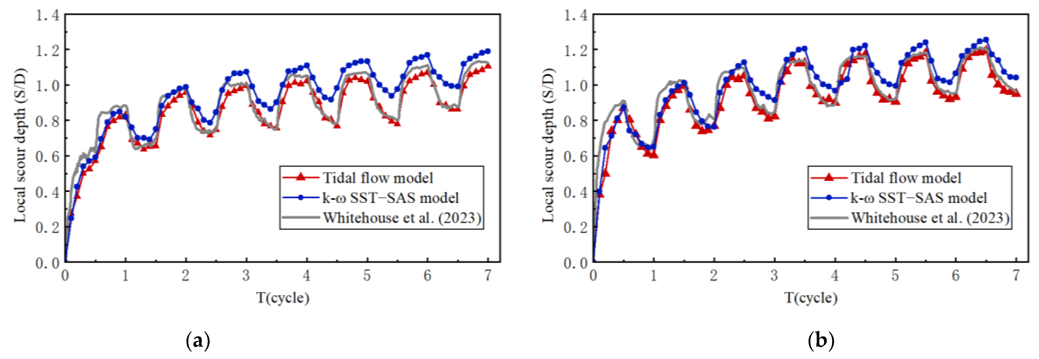
3.3. Verification of Local Scour Depth

To eliminate the effect of pile diameter, the relative scour depth (S/D) is obtained by dividing the actual scour depth (S) by the pile diameter (D). The relative scour depth (S/D) results of the pile (front and rear) for the validation calculations are shown in Figure 5, which shows a progressive scour model that tends to an equilibrium value, both in front of the pile and in the rear of the pile, under the action of a special flow field such as the tidal flow. An important difference between tidal flow scour and unidirectional flow scour is reflected in the backfilling of sediment around the bridge abutments. According to Kumar et al. [30], in the case of live-bed scour, localized scouring occurs when the shear force of the water flow on the bed sediment is greater than the critical starting velocity of the sediment, and the foundation of a bridge under unidirectional flow scour conditions is in a locally scoured state for the majority of the time. The bridge foundation under unidirectional flow scour conditions is in a localized scour state most of the time; however, under tidal flow conditions, since the flow velocity is constantly varying, it is not ensured that the flow scours the streambed all the time, and the sediment scour depth will be less than under unidirectional flow conditions due to the presence of siltation. Previous studies on scouring under unidirectional flow have generally considered ejection and scouring due to wall turbulence near the pile to be the main factors in sediment particle transport [31,32]; the pattern of scouring under tidal flow is more complex in comparison.

From Figure 5a, it can be seen that the simulation results of pile front scour are more consistent with the experimental data; the maximum relative scour value in seven cycles is −1.193, and the maximum scour value in front of the pile in the Whitehouse experiment is −1.209; the relative error between the two is only 1.3%. In the first half of the first cycle, the sediment in front of the pile was flushed rapidly; at this time, the main driving force of sediment transportation in front of the pile is that the water flow in front of the pile encounters the pile blockage, forming a sinking water flow and rolling up the sediment in front of the pile. It can be seen that in the second half of the cycle, the scouring speed of the sediment in front of the pile is significantly accelerated due to the formation of a more enhanced horseshoe-shaped tail vortex in front of the pile by the reverse flow. The peak scour in front of the pile in the first cycle is 0.87, which is 72.9% of the maximum scour depth. This is similar to the experimental results obtained from the tidal flow experiments of [7], although their experiments used different pile diameters as well as different water depths; the peak scour in the first half of the cycle in the live-bed scour experiment reached 70.2% of the equilibrium scour depth. Comparing the peak scour in the first cycle with the scour valley after the return of sediment in front of the pile, the scour valley after the first return is 0.603, which is 69.3% of the peak scour. Comparing the scour peak to the scour valley in the last cycle in the same way, the ratio is 79.6%.

From Figure 5b, it can be seen that the simulation results in the rear of the pile in the first cycle are smaller than the experimental data, which may be due to the turbulence distribution under the simulation of the flow field at the beginning of the scour and the experimental situation having some differences; however, after a few cycles, the simulation results match well with the experimental data, with the flow field already having been developed completely. The simulated maximum relative scour value is −1.085, and the maximum scour value behind the pile in Whitehouse’s experiment is −1.132, with an error of 4.33%. The simulated peak value of scour in the rear of the pile in the first cycle is 0.824, which reaches 74% of the maximum scour in the rear of the pile. In addition, in the first cycle, the valley of scour is 0.63, and the ratio of the valley of scour to peak value is 75.2%. In the same way, comparing the last cycle, the scour valley/peak ratio is 78.04%. In the comparison, it can be observed that the maximum scour value in the first cycle reaches about 70% of the final scour value both before and in the rear of the pile. The following conclusions can be obtained in the above study comparison:

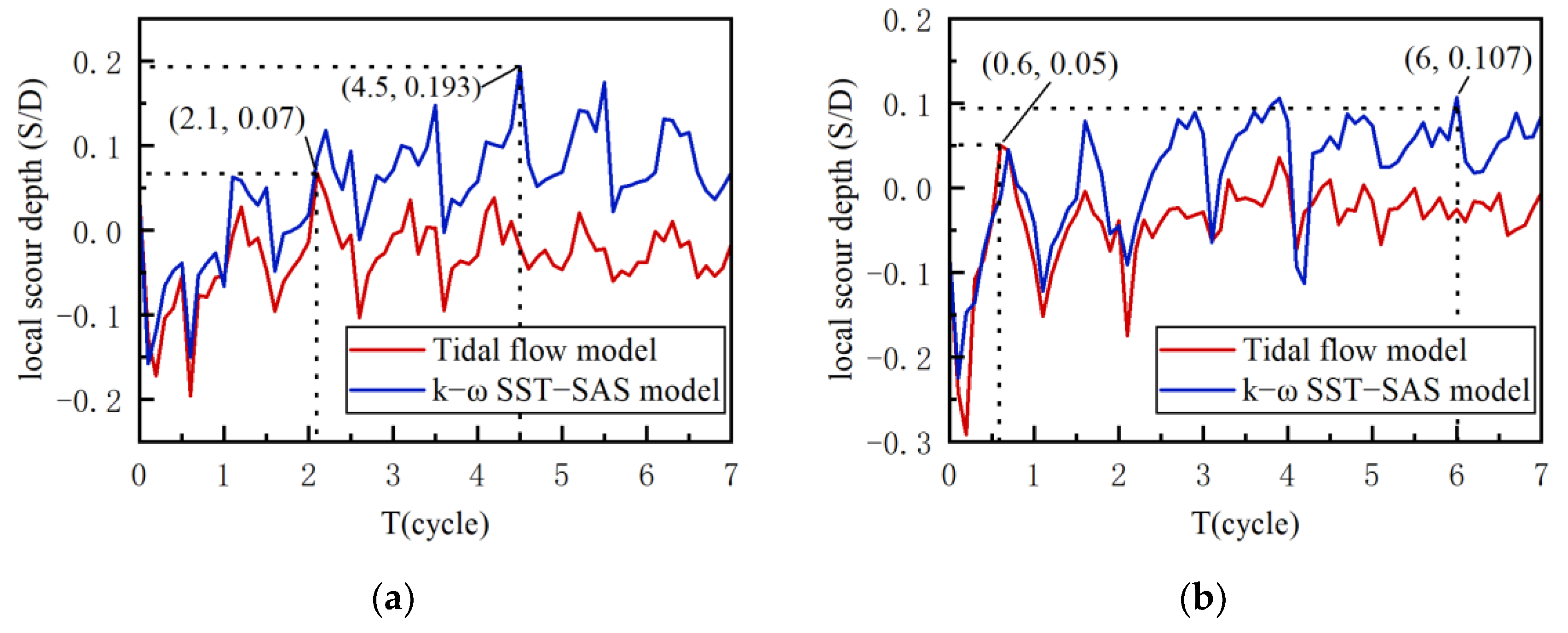
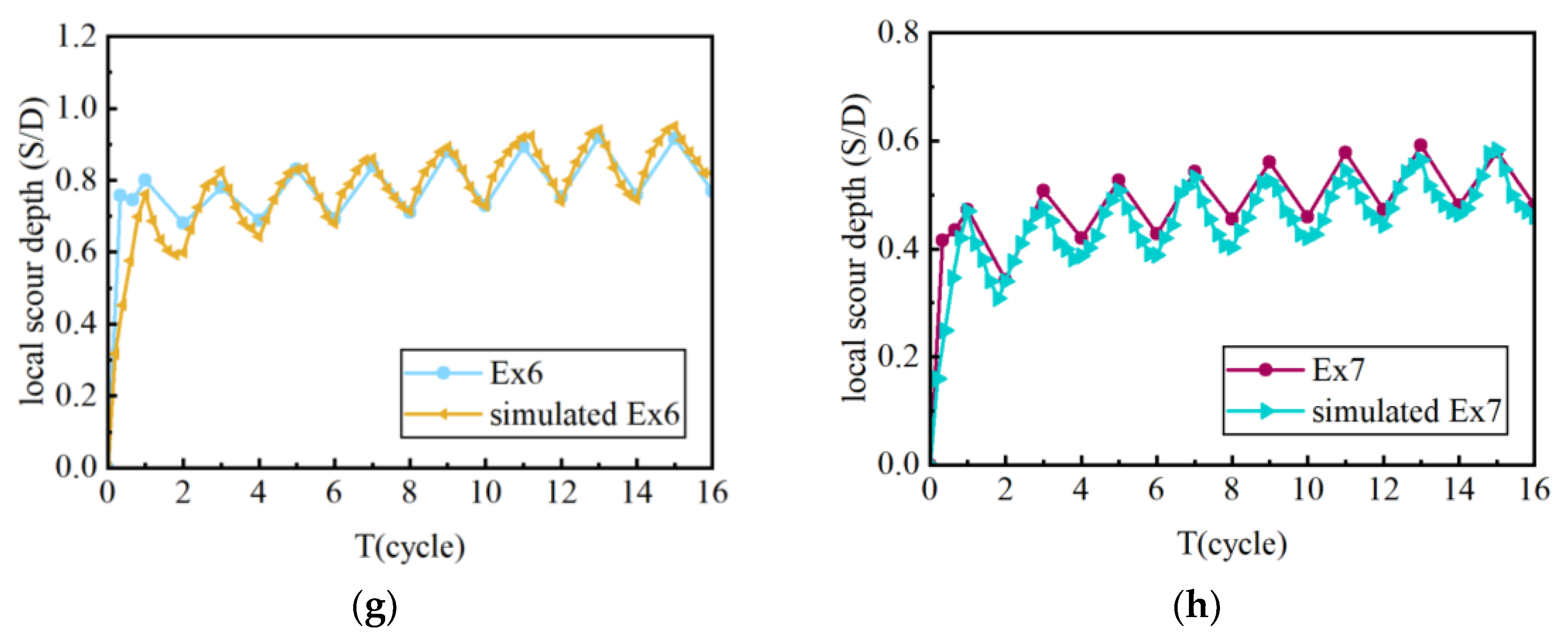
• Similar to unidirectional flow, the location of maximum localized scour in a single cycle under tidal flow conditions occurs in front of the pile. The scour depth in front of the pile is always greater than in the rear of the pile in almost every net cycle. The relative scour depths in front of the pile and in the rear of the pile are not exactly “mirror images”, although the flow velocity varies over the same period of time in the simulation, which may be due to the hysteresis of the flow velocity change. Although the experiments changed the flow velocity at the same time intervals, the change in flow velocity did not lead to an immediate change in the flow direction, and according to the setup in Chapter 2, the fluctuation of the previous flow direction still had an effect on the sediment in the current flow direction. Therefore, this phenomenon clearly indicates the existence of a correlation between flow intensity and scour depth.
• The phenomenon of scour valley/peak ratio increasing with time development was observed both before and in the rear of the pile, which indicated that the development of maximum scour depth under tidal flow conditions was not at the same rate as that of backfilling sediment.
• The development of the scour prior to scour under tidal flow is rapid, and the scour depth can reach about 70% of the maximum scour depth in the first cycle.

Meanwhile, observing the modeling results obtained using the k-ω SST-SAS model without considering the effect of the KC number in Figure 5b, it can be found that the final scour results both before and in the rear of the pile produce large error values. The simulated values obtained using the tidal flow scour model and the k-ω SST-SAS model in front of the pile and in rear of the pile, respectively, are subtracted from the experimental data of Whitehouse to obtain the error values of the two with the experimental values; the errors are plotted in Figure 6. Among them, Figure 6a shows the error values before piling, and it can be seen that the maximum error between the simulated and experimental values obtained from the newly proposed tidal flow scour model is 0.07, while the maximum error of the traditional k-ω model without considering KC dissipation is fully 0.193; however, the two errors do not differ much within the first cycle, which may be mainly due to the fact that the scouring is a unidirectional flow scouring stage in the first cycle. This may be mainly due to the fact that in the first cycle, the flushing is a unidirectional flow stage, so the dissipation caused by the change of flow direction is not reflected in the first cycle, and as the flushing develops, the error caused by this dissipation value becomes more and more obvious. This is a side effect of the fact that the tidal flow scour is more complex than the unidirectional flow scour. Observing Figure 6b, it can be seen that the simulation results obtained by using the tidal flow model still result in a low error value, with a maximum error of 0.05, while the simulation results of the traditional k-ω model, although better compared to the pile front, still have a maximum error value of 0.107. However, the maximum location of the localized scour of the bridge abutment generally occurs in the front of the pile, and therefore the accuracy of the scour in the front of the pile is more important than that in the rear of the pile. Therefore, it can be seen from the above analysis that the dissipation considering the change of flow direction is necessary for the simulation of tidal flow scour. The inclusion of the new dissipation mechanism can effectively reduce the simulation error. Additionally, the traditional k-ω model simulating unidirectional flow scour exhibits better performance.

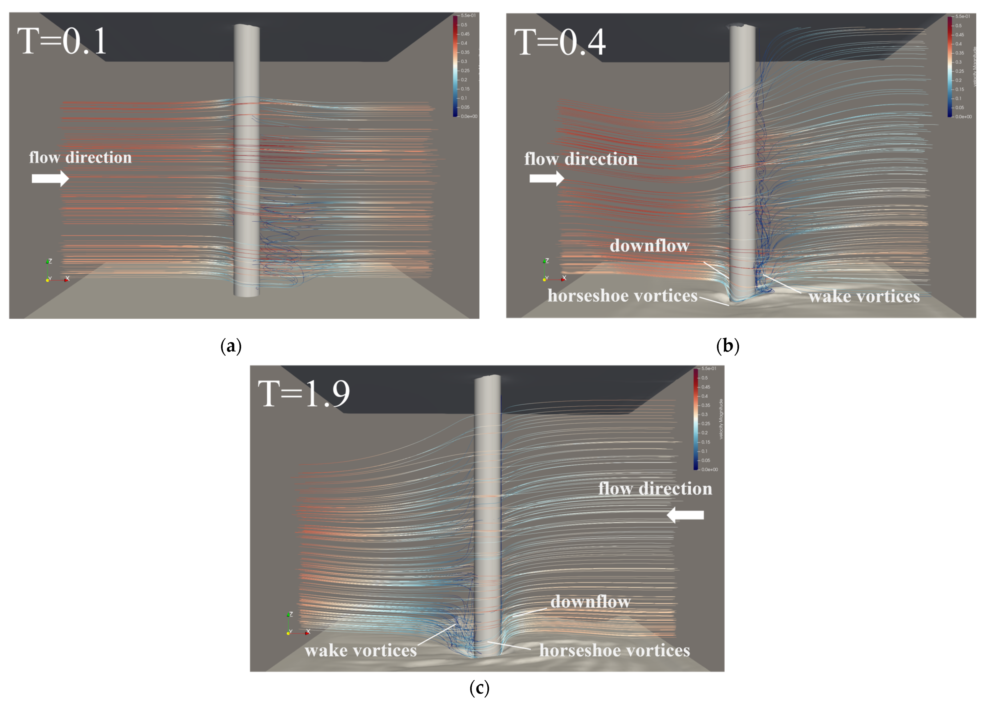
3.4. Verification of Flow Field

For the local scour under tidal flow, it is crucial to accurately simulate the flow distribution around the pile for the simulation of scour depth. Therefore, this work focuses on three representative time points, namely the initial scouring, the middle of the unidirectional scouring stage, and the middle and late stages of the tidal scouring stage, to study the characteristics of the flow field around pile under the tidal flow. Figure 7 shows the flow line diagrams of the flow field around the pile at these three different moments. After the flow field is fully developed, an obvious horseshoe-shaped vortex appears soon after the pile. Figure 7a shows the flow streamlines at T = 0.1, when scouring has just started and the riverbed can be regarded as a flat surface. It can be seen that the sinking current in front of the pile is not obvious, and the flow field appears when the flow in front of the pile reaches the front of the column with a logarithmic flow profile; the difference in flow velocity in front of the pile gradually induces a counterpressure gradient, and the sinking current appears when there is a certain development of the scour hole. It can be seen that the post-pile tail vortex has different intensities at different water depths. Figure 7b shows the streamlined diagram of the flow field around the pile at the moment of T = 0.4, which is the stage of rapid development of the scour hole; however, it is still a unidirectional flow scouring state because the flow velocity has not yet been reversed. However, the intensity of the sinking flow in front of the pile is much stronger than that at the beginning of the scour. Figure 7c shows T = 1.9, when the flow direction of the flow field has completed the reversal change and a new horseshoe-shaped vortex system is formed behind the pile along the negative direction of the x-axis. Although the flow velocity at this time is the same as that in Figure 7b, the difference in the shape of the scouring hole before and after the pile has an obvious effect on the tail vortex, because the scouring around the pile has not yet reached the equilibrium state at this time; thus, there is a great difference in the angle of the scouring hole before and after the pile, and this difference in the angle produces different sizes of the backpressure zone and manifests itself as a difference in the angle of the diffusion of the tail vortex after the pile at the same average flow velocity. A detailed discussion of scour hole angles can be found in Section 5.2 The wake vortices are shed alternately with irregular near-bottom vortices, and as the flow field develops, the post-pile wake vortices enter a steady state of shedding.

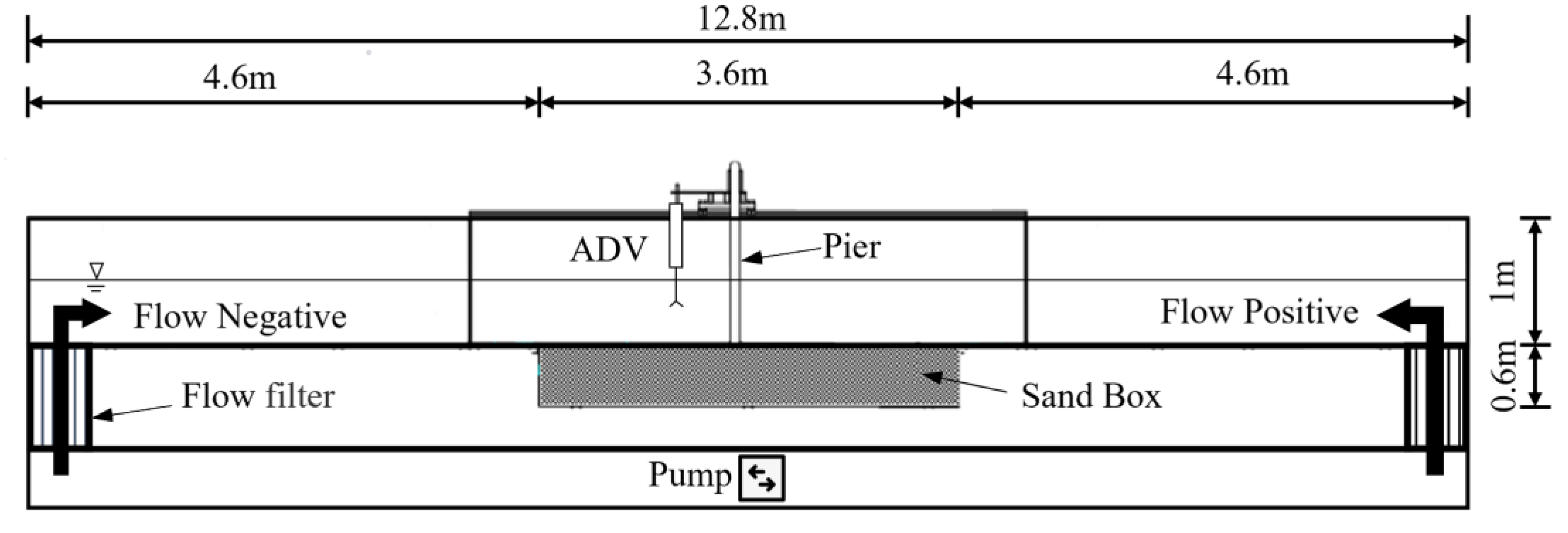
4. Experimental Setup

To further validate the accuracy of the proposed solver and to ensure the authenticity of the data, this study was augmented with flume conditions and multiple sets of control experiments targeting key factors in scour. These experiments encompass a range of water depths, flow velocities, and sediment particle sizes.

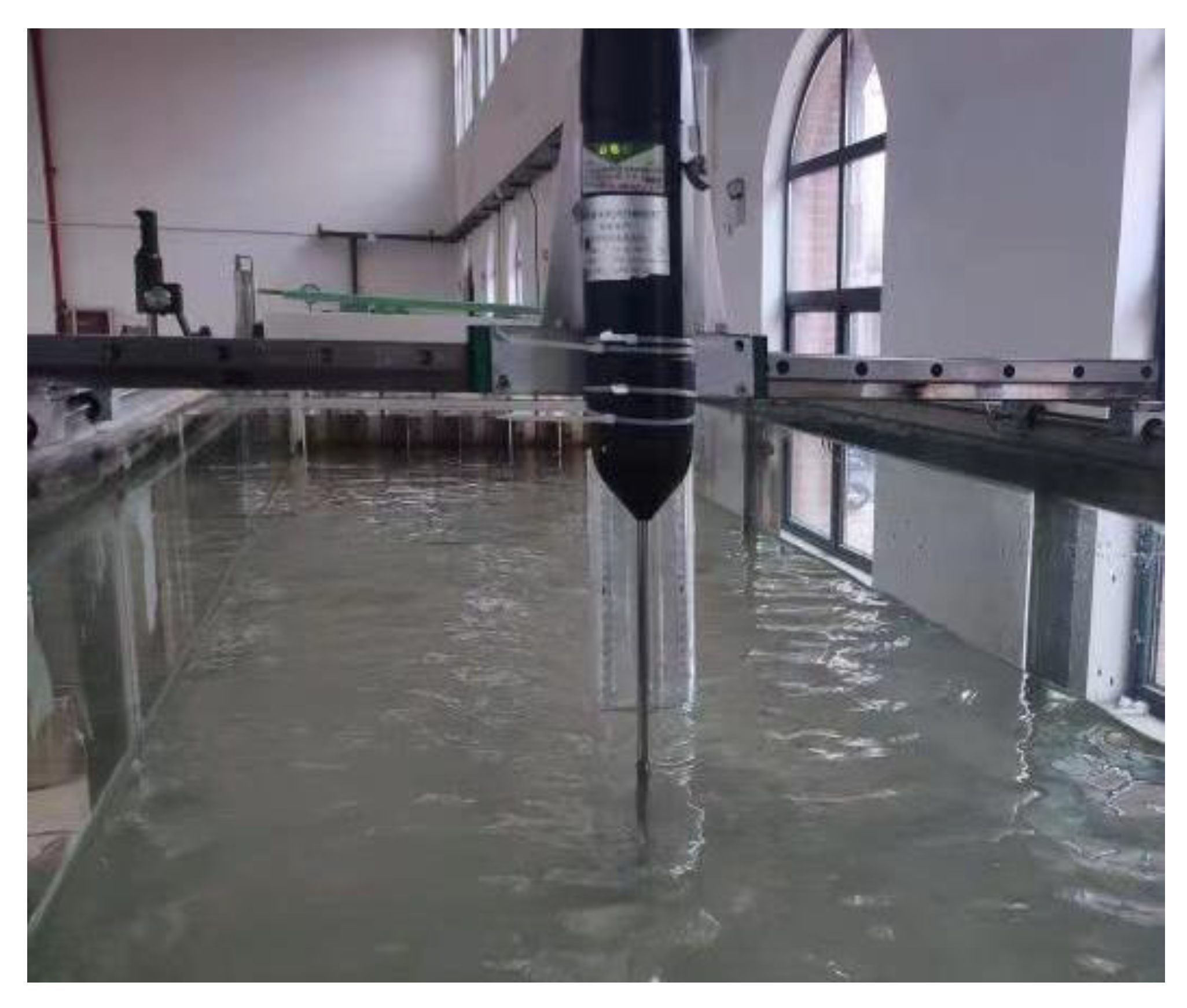
4.1. Experimental Equipment

The experiments are conducted in a flume that is 12.8 m long and 0.7 m wide, with a sediment box in the middle section measuring 3.6 m in length, 0.7 m in width, and 0.6 m in depth. As shown in Figure 8, the flume is driven by a pump system consisting of a pipeline pump and a deflection butterfly valve. The side walls and bottom of the flume are made of transparent tempered glass, and rulers are affixed to the flume walls for reading the water depth and observing the flow state of the water. Above the flume, there is a movable rail on which data acquisition equipment can be mounted. The pile is simulated using plexiglass and is placed at the center of the flume. According to the research by Whitehouse [2], the ratio of the pile diameter to the flume width should be less than 1:6 to minimize the impact of blockage effects. In this experiment, two different specifications of piers are used, ensuring that their blockage ratio is within the range of 1:6; thus, it can be assumed that the scour is not affected by it. To facilitate the reading of scour depth, scale markings are affixed to the pile walls at 0°, 90°, 180°, and 270° in the direction of the incoming flow. In this experiment, the scour depth is measured using a ruler. A sediment box measuring 1.8 m in length, 0.7 m in width, and 0.3 m in height is located at the center position of the flume. In this experiment, the sediment particle size is not one of the subjects of study; therefore, a standard fine sand with a median particle size of $d_{50}=0.16$ mm and a density of $\rho =2.65$ g/cm³ is used. The sand coarseness $D_p/d_{50}=375$ far exceeds the critical value of 50 proposed by Ettema [33]; therefore, it can be considered that local scour around the pile is independent of the sediment diameter. As shown in Figure 9, to ensure the accuracy of the scour flow velocity measurement, Acoustic Doppler Velocimetry (ADV) is used to monitor the flow velocity in front of the pile by placing the probe point at the half position of the water depth for continuous measurements at a sampling frequency of 10 Hz and placing it at the corresponding position behind the pile when the flow velocity is reversed.

4.2. Test Conditions and Methods

As shown in

Table 2. Parameters for the test conditions.

Experiment	H (m)	V (m·s−1)	${\mathit{D}}_{\mathit{p}}$ (m)	${\mathit{d}}_{50}$ (mm)	T (min)
1	0.3	0.35	0.06	0.16	30
2	0.3	0.4	0.06	0.16	30
3	0.3	0.4	0.08	0.16	30
4	0.35	0.25	0.06	0.16	30
5	0.35	0.3	0.06	0.16	30
6	0.35	0.35	0.06	0.16	30
7	0.35	0.25	0.08	0.16	30

Note: H is the water depth; V is the flow velocity; $D_p$ is the diameter of pile; $d_{50}$ is the median particle size of sediment; and T is the cycle time of flow reversal.

, seven sets of dynamic bed scour flume tests under different operating conditions were conducted in this work. Among them, test 4 was used as a standard group and used as a research object for the following study on the scour hole morphology. Yao et al. [34] concluded that the scour depth increases with the increase of the water depth until a critical value of H/D = 4. Therefore, two different heights of water depths were selected for this study, in which ex1 and ex6 corresponded to H/D = 3.75 and H/D = 5.83, respectively, in order to study the effect of different water depths on scour. Due to the limitation of the pump capacity, four lower flow rates of 0.25, 0.3, 0.35, and 0.4 were used in this experiment to ensure that the period of flow rate change could be accurately controlled.

To ensure the reliability of the comparison, the equilibrium scour depth prediction equation proposed by Sumer et al. [35] was used to fit the final equilibrium scour depth of the test.

$$S_e=S[1-\exp (\frac{-t}{T^{*}})]$$

(19)

where $S_e$ is the final equilibrium scour depth; t is the scour time; and $T^{*}$ is the time scale of the scour.

$$T^{*}=\frac{D^2}{{[g(s-1)d^3]}^{1/2}}\frac{1}{2000}\frac{h}{D}{\left[\frac{u_{\ast }^2}{g(s-1)d_{50}}\right]}^{-2.2}$$

(20)

where $u_{*}=\sqrt{{\tau }_b/{\rho }_f}$ is the shear velocity; and ${\tau }_b$ is the bed-shear stress calculated by TKE methods [36].

The arrangement of this experiment is summarized as follows:

• Pre-preparation stage: Wash the sand to remove impurities, and screen the sand with a sieve to ensure the uniformity of particles. First, install the pile under test conditions on the base of the sedimentation box by bolts to make sure it is firm. Then, spread the sand over the box and inject a small amount of water into the box with the valve open to allow it to soak for 24 h to ensure that it is saturated with sand; then, smooth the sand bed using a scraper.
• Recalibrate the sand bed for levelness prior to the start of each test, and record sediment elevation readings at this time; protect the bed from early scour by pressing two PVC boards into the bed around the abutment prior to water injection.
• Slowly inject water from both sides of the sediment bed to the test water depth H, and dynamically control the flow rate V in the tank by simultaneously controlling the pumps and valves in the tank to achieve the test conditions.
• Carefully remove the PVC covers around the abutments while recording the test start time. The flow rate change cycle is 30 min for each set of tests, and each set of tests is conducted for 8 h. Record the scour depths in the four directions of 0°, 90°, 180°, and 270° from the pile in the direction of incoming flow at 10 min intervals for the first 30 min of scour initiation, and take readings at 30 min intervals thereafter. Subtract the initial scale value from the reading at each moment to obtain the scour depth at that moment.
• At the end of the test, slowly drain the water from the flume, and take final measurements of the local scour holes around the pile.
• Remove sediment in the flume that washed out of the caisson, replace the pile model, and replenish quartz sand upstream of the scour hole in preparation for the next set of tests.

5. Results and Discussion

The solution accuracy of the numerical simulation for scour depth is crucial, and the solution accuracy of TidalflowFOAM was preliminarily verified in previous validation calculations. In order to better study the simulation accuracy under different influencing variables for scour, this work further conducts several sets of flume tests to investigate the influence of key factors on the simulation of tidal flow scour.

5.1. Tidal Flow Experimentation

Based on Melville and Chiew [37], equilibrium was considered to have been reached when the change in scour depth is less than 5% of the pile diameter in 24 h. Although this criterion was not reached in this test, observation of the test data of each group revealed that the maximum scour depth change rate was close to flat, indicating that the scour was close to equilibrium.

Local scour depth (S/D) was obtained by dividing the simulation results and measured data by the pile diameter and comparing the results. Figure 10a shows a summary of the maximum scour depths of the seven groups of tidal flow scour tests, and the comparison of the experimental data with the numerical simulation data for each group is plotted in Figure 10b–f. It can be seen that the simulation data for each group of working conditions match well with the experimental data. Among them, the simulation results of Case 4 and Case 5 have some errors in the early stage, which may as a result of the same issue experienced in the comparison of the previous validation algorithms. However, in some of the simulated cases, the development of scour depth in the early stage of scouring was shifted from the experiments, which may be due to the errors caused by manual readings. The equilibrium scour depths obtained from the fitting of each group of conditions are shown with the simulation results in

Table 3. Comparison of equilibrium scour depth for each test condition.

Experimental Case	Measured S/D	Simulated S/D	Error (%)
1	0.836	0.834	−0.01
2	1.089	1.041	−4.41
3	0.902	0.851	−5.65
4	0.621	0.583	−6.12
5	0.890	0.857	−3.71
6	1.052	1.010	−3.99
7	0.521	0.487	−6.53

, in which the simulated value of condition five has the largest error with the measured value, with an error value of 5.28%; and the smallest error, in condition seven, is −0.02%. Overall, the errors of the equilibrium scour depths for all the conditions are controlled within 6%, which further validates the accuracy of the new tidal flow scour model. It also proves that the new tidal flow scour performs well for all the cases under changing scour factors.

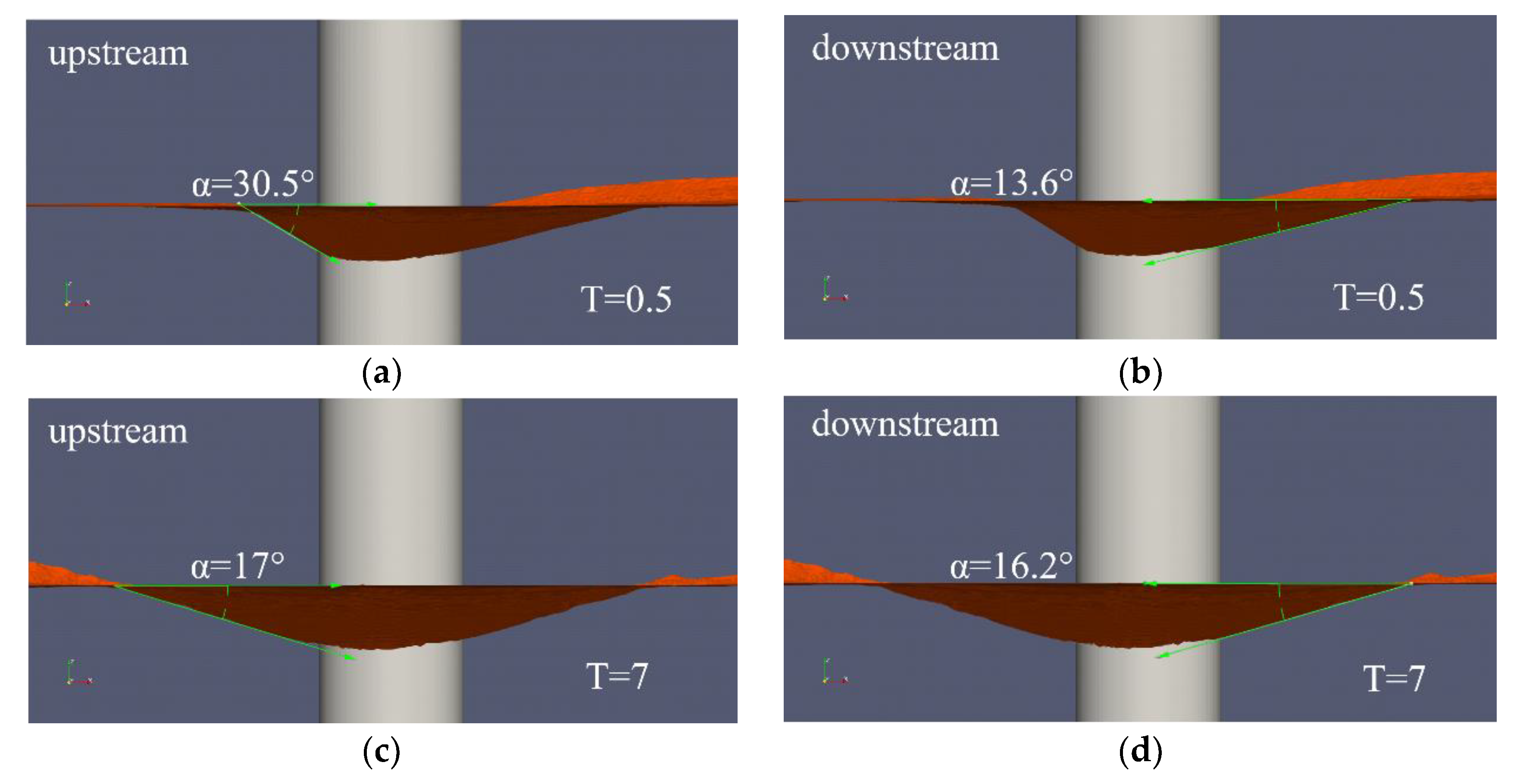
5.2. Verification of Scour Hole Morphology

Figure 11 shows the numerically simulated scour hole along the x–z profile at different moments. In the first cycle of the tidal flow scour, when the flow direction has not yet changed (T = 0.4), the scouring process can be regarded as a non-constant unidirectional flow scour mode. As shown in Figure 11a, the inclination angle of the slope scour hole may be larger than the underwater resting angle of the sediment due to the more intense downwelling current and horseshoe eddies impinging on the pile front. In this case, the side slopes of the scour hole become gravity-driven and unstable, and the sediment is in the high-speed scouring phase, when the slope in front of the pile is 30.5° and creates a more gentle hole at a location on either side of the pile’s axis. The slope of the scour hole after the pile is 13.6°, and the shape of the scour hole after the pile is mainly controlled by the tail current; this is because the intensity of the tail current after the pile is smaller, so the angle of the slope after the pile is generally smaller than that before the pile. The pile-winding eddies converge at the center of the post-pile, which causes the sediment to converge towards the center axis of the pile and extend backward to form a long sediment deposition zone. After the sediment goes through several cycles, the scour hole morphology is significantly different. As shown in Figure 11b, the scour hole is now close to equilibrium (T = 8), and the most obvious difference between this stage and the previous unidirectional flow pattern is the location of the sediment deposition zone. In the reciprocal flow scour pattern, the sediment deposition zone in the center of the back of the pile is impacted by the reversed flow; a reversed horseshoe vortex is formed in the back of the pile to re-transport the sediments to the front of the pile, and as the water flow continues to develop in this direction, the deposited sediments are removed from the hole, deposited sediment is flushed from the hole, the slope in front of the pile slows down, and the extent of scour expands toward the front of the pile. In reciprocal flow scouring, this process will be repeated until an equilibrium of scour is reached between the sediment in front of the pile and behind the pile. At this point, the shape of the scour hole becomes symmetrical, with a slope angle of 17° in front of the pile and 16.7° behind the pile, which are very close to each other.

Figure 12 shows the comparison of simulated and experimental scour hole morphology, where the numerical simulation part in Figure 12e is the direct export of the simulation results, and the experimental contour map part is obtained by first taking a photo of the scour hole through the camera and then converting it into a two-dimensional shape based on the ratio of the pile diameters. Figure 12a,b shows the morphology of the scour holes in unidirectional flow mode obtained by numerical simulation and experiments at T = 0.4, respectively (the direction of the arrow in Figure 12c,d is the direction of the water flow in the unidirectional flow mode); both are included Figure 12e for comparison. It is observed that the scour holes in front of the pile in the experiment are close to circular; however, the overall geometry of the scour holes in the simulation results is similar to a heart shape, and the scour range in front of the pile is also smaller than that of the experimental results. The main reason for this discrepancy may be due to the fact that there are some differences between the sediment initiation mode and the experimental conditions and that the scour holes upstream are more affected by the descending flow and vortex in front of the pile, whereas the main reason for the final geometrical features is that the pile behind the pile sediment is influenced by the effect of wake flow. The simulation result is 4.24% less in length and 11.98% less in width than the test result. Figure 12c,d shows the morphology of the scour holes in the unidirectional flow mode obtained by numerical simulation and experiments at T = 8, respectively. In the tidal flow scouring mode, the overall geometry of the scouring hole in the experiment is close to an ellipse, and obvious sediment accumulation areas can be seen in both the upstream and downstream zones, while the shape of the scouring hole in the numerical simulation model is closer to a butterfly shape and also has geometric symmetry. However, observing Figure 12b, it can be seen that re-scouring of sediment depositional areas next to the pile seems to be a difficult problem; compared with the experimental results, the sediment in the depositional zone in the numerical simulation is not well detached from the scour holes, which may produce the problem of incorrect simulation of the flow field behind the pile, making scour holes in the model toward the two sides of the depositional zone; this is one of the problems that need to be addressed in future work. The simulation results are 10.79% less in length and 17.05% less in width than the test results. The issue of simulation accuracy for the extent of scour holes will need to be optimized further in the future.

6. Conclusions

In order to more accurately simulate the scouring of a monopile under tidal flow conditions, this work establishes a sediment scour model solver based on the open-source CFD toolkit OpenFOAM-5.x, which is applicable to the scouring of a monopile under tidal flow conditions and is used to study the scouring mechanism of a monopile under live-bed conditions with tidal flow. A CFD model that considers the interaction between suspended sand and flowing water, with additional dissipation associated with the KC number, is developed to overcome the limitations of the traditional OpenFOAM solver for tidal flow simulation and to provide insight into the interaction behavior of sediment particles and flowing water during scouring.

Initial validation of the solver was carried out by building a validation case based on experimental data from Whitehouse and Stroescu [9]. The consistency of the simulated maximum scour depth and recirculation scour ratios with the experimental data validated the ability of the model to describe the scour pattern of tidal flow.

Through analyzing flume experiment results and numerical simulation studies, the following conclusions about the local scour around the monopile can be drawn.

• Cylindrical scour under tidal flow conditions can be regarded as a unidirectional flow scour pattern for a monopile local scour at this stage when the flow direction has not changed, when the scour value upstream of the pile is greater than that at the downstream location. When the flow direction is changed, the scour depth in the former upstream direction of the pile decreases due to sediment backfilling in the former downstream direction, while the scour depth in the former downstream direction of the pile continues to develop until the flow direction is changed again.
• Regarding different abutment diameters, the scour depth and scour hole morphology are symmetrically developed in the direction of water flow about the center of the abutment in the initial stages of scour development; the depth of scour develops more rapidly, whereas in the later stages it progresses more slowly. Under the condition of dynamic bed scour, the scour depth is negatively correlated with the diameter of the abutment; the smaller the diameter of the abutment is, the easier it is to achieve dynamic scour equilibrium. The scour depth can reach about 70% of the maximum scour depth in the first cycle.
• The phenomenon of scour valley/peak ratio increasing with time development was observed both before and in the rear of the pile, which indicated that the development of maximum scour depth under tidal flow conditions was not at the same rate as that of backfilling sediment.
• The computational results show that the solver can well simulate the changing characteristics of the flow field distribution and the evolution of the scour hole morphology at different time periods under tidal flow. However, the differences between the initial results and the later ones in the shape characteristics need to be further analyzed to establish the reasons for this phenomenon. The solver is not currently effective for this part, which can be a subject for further research.

In conclusion, the preliminary numerical simulation model of tidal flow scour is established in this study, which provides a quantitative analysis of the scouring of bridge piers under the tidal flow and initially clarifies its evolution law. Although there are some differences, the model provides a good reference value. Future work will focus on improving the flow field and sediment initiation simulation to enhance the accuracy of the model. Meanwhile, to address the problems in the simulation of scour hole morphology, a multi-stage kinetic model will be developed to study the long-term trend of the scour- backfilling cycle.

References

1. Ma, L.L.; Wang, L.Z.; Guo, Z.; Jiang, H.Y.; Gao, Y.Y. Time development of scour around pile groups in tidal currents. Ocean Eng. 2018, 163, 400–418. [Google Scholar] [CrossRef]
2. Whitehouse, R. Scour at Marine Structures; Thomas Telford: London, UK, 1998. [Google Scholar]
3. Harris, J.M.; Whitehouse, R.J.S.; Benson, T. The time evolution of scour around offshore structures. Maritime Eng. 2015, 163, 3–17. [Google Scholar] [CrossRef]
4. Escarameia, M.; May, R.W.P. Scour Around Structures in Tidal Flows; HR Wallingford: Wallingford, UK, 1999. [Google Scholar]
5. Jensen, M.; Larsen, B.; Frigaard, P.; De Vos, L.; Christensen, E.; Asp, E.; Solberg, T.; Hjertager, B.; Bove, S. Offshore wind turbines situated in areas with strong currents. 2006.Report NO. 6004RE01ER1. Offshore Centre Denmark, page 79–96.
6. McGovern, D.J.; Ilic, S.; Folkard, A.M.; McLelland, S.J.; Murphy, B.J. Time Development of Scour around a Cylinder in Simulated Tidal Currents. J. Hydraul. Eng. 2014, 140, 04014014. [Google Scholar] [CrossRef]
7. Schendel, A.; Hildebrandt, A.; Goseberg, N.; Schlurmann, T. Processes and evolution of scour around a monopile induced by tidal currents. Coast. Eng. 2018, 139, 65–84. [Google Scholar] [CrossRef]
8. Sumer, B.M.; Fredsøe, J.; Christiansen, N. Scour Around Vertical Pile in Waves. J. Waterw. Port Coast. Ocean. Eng. 1992, 118, 15–31. [Google Scholar] [CrossRef]
9. Whitehouse, R.J.S.; Stroescu, E.I. Scour depth development at piles of different height under the action of cyclic (tidal) flow. Coast. Eng. 2023, 179, 104225. [Google Scholar] [CrossRef]
10. Williamson, C.H.K. Sinusoidal flow relative to circular cylinders. J. Fluid Mech. 2006, 155, 141–174. [Google Scholar] [CrossRef]
11. Obasaju, E.D.; Bearman, P.W.; Graham, J.M.R. A study of forces, circulation and vortex patterns around a circular cylinder in oscillating flow. J. Fluid Mech. 2006, 196, 467–494. [Google Scholar] [CrossRef]
12. Khosronejad, A.; Kang, S.; Sotiropoulos, F. Experimental and computational investigation of local scour around bridge piers. Adv. Water Resour. 2012, 37, 73–85. [Google Scholar] [CrossRef]
13. Kim, H.S.; Nabi, M.; Kimura, I.; Shimizu, Y. Numerical investigation of local scour at two adjacent cylinders. Adv. Water Resour. 2014, 70, 131–147. [Google Scholar] [CrossRef]
14. Zhang, Q.; Zhou, X.-L.; Wang, J.-H. Numerical investigation of local scour around three adjacent piles with different arrangements under current. Ocean. Eng. 2017, 142, 625–638. [Google Scholar] [CrossRef]
15. Chauchat, J.; Cheng, Z.; Nagel, T.; Bonamy, C.; Hsu, T.-J. SedFoam-2.0: A 3-D two-phase flow numerical model for sediment transport. Geosci. Model Dev. 2017, 10, 4367–4392. [Google Scholar] [CrossRef]
16. Sun, R.; Xiao, H. SediFoam: A general-purpose, open-source CFD–DEM solver for particle-laden flow with emphasis on sediment transport. Comput. Geosci. 2016, 89, 207–219. [Google Scholar] [CrossRef]
17. Yazdanfar, Z.; Lester, D.; Robert, D.; Setunge, S. A novel CFD-DEM upscaling method for prediction of scour under live-bed conditions. Ocean Eng. 2021, 220, 108442. [Google Scholar] [CrossRef]
18. Zhang, S.; Li, B.; Ma, H. Numerical investigation of scour around the monopile using CFD-DEM coupling method. Coast. Eng. 2023, 183, 104334. [Google Scholar] [CrossRef]
19. Song, Y.; Xu, Y.; Ismail, H.; Liu, X. Scour modeling based on immersed boundary method: A pathway to practical use of three-dimensional scour models. Coast. Eng. 2022, 171, 104037. [Google Scholar] [CrossRef]
20. Greenshields, C. OpenFOAM v6 User Guide; The OpenFOAM Foundation: London, UK, 2018. [Google Scholar]
21. Jasak, H.; Rigler, D.; Tuković, Ž. Design and implementation of Immersed Boundary Method with discrete forcing approach for boundary conditions. In Proceedings of the 6th European Conference on Computational Fluid Dynamics, Barcelona, Spain, 20–25 July 2014. [Google Scholar]
22. Soulsby, R.L. Dynamics of marine sands: A manual for practical applications. Oceanogr. Lit. Rev. 1997, 9, 947. [Google Scholar]
23. Burcharth, H.F.; Andersen, O.K. On the one-dimensional steady and unsteady porous flow equations. Coast. Eng. 1995, 24, 233–257. [Google Scholar] [CrossRef]
24. Schiller, L.; Naumann, A. A drag coefficient correlation. Z. Des Ver. Dtsch. Ingenieure 1935, 77, 51–86. [Google Scholar]
25. Di Felice, R. The voidage function for fluid-particle interaction systems. Int. J. Multiph. Flow 1994, 20, 153–159. [Google Scholar] [CrossRef]
26. Egorov, Y.; Menter, F. Development and Application of SST-SAS Turbulence Model in the DESIDER Project; Springer: Berlin/Heidelberg, Germany, 2008; pp. 261–270. [Google Scholar]
27. Yoshizawa, A.; Horiuti, K. A Statistically-Derived Subgrid-Scale Kinetic Energy Model for the Large-Eddy Simulation of Turbulent Flows. J. Phys. Soc. Jpn. 1985, 54, 2834–2839. [Google Scholar] [CrossRef]
28. Engelund, F.; Fredsøe, J. A Sediment Transport Model for Straight Alluvial Channels. Hydrol. Res. 1976, 7, 293–306. [Google Scholar] [CrossRef]
29. Akhtaruzzaman Sarker, M. Flow measurement around scoured bridge piers using Acoustic-Doppler Velocimeter (ADV). Flow Meas. Instrum. 1998, 9, 217–227. [Google Scholar] [CrossRef]
30. Kumar, A.; Kothyari, U.C. Three-Dimensional Flow Characteristics within the Scour Hole around Circular Uniform and Compound Piers. J. Hydraul. Eng. 2012, 138, 420–429. [Google Scholar] [CrossRef]
31. Dwivedi, A.; Melville, B.; Shamseldin, A.Y. Hydrodynamic Forces Generated on a Spherical Sediment Particle during Entrainment. J. Hydraul. Eng. 2010, 136, 756–769. [Google Scholar] [CrossRef]
32. Dwivedi, A.; Melville, B.W.; Shamseldin, A.Y.; Guha, T.K. Flow structures and hydrodynamic force during sediment entrainment. Water Resour. Res. 2011, 47. [Google Scholar] [CrossRef]
33. Ettema, R. Scour at Bridge Piers; Department of Civil Engineering, University of Auckland: Auckland, New Zealand, 1980. [Google Scholar]
34. Yao, W.; An, H.; Draper, S.; Cheng, L.; Harris, J.M. Experimental investigation of local scour around submerged piles in steady current. Coast. Eng. 2018, 142, 27–41. [Google Scholar] [CrossRef]
35. Sumer, B.M.; Christiansen, N.; Fredsoe, J. Time Scale Of Scour Around A Vertical Pile. In Proceedings of the Second International Offshore and Polar Engineering Conference, San Francisco, CA, USA, 14–19 June 1992. [Google Scholar]
36. Kim, S.-C.; Friedrichs, C.T.; Maa, J.P.-Y.; Wright, L.D. Estimating Bottom Stress in Tidal Boundary Layer from Acoustic Doppler Velocimeter Data. J. Hydraul. Eng. 2000, 126, 399–406. [Google Scholar] [CrossRef]
37. Melville, B.W.; Chiew, Y.-M. Time Scale for Local Scour at Bridge Piers. J. Hydraul. Eng. 1999, 125, 59–65. [Google Scholar] [CrossRef]
Figure 1. Schematic view of immersed boundary for sediment bed.
Water 16 01940 g001
Figure 2. Flow chart of simulation process.
Water 16 01940 g002
Figure 3. Simulated domain. (a) Sketch of the computational domain; (b) side and top views of the computational mesh.
Water 16 01940 g003
Figure 4. Simulated average flow velocity in front of the pile.
Water 16 01940 g004
Figure 5. Comparison of results of validation calculations: (a) Comparison of scour depths in front of pile; (b) comparison of scour depths in rear of pile. Shown in ref. [9].
Water 16 01940 g005
Figure 6. Comparison of simulation results error obtained from two different scour simulation models. (a) Comparison of simulation results error in front of pile; (b) comparison of simulation results error in rear of pile.
Water 16 01940 g006
Figure 7. Streamlines of the flow field around the pile at different moments. (a) Scour initiation T = 0.1; (b) Scour rapid development phase: T = 0.4; (c) T = 1.9.
Water 16 01940 g007
Figure 8. Experimental flume system.
Water 16 01940 g008
Figure 9. Flow velocity measurements around piles with ADV (Acoustic Doppler Velocimetry).
Water 16 01940 g009
Figure 10. Time development of scour depth in each test condition. (a) Summary chart; (b) Ex1; (c) Ex2; (d) Ex3; (e) Ex4; (f) Ex5; (g) Ex6; (h) Ex7.
Water 16 01940 g010aWater 16 01940 g010b
Figure 11. Scour holes at different moments along x–z profiles. (a) Upstream scour hole slope angle at T = 0.5; (b) downstream scour hole slope angle at T = 0.5; (c) upstream scour hole slope angle at T = 7; (d) downstream scour hole slope angle at T = 7.
Water 16 01940 g011
Figure 12. Schematic comparison of scour hole morphology. (a) T = 0.4 simulation results; (b) T = 0.4 experimental results; (c) T = 8 simulation results; (d) T = 8 experimental results; (e) comparison of scour hole morphology at different moments.
Water 16 01940 g012