Recovery of Time Series of Water Volume in Lake Ranco (South Chile) through Satellite Altimetry and Its Relationship with Climatic Phenomena

Abstract

In the context of escalating climate change-induced impacts on water resources, robust monitoring tools are imperative. Satellite altimetry, benefiting from technical improvement such as the use of SAR and InSAR techniques and tracking modes considering topography, is emerging as a crucial means of estimating lake levels, data that are fundamental to understanding climate dynamics. This study delves into the use of satellite-altimetry-determined water levels to analyze changes in water storage and superficial area in Lake Ranco, in south-central Chile, from 1995 to 2023. The main objective is to provide valuable information for water-resource management and policy formulation. Leveraging AlTiS software (v2.2.9-0-gf5938ab), radar-altimetry data from the missions ERS-2, ENVISAT, SARAL, and Sentinel-3A were processed, generating a complete time series of water levels. The lake-level data were complemented by the bathymetric data for the lake to obtain the variation in the area and volume in the period 1995–2023. These results were analyzed with respect to hydrometeorological data from the study area, such as precipitation, temperature, relative humidity, and potential evapotranspiration. Additionally, the effects of ENSO (ENSO 3.4 index) and the Pacific Decadal Oscillation index (PDO) were considered. Results reveal a strong correlation between altimetry-derived lake levels and observed in situ data, with a mean square error of 0.04 m, a coefficient of determination of 0.99, an index of agreement of 0.99, and a Kling−Gupta efficiency of 0.90. The analysis of climatic variables showed that variations in lake level coincide with changes in precipitation within the study area and also showed the influence of variations in temperature and potential evapotranspiration. Additionally, the effects of the ENSO phenomenon can be seen within the study area for its cold phase (i.e., La Niña) in the 2010–2012 period and for its warm phase (i.e., El Niño) in the 2015–2016 period, with a decrease and increase in precipitation, respectively. These effects were enhanced when the cold and warm phases of the ENSO and PDO phenomena occured. The successful application of satellite altimetry demonstrated in this study underscores its critical role in advancing our understanding and management of water resources amidst changing climate scenarios.

1. Introduction

Water availability in sufficient quantity and under adequate conditions is essential to ensuring health, sustainable development, and the preservation of biodiversity [1,2]. In this context, despite covering a limited area of the Earth’s surface, lakes are a water source and an essential component of the terrestrial hydrosphere [3]. In addition, it has been documented that many lakes worldwide have declined in level due to human activities. In contrast, in other parts of the world, lakes have increased in surface area [4,5,6,7]. An example in Chile can be seen in Lake Laja, where the excessive use of water rights, in conjunction with the mega-drought that has been ongoing since 2010, caused the lake level to drop to historic levels [8]. On the other hand, Lake Aculeo, in central Chile, dried up because of the mega-drought and changes in land use in its basin [9].

Climate change is a factor that has a significant impact on water resources [10]. Rising global temperatures cause changes in precipitation patterns, which directly affect the amount [11] and the quality of water available [12]. The frequency, magnitude, and intensity of extreme meteorological events such as droughts are currently changing [13], mainly due to changes in precipitation patterns and anthropogenic effects. These mega-droughts, such as the one experienced in Chile, have severe consequences for ecosystems, agriculture, drinking-water supply, and the food security of communities [14]. For this reason, there is an urgent need to address the intricate relationship between climate change and lake ecosystems, as well as the imperative to safeguard vital natural resources [15]. Accurate information regarding the temporal and spatial distribution of global lakes and reservoirs is crucial for research on climate change, water management, and environmental monitoring [6,16,17]. In addition, lakes and reservoirs are considered sentinels of climate change effects due to their physical and chemical response to climate variations, which reflect all changes occurring at the watershed level [18].

In this context, satellite altimetry is an effective tool for estimating water levels and lake volumes [3,16,19]. Satellites equipped with altimeters accurately measure the surface height of water bodies, allowing temporal and spatial monitoring of water-level changes [20,21,22]. The advantages of satellite altimetry include its ability to effectively cover large and complex access areas and provide timely and consistent data. This enables hydrologists and water managers to make informed decisions about this resource’s management and sustainable use [23,24]. Besides, recent advances in the development of new measurement techniques, including the use of Synthetic Aperture Radar (SAR) [25] and Interferometry SAR (InSAR) [26,27] sensors onboard Cryosat-2, Sentinel-3, and 6; the Surface Water and Ocean Topography (SWOT) missions using Ka-band to reduce footprint size [28]; and the use of a tracking mode that reduces the echo losses by integrating a Digital Elevation Model (DEM) that takes into account the rapid changes in topography surrounding waterbodies (open-loop or DEM tracking mode) [29,30], have all permitted an increase in the accuracy of the water-level retrievals over inland waterbodies [16,31,32,33].

In Chile, altimetry has been used in several studies and projects in different areas. It was used to monitor water levels in lakes and reservoirs, such as Lago General Carrera, and to evaluate different lakes worldwide [34,35]. As a result, the accuracy of altimetry has recently improved, and it is not uncommon to obtain precision close to the centimeter level. Studies have also been carried out in glacial lakes in Patagonia (Lake Greve), where satellite gravimetry captured a signal of an event. However, the magnitude of the corresponding mass change was inconsistent with the drained water mass [36].

That is why we set the following as objectives of this work: (i) to estimate the variation in Lake Ranco’s level, superficial area, and volume through data from the satellite missions ERS-2, ENVISAT, SARAL, and Sentinel-3A in the period 1995–2023; (ii) to perform subsequent validation with data provided by the Dirección General de Aguas (DGA) of Chile and other global data sources; and (iii) to characterize the influence of hydrometeorological variables and events on the behavior of the lake level. This study will provide valuable tools for water-resource managers, decision-makers, and creators of public water policy in the country.

2. Materials and Methods

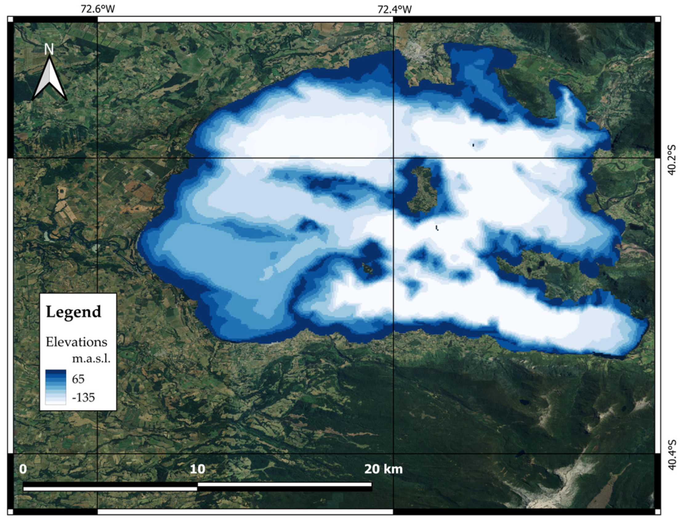
2.1. Site Description

Lake Ranco, one of the largest lakes in Chile, is located at 40°13′ south latitude and 72°23′ west longitude in the Los Rios Region. It has a surface area of approximately 442 km² and a perimeter of approximately 154 km. Lake Ranco’s environment is mountainous and rugged. The lake has several islands, of which Huapi Island is one of the largest and most important. These islands contribute to the beauty of the landscape and offer possibilities for exploration and discovery. The region features a humid temperate climate with Mediterranean characteristics [37]. The average precipitation is 2000 mm/year, and the average annual temperature fluctuates between 6 and 9 °C, with maxima in January (20 °C) and minima in July (2 °C), according to the Chilean Meteorological Directorate (DMC, http://www.meteochile.cl/, accessed on 1 March 2024). From the production point of view, there are four relevant activities in the unit’s economic productive matrix: the agricultural system, tourism, forestry, and the hydrobiological system [38,39]. The basin’s land use is distinguished by a substantial portion covered by native forests, which account for 51% of its total surface area. Water bodies constitute another significant category, occupying 13% of the basin, followed by grasslands at 10%. Forest plantations, on the other hand, represent the most minor portion, comprising only 0.6% of the total surface area [39]. The location of Lake Ranco in Chile, Los Ríos Region, and the location of its basin are presented in Figure 1. The bathymetry of Lake Ranco is presented in Figure 2, and its morphological information is presented in

Table 1. Morphometric parameters of Lake Ranco and its basin.

Parameters	Unit	Ranco
Latitude	°S	40°13′
Longitude	°W	72°23′
Altitude	m.a.s.l.	69
Perimeter	km	154.6
Max width	km	30.43
Median width	km	1.59
Superficial area (A)	km2	442.62
Max depth	m	199
Median depth	m	122.13
Volume	km3	54.06
Watershed area (ad)	km2	3498
Ad/a		3.7
Renovation time	years	5

. Additionally, the variation curves of lake area and volume are shown in Figure 3.

2.2. Meteorological Data

In the present study, a 5-year time series (2017–2023) of lake-level data based on information from the Dirección General de Aguas (DGA) database (accessed on 23 December 2023) was considered. The lake-level information was analyzed with respect to hydrometeorological data from the same time, such as precipitation, temperature, relative humidity, potential evapotranspiration, and the El Niño−Southern Oscillation (ENSO 3.4) and Pacific Decadal Oscillation (PDO) anomalies over the study period.

Five meteorological stations controlled by the DGA were used to estimate precipitation in the basin. The details of the stations are shown in

Table 2. Information from meteorological stations controlled by the Dirección General de Aguas in the Lake Ranco basin.

Rain Gauge Station		Latitude	Longitude	Period of Availability
C1	El Llolly	−40.067°	−72.616°	November 1994–October 2020
C2	Lago Ranco	−40.317°	−72.469°	January 1958–January 2021
C3	Caunahue	−40.159°	−72.252°	January 2012–October 2020
C4	Río Calcurrupe en Desembocadura	−40.231°	−72.260°	January 2013–August 2020
C5	Lago Maihue	−40.218°	−72.146°	January 1981–October 2020

, and their spatial location can be seen in Figure 1.

The methodology for processing meteorological information from the Lake Ranco basin is detailed below.

• Fill gaps in precipitation data through a regional analysis using linear regression, as detailed in [40,41].
• For the estimation of precipitation over the Lake Ranco basin, the inverse-of-distance (IDW) method was used [42], providing a weighting associated with the distance of each station to the centroid of the lake basin (blue point in Figure 1c). Additionally, meteorological data from dates until December 2023 were supplemented with information from the CHIRPS [43] and the In-Line Hydrometric System of the DGA.

We employed a diverse array of data sources to comprehensively understand the basin’s climate. Temperature, relative humidity, and potential evapotranspiration of the basin were obtained from the CAMELS-CL database [44] and the In-Line Hydrometric System of the DGA, with daily data covering the period from January 1979 to December 2023. Potential evapotranspiration was calculated as Hargreaves and Samani [45] proposed, ensuring a thorough and complete analysis.

2.3. Radar Altimetry Data

Four satellite missions, ERS-2, ENVISAT, SARAL, and Sentinel-3A, were used for this analysis. These missions were selected because their orbit passes over Lake Ranco. During the 1990s, the European Space Agency (ESA) initiated its ERS program by launching two satellites: ERS-1, in July 1991, and ERS-2, in April 1995. ERS-1 functioned effectively until June 1996, while ERS-2 continued operations until November 2003. Throughout its operation, ENVISAT delivered continuous observations of the oceans, land, and cryosphere up to latitudes of ±81.5°N on a sun-synchronous orbit with a repeat cycle of 35 days. The radar altimeter (RA) on the ERS satellites operated in Ku-band with a frequency of 13.8 GHz [46]. To extend the dataset and maintain continuity with the subsequent ENVISAT mission, data from ERS-2, as part of the ESA’s Reaper project [47], were utilized up to July 2003. Also, the European Space Agency (ESA) successfully launched Envisat from the European Spaceport located in French Guiana on 1 March 2002, marking the beginning of a mission that concluded on 8 April 2012. ENVISAT was placed on the same orbit as ERS-1 and ERS-2. It was equipped with the Advanced Radar Altimeter 2 (RA-2), which utilized a dual-frequency radar signal (Ku-band at 13.575 GHz and S-band at 3.2 GHz). [48]. In addition, SARAL, or Satellite with Argos and ALtiKa, was launched on 25 February 2013 and was operating in its nominal orbit until July 2016 [28]. The mission followed the same 35-day repeat orbit as ERS-1 and ERS-2, and ENVISAT at ~800 km of altitude with an inclination of 98.54° [36]. The French/Indian satellite mission mainly involved the AltiKa Ka-band altimeter system operating for Precise Orbit Determination (POD); the spacecraft carried a Laser Retroreflector Array (LRA) and the DORIS DGXX receiver to meet the radial-orbit-altimetry mission requirement of 3 cm and potentially to meet the 2-cm goal [49]. Finally, the Sentinel-3A satellite was launched on 16 February 2016. It is in an orbit at a 814.5 km altitude and a heliosynchronous orbit of 98.65° inclination with a repetition cycle of 27 days and an equatorial separation of about 105 km (Sentinel-3A and Sentinel-3B are in the same orbit, with a phase difference of 180°) [50], composed of SRAL (SAR Radar ALtimeter), a dual-frequency SAR altimeter (Ku-band at 13.575 GHz and C-band at 5.41 GHz), and a dual-frequency SAR at 5.41 GHz [51].

ENVISAT, SARAL, and Sentinel-3A data came from the Geophysical Data Records (GDR) made available by CNES/ISRO and ESA, while the ERS-2 data came from the reprocessing dedicated to hydrology conducted by CTOH [52].

The Sentinel-3A data were used to evaluate the performance of the altimetry data through comparisons with in situ water levels, while the ERS-2, ENVISAT, and SARAL data were used to extend the time series of the Lake Ranco level for the period 1995–2017 to complement the Sentinel-3A data. The data obtained from these missions will be calibrated using Sentinel-3A results.

2.4. Retrieving Altimetry-Based Water Levels Using AlTiS Software

AlTiS (Altimetry Time Series) is an advanced radar-altimetry data-processing and visualization software that is designed to enable thorough examinations of minute water bodies [33] and that replaced the previous Multimission Altimetry Processing Software (v2.2.9-0-gf5938ab) [52]. Its main objective is to derive a time series of water levels from radar-altimetry measurements. To help the user obtain accurate altimetry-based time series of water levels, it allows the visualization and processing (including the generation of time series) of auxiliary information, such as range corrections, backscatter coefficients from the radar altimeter, and brightness temperatures from the microwave radiometer [20]. AlTiS has been successfully used to estimate lake levels in Vietnam [53], Ivory Coast (Lake Buyo) [54], Cambodia (Lake Tonle Sap Lake) [55], and Sweden [56], among others. AlTiS is a Python-based Graphical User Interface (GUI) using the wxWidgets cross-platform library, which makes it possible to [33]

• Read radar-altimetry data from ERS-2, ENVISAT, JASON-1/2/3, SARAL, and the Sentinel-3A and 3B radar-altimetry missions.
• Display the different variables contained in the Geophysical Data Records (GDR) of each mission, including the height of the satellite in its orbit (H); the radar range (R0); the different corrections applied to R0 (ΣR); h, which is automatically computed when reading the data as h = H − R0 – ΣR; as well as several other variables, such as the backscattering coefficients and the pulse peakiness at the different microwave frequencies; the brightness temperatures at the different frequencies measured by the radiometer onboard the satellite platform; and the normalized index defined by CTOH to help with the statistical analysis, with the Landsat True-Color image supplied by the Global Imagery Browse Services (GIBS from NASA’s Earth observations) as background.
• Manually select the valid data/remove the invalid data, contouring them using the mouse.
• Generate the time series of water levels, computing the median and mean values and the associated median absolute deviation and standard deviation for each cycle. Note that the different altimeter tracks were processed individually. In this study, median values and associated median absolute deviations computed each cycle were used to minimize the potential impact of residual outliers on a small number of observations due to the moderate width of the lakes under the altimeter tracks.

2.5. Validation of Lake Water Levels Based on Altimetry

Validation of the AlTiS results was performed quantitatively using several objective functions, which are described below.

2.5.1. Root Mean Square Error (RMSE)

RMSE can be considered a multipurpose criterion centered on simulated data [13]. This function is focused on high streamflow error [57,58] and can be calculated using Equation (1), as follows:

$$\mathrm{RMSE}=\sqrt{\frac{{{\displaystyle \sum }}_{\mathrm{i}=1}^{\mathrm{n}}{\left({\mathrm{WL}}_{\mathrm{altimetry}}-{\mathrm{WL}}_{\mathrm{in} \mathrm{situ}}\right)}^2}{\mathrm{n}}}$$

(1)

where $\mathrm{W}{\mathrm{L}}_{\mathrm{a}\mathrm{l}\mathrm{t}\mathrm{i}\mathrm{m}\mathrm{e}\mathrm{t}\mathrm{r}\mathrm{y}}$ and $\mathrm{W}{\mathrm{L}}_{\mathrm{i}\mathrm{n} \mathrm{s}\mathrm{i}\mathrm{t}\mathrm{u}}$ are the simulated and observed water levels in Lake Ranco and n is the length of the time series. RMSE measures differences between estimated and observed water levels and has the units of measurement of the analyzed data (m). A RMSE equal to zero indicates a perfect fit between the estimated and observed series, while the greater the RMSE value, the worse the fit between the estimated and observed series. If the RMSE values are less than half of the standard deviation of the observed data, it can be considered low and indicate good model prediction [59].

2.5.2. Kling−Gupta Efficiency (KGE)

The KGE index is the result of the decomposition of the Nash−Sutcliffe efficiency (NSE) and is focused on equitably evaluating the correlation, deviation, and variability of the estimated data [60]. It can be calculated with Equation (2), as follows:

$$\mathrm{KGE}=1-\sqrt{\left(\mathrm{r}-1\right)+\left(\mathsf{\alpha }-1\right)+\left(\mathsf{\beta }-1\right)}$$

(2)

where r is the coefficient of linear correlation between the estimated and the observed data, $\mathsf{\alpha }$ is a measure of the variability of the data values (equal to the standard deviation of the estimated data over the standard deviation of the observed data), and $\mathsf{\beta }$ is the average of the estimated data over the average of the observed data. In the literature, the threshold value for a model to be considered suitable is KGE ≥ 0.6 [61].

2.5.3. Index of Agreement

The agreement index serves as a standardized metric evaluating the accuracy of data estimation. Calculated as the ratio between the mean square error and the potential error, it offers insight into the fidelity of a model’s predictions. Ranging from 0 to 1, where 1 signifies an optimal match between predicted and actual values and 0 indicates no discernible correspondence, this index provides a concise measure of the model’s performance [62,63]. It can be calculated with Equation (3), as follows:

$$\mathrm{d}=1-\frac{{{\displaystyle \sum }}_{\mathrm{i}=1}^{\mathrm{n}}{\left({\mathrm{WL}}_{\mathrm{in} \mathrm{situ}}-{\mathrm{WL}}_{\mathrm{altimetry}}\right)}^2}{{{\displaystyle \sum }}_{\mathrm{i}=1}^{\mathrm{n}}({\left|{\mathrm{WL}}_{\mathrm{atimetry}}-\overline{{\mathrm{WL}}_{\mathrm{in} \mathrm{situ}}}+\left|{\mathrm{WL}}_{\mathrm{in} \mathrm{situ}}-\overline{{\mathrm{WL}}_{\mathrm{in} \mathrm{situ}}}\right|)\right|}^2}$$

(3)

2.5.4. Coefficient of Determination (R²)

The coefficient of determination describes the degree of collinearity between observed and estimated information. This value ranges between 0 and 1. A value of 1 indicates a smaller error in the variance. Generally, a value of 0.5 can be considered acceptable [64]. It can be calculated with Equation (4), as follows:

$${\mathrm{R}}^2=\frac{{\left[{{\displaystyle \sum }}_{\mathrm{i}=1}^{\mathrm{n}}\left({\mathrm{WL}}_{\mathrm{altimetry}}-\overline{{\mathrm{WL}}_{\mathrm{in} \mathrm{situ}}}\right)·\left({\mathrm{WL}}_{\mathrm{in} \mathrm{situ}}-\overline{{\mathrm{WL}}_{\mathrm{altimetry}}}\right)\right]}^2}{{{\displaystyle \sum }}_{\mathrm{i}=1}^{\mathrm{n}}{\left({\mathrm{WL}}_{\mathrm{altimetry}}-\overline{{\mathrm{WL}}_{\mathrm{altimetry}}}\right)}^2·{{\displaystyle \sum }}_{\mathrm{i}=1}^{\mathrm{n}}{\left({\mathrm{WL}}_{\mathrm{in} \mathrm{situ}}-\overline{{\mathrm{WL}}_{\mathrm{in} \mathrm{situ}}}\right)}^2}$$

(4)

2.6. Calculation of the Surface Area and Volume of Lake Ranco

After the Sentinel 3A data had been validated, the surface area and volume of Lake Ranco were computed. To achieve this, specific curves correlating to these variables were generated, as depicted in Figure 3. These curves serve as a tool for accurately determining the lake’s surface area and volume based on its water level at any given time. These curves were constructed using the topo-bathymetric information of Lake Ranco, as comprehensively presented in Figure 2. This methodological approach ensures precision in calculations and understanding of the lake’s dynamics by providing a clear visual representation of how its physical characteristics fluctuate with changes in water level.

2.7. Climate Indices

2.7.1. El Niño 3.4 Sea Surface Temperature Index

ENSO is a natural cycle caused by fluctuations in the sea surface temperature (SST) originating from the strengthening and weakening of trade winds [65]. The ENSO phenomenon consists of two phases: El Niño (i.e., higher rainfall and lower winds), which is when the SST increases and which is considered the warm phase, and La Niña (i.e., lower rainfall and increased winds), which is when the SST decreases and which is considered the cold phase [66]. El Niño Southern Oscillation (ENSO) oceanic indices are defined using the SST anomaly averaged over the east-central equatorial region. The El Niño 3.4 SST Index is computed over a region located in the eastern Pacific, between longitude 120° W and 170° W and latitude 5° N and 5° S [18,67,68]. It is available on a monthly time step starting from January 1950 at the following address: https://www.ncei.noaa.gov/access/monitoring/enso/sst (acceded on 20 March 2024). According to Montecinos and Aceituno [69], the El Niño 3.4 index represents the effects of the ENSO phenomena in Chile, especially the changes in precipitation.

2.7.2. Pacific Decadal Oscillation Index

The Pacific Decadal Oscillation (PDO) Index is defined as the principal component of monthly SST variability in the North Pacific poleward of 20°N [18]. Extreme PDO patterns are marked by widespread variations in the Pacific Basin and North American climates. The extreme phases of the PDO have been classified as being warm or cool, as defined by the ocean temperature in the northeast and tropical Pacific Ocean [70,71]. It is available on a monthly time step starting from January 1854 at the following address: https://www.ncei.noaa.gov/access/monitoring/pdo/ (acceded on 20 March 2024).

3. Results

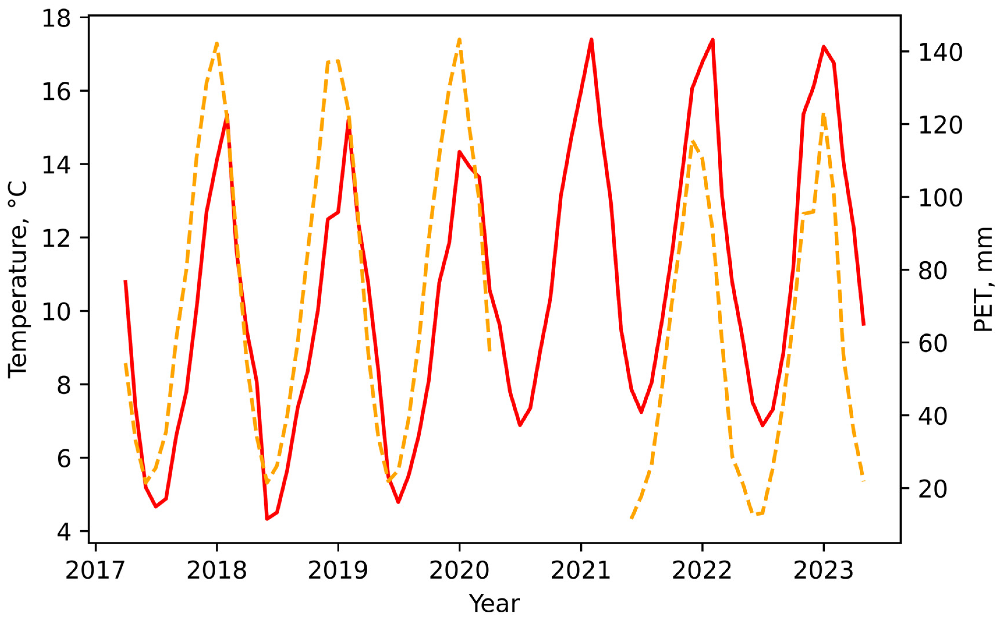
3.1. Meteorological Behavior during the Study Period

The results of the filling and interpolation of precipitation data within the Lake Ranco basin can be seen in Figure 4 for the periods (a) 1995–2023 and (b) 2017–2023 and can also be seen in

Table 3. Accumulated precipitation [mm] in the Lake Ranco basin. Information was obtained from the DGA, CAMELS-CL, and CHIRPS databases.

Year	Accumulated Precipitation, mm	Standard Deviation, mm
1995	1904	45.57
1996	1627	40.14
1997	2439	39.94
1998	1184	42.02
1999	1801	45.09
2000	2232	39.78
2001	1887	42.48
2002	2446	42.85
2003	1956	38.05
2004	1982	43.70
2005	2135	43.02
2006	2287	41.02
2007	1610	42.16
2008	1912	48.39
2009	2020	41.77
2010	1738	39.52
2011	1789	45.23
2012	2081	42.26
2013	1364	46.96
2014	1570	41.46
2015	1895	44.92
2016	1222	44.42
2017	1675	42.44
2018	1836	43.36
2019	1601	42.56
2020	1626	36.30
2021	1644	39.61
2022	1751	35.86
2023	1367	38.13

. In all cases, Chile’s hydrological year, which varies between April and March, was used. In addition, the relative humidity data for the area under study were added. There is a period without information due to the lack of current stations that would make it possible to obtain these data. When the entire period (1995–2023) shown in Figure 4a and Table 3 was analyzed, it was found that the maximum rainfall in the area under study occurred in 2006, at 2287 mm, while the minimum values occurred in 1998 with 1184 mm. Additionally, it was possible to observe a decrease in precipitation starting in 2010 and then starting to increase towards the last period, as shown in Figure 4a and Table 3. If we analyze the averages for the periods 1995–2009 and 2010–2023, we obtain annual precipitation values of 1962 ± 332 and 1654 ± 227 mm, respectively, indicating a decrease in the annual precipitation over the study area by 10%. Nonetheless, when analyzing the period under study (Figure 4b), it is possible to observe a 9.37% increase in accumulated precipitation.

In addition, Figure 5 shows the variations in temperature and potential evapotranspiration over Lake Ranco. It is possible to note that there is a break in the information between 2021 and 2022. This lack of data is associated with periods of maintenance or damage to the monitoring station of the Dirección General de Aguas. From this point, there was a slight decrease in temperature over the same period (1.14%), which influenced the evapotranspiration rate in the region. The increase in precipitation in the last period (2020–2023), together with the decrease in potential evapotranspiration, could promote an increase in the levels of Lake Ranco.

3.2. Altimetry-Based Time Series of Water Levels

The series of water levels over 2017–2023 obtained from the DGA In-Line Hydrometeorological System and derived from Sentinel-3A altimetry measurements are shown in Figure 6. They both exhibit a well-marked seasonal cycle with an amplitude between 1.34 and 1.68 m, strong interannual variability, and an increasing trend over 2017–2023 (red line).

A comparison of water-level data from different sources yielded an RMSE of 0.04 m, an index of agreement of 0.99, an R² of 0.99, and a coefficient KGE = 0.90, showing the very good agreement between the observed values from the DGA database and altimetry derived from Sentinel-3A estimates. This is why it is possible to use altimetry-based water levels to replace the missing data for Lake Ranco and estimate the variation in the volume and surface area of the water body. This information, combined with the data in Figure 3, is shown in Figure 7, as mentioned in point 2.6 of the methodology.

The maximum values of surface area and lake volume coincide on 18 July 2020, with values of 537.375 km² and 54.3441 km³, respectively. Additionally, the minimum values for both variables coincide on 20 March 2019, with surface area and volume values of 526.944 km² and 54.3441 km³, respectively. Ranges of surface height and volume of 10.43 km² and 0.0434 km³, respectively, were obtained for the period under study. The maximum values coincide with the 2020 winter period, when 62% of the year’s precipitation had already been recorded. Additionally, the minimum values occurred in March 2019, at the end of the hydrological year in Chile, where the lowest precipitation, water level, and flow values in various continental water bodies are expected. By this point, only 6% of the annual precipitation had been recorded, a point that aligns with the high standard deviation of the year’s precipitation data, as shown in Table 3 (standard deviation of 42.56 mm). This suggests that precipitation was concentrated in specific periods of the year, primarily during winter. Finally, the validated information on the level of Lake Ranco was complemented by data from ERS-2, ENVISAT, and SARAL from 1995–2017, as shown in Figure 8. It should be mentioned that there are no DGA records to validate this information. However, the data were adjusted according to the difference observed between the data from the DGA and the Sentinel-3A mission. This adjustment corresponds to the less than 1% decrease in the value recorded by the satellite. Likewise, Figure 9a,b shows the variation in the surface area and volume of Lake Ranco in the 1995–2023 period.

In Figure 9, both lake surface and volume move within a narrow range of variation (0.014 km³ and 4.96 km² for the volume and area, respectively). It is possible to note the relationship between the variation in area and volume in the area under study. However, since 2010, there has been a decrease and greater variability in the values, which may be influenced primarily by changes in precipitation in the area. In addition, Figure 10a,b shows the ENSO 3.4 anomalies and the variation in the PDO index from 1995 to 2023, respectively. Also, Figure 10c,d shows the annual anomalies in the area and volume of Lake Ranco between 1995 and 2023, respectively. The anomaly range of lake volume was 0.0139 km³ in 2015 (17.5% of the 1995–2023 average annual lake volume variations) and −0.0151 km³ in 2016 (16.1% of the 1995–2023 average annual lake volume variations), and the anomaly range of surface lake area was 4.031 km² (15.2% of the 1995–2023 average lake surface) in 2015 and −3.792 km² in 2016 (16.2% of the 1995–2023 average lake surface).

4. Discussion

Understanding fluctuations in lake levels is vitally important for unraveling the complexities of river flow dynamics and oscillations in water-reservoir volumes [4]. Leveraging radar satellites, which provide continuous time-series data, is critical to gaining deep insights into water-level dynamics [72].

To determine the accuracy of altimetry-based water levels, we compared them to the data in the DGA database. Our comparison exceeds the minimum threshold values set for the root mean square error (RMSE), index of agreement, correlation coefficient (R), and Kling−Gupta efficiency (KGE) proposed by [59,62,64] and [60], with values of 0.04 m, 0.99, 0.99, and 0.90, respectively, as illustrated in Figure 6, which proves the good fit of the lake levels with the altimetry data. These good results are in keeping with the results of previous studies comparing altimetry-based water levels within situ measurements (e.g., [16,19,33,73]). The good agreement between in situ and the use of altimetry-based water levels made it possible to use the satellite data to estimate the volume and surface area of Lake Ranco by merging the level data with the bathymetric information (Figure 2) over 1995–2023, as illustrated in Figure 9. The area and volume show synchronized behavior, reflecting the general trend observed in lake levels during the study period (Figure 7). To improve our understanding, the Sentinel-3A data used to estimate the level of Lake Ranco were complemented by ERS-2, ENVISAT, and SARAL data covering the period 1995–2017. One of the main advantages of this work is the possibility of complementing existing lake-level time series or of being able to have records in areas where there are no monitoring networks. It is proposed to study other lake bodies in Chile to validate the method in different climatic zones.

Our analysis reveals a notable increase in cumulative precipitation (9.37%) across the study area from 2017 to 2023, as illustrated in Figure 4b and detailed in Table 3. At the same time, there is discernible evidence indicating a slight decrease in temperature over the same period (1.14%), which influences evapotranspiration rates in the region, as shown in Figure 5. Furthermore, these fluctuations align with shifts in precipitation patterns observed in Lake Ranco (refer to Figure 4a,b, and Table 3). Notably, precipitation levels exhibit a steady trend from 1995 to 2010, which was followed by a decline thereafter, with a marginal uptick noted in the latest period. The behavior of the lake level in the period 1995–2023 shows similarities with the changes in precipitation in the area during the same period (Figure 4a), with a relatively constant level until 2010, when the level decreased. The lake level has shown a pronounced decrease since 2010, and this decrease was maintained until 2019, when the lake began to increase its level again, concurrent with the increase in precipitation (Figure 4a) and the decrease with evapotranspiration (Figure 5). In addition, it is imperative to have a greater amount of temperature data in order to be able to perform analyses such as the ones proposed in Noori et al. [15,74].

The pronounced decline in precipitation across central Chile, exacerbated by a series of consecutive dry years since 2010 (Figure 4a), has been notable, with annual precipitation deficits ranging from 25% to 45% [75]. Furthermore, according to NOAA records, the years 2010 to 2012 witnessed some of the most intense ENSO (La Niña) events in recent history, enhanced by a cold phase of the PDO (see Figure 10a,b). This decrease persisted until 2016, when an ENSO (El Niño) event occurred, leading to increased rainfall and river overflows in south-central Chile. The El Niño episode between 2015 and 2016 is ranked as one of the strongest since 1950 [76] and coincides with the warm phase of the PDO. This could elucidate the observed decrease in the level of Lake Ranco, as depicted in Figure 8. It is possible to note a correlation between the cold phases of ENSO 3.4 (i.e., La Ñiña) and the PDO index, leading to drier years. Moreover, Figure 10a illustrates cold-phase ENSO and a PDO (i.e., La Niña) phenomena before 2019, potentially contributing to the observed decrease in lake area and volume as discussed earlier. Conversely, a warm-phase ENSO event (i.e., El Niño) is depicted during 2020, likely associated with increased precipitation in the area and resulting in the peak values of volume and area in Lake Ranco. Henley [77] determined that a positive PDO leads to higher precipitation to the south and decreased precipitation to the north. Larger anomalies occur when the ENSO index and PDO index exhibit large deviations and are in phase [18]. An increase in the effects can be observed when the warm or cold phases of ENSO 3.4 and the PDO index coincide. Sagarika et al. [66] determined that ENSO phenomena are an important forcing factor in the annual flow variations in the Andean basins, while, to a lesser extent, the PDO also affects these variations. Such meteorological dynamics probably contributed to fluctuations in Lake Ranco’s levels during the specified period. A decrease in precipitation has been observed since 2010, coinciding with ENSO phenomena in the cold phase (i.e., La Niña), which could explain the change in the level, volume, and area of the lake under study. This is consistent with Chile’s mega-drought, as detailed by Garreaud et al. [75,78] and Boisier et al., [79]. When comparing the ENSO phenomena (Figure 10a) with the area and volume anomalies of Lake Ranco (Figure 10c,d, respectively), it is possible to note that the warm ENSO pass coincides with the positive area and volume anomalies, while the cold ENSO phases coincide with negative anomalies. It is worth mentioning that the anomalies increase when the ENSO and PDO phenomena are in phase (i.e., their warm or cold phases coincide).

The methodology employed in this study can be extrapolated to assess the status of water levels and volumes in all Chilean aquatic ecosystems intersecting the orbits of satellites with onboard altimeters. This approach, possibly combined with lake surface-extent monitoring from space (see [18]), offers a promising avenue for comprehensive monitoring and management of water resources throughout Chile.

5. Conclusions

The use of altimetry information from different missions is crucial to understanding lake-level variations and has been tested in several studies over time. In this context, Sentinel-3A data show a high level of agreement with data from Lake Ranco in Chile according to the target functions selected for the development of this work (KGE = 0.99, RMSE = 0.04, and Index of agreement = 0.99). Due to the good fit shown by the comparison of the levels of Lake Ranco with the data of the Dirección General de Aguas, it was possible to estimate the variation in the area and volume of the lake for the period 1995–2023, considering data from the ERS-2, ENVISAT, SARAL, and Sentinel-3A missions. Variations in lake level, area, and volume are related to the variation in precipitation over the study area. This variable shows a decrease of 10% between the mean values of the 1995–2010 and 2010–2023 periods. However, this variable shows an increase of 9.37% in the last period. In addition, it is possible to observe a decrease in temperature and potential evapotranspiration in the period 2017–2023, which could have contributed to the behavior of the level, area, and volume of Lake Ranco. Moreover, the area and volume of Lake Ranco were affected by the ENSO and PDO climatic phenomena. As an example, the ENSO (i.e., El Niño) phenomenon of the 2015–2016 period, cataloged as one of the most intense in recent times, coincided with the warm phase of the PDO, which caused an increase in precipitation in the lake under study and positive anomalies for area and volume. Consequently, when the ENSO and PDO coincided in their cold phase (e.g., period 2010–2012), a decrease in the levels of Lake Ranco and an increase in the area and volume anomaly were observed.

Finally, it is possible to use altimetry to estimate the level, volume, and surface area of this lake. With this information, it is possible to have greater control over the water rights of each body of water in Chile in the event of drought or better control of water quality after flooding processes. In addition, it would allow entities associated with water resources to evaluate various bodies of water that currently have a low number of hydrometric records. However, it is essential to have in situ information to validate the method. This can be complex in Chile, since lake-level records are usually current, which makes it difficult to validate past missions (as in the case of ERS-2 and ENVISAT). Despite this, this methodology is useful for research on water resources and the implications of various meteorological events. In addition, wind effects in the study area are not considered, which could cause alterations in the study area and changes in meteorological variables. Additionally, multi-satellite studies that include current altimetric missions, highlighting the use of SWOT, are proposeds.

References

1. Magee, M.R.; Hein, C.L.; Walsh, J.R.; Shannon, P.D.; Vander Zanden, M.J.; Campbell, T.B.; Hansen, G.J.A.; Hauxwell, J.; LaLiberte, G.D.; Parks, T.P.; et al. Scientific Advances and Adaptation Strategies for Wisconsin Lakes Facing Climate Change. Lake Reserv. Manag. 2019, 35, 364–381. [Google Scholar] [CrossRef]
2. Mohammed, A.S.; Gafa, D.W.; Atanga, R.A. Sustainable Development: Conceptual and Theoretical Insights in the Global South. In Sustainable and Responsible Investment in Developing Markets; Abor, J., Ed.; Elgar Publishing: Cheltenham, UK, 2023; pp. 141–157. [Google Scholar]
3. Crétaux, J.F.; Abarca-del-Río, R.; Bergé-Nguyen, M.; Arsen, A.; Drolon, V.; Clos, G.; Maisongrande, P. Lake Volume Monitoring from Space. Surv. Geophys. 2016, 37, 269–305. [Google Scholar] [CrossRef]
4. Jiang, L.; Schneider, R.; Andersen, O.B.; Bauer-Gottwein, P. CryoSat-2 Altimetry Applications over Rivers and Lakes. Water 2017, 9, 211. [Google Scholar] [CrossRef]
5. Oki, T.; Entekhabi, D.; Harrold, T. The Global Water Cycle. Global Energy and Water Cycles. Energy Water Cycles 1999, 1999, 10–29. [Google Scholar]
6. Yao, F.; Livneh, B.; Rajagopalan, B.; Wang, J.; Crétaux, J.-F.; Wada, Y.; Berge-Nguyen, M. Satellites Reveal. Widespread Decline in Global Lake Water Storage. Science 2023, 380, 6646. [Google Scholar] [CrossRef] [PubMed]
7. Cooley, S.W.; Ryan, J.C.; Smith, L.C. Human Alteration of Global Surface Water Storage Variability. Nature 2021, 591, 78–81. [Google Scholar] [CrossRef] [PubMed]
8. Bovermann, Z.E.; Fallah-Mehdipour, E.; Arumí, J.L.; Dietrich, J. The Chilean Laja Lake: Multi-Objective Analysis of Conflicting Water Demands and the Added Value of Optimization Strategies. Aqua Water Infrastruct. Ecosyst. Soc. 2024, 73, 369–379. [Google Scholar] [CrossRef]
9. Barría, P.; Chadwick, C.; Ocampo-Melgar, A.; Galleguillos, M.; Garreaud, R.; Díaz-Vasconcellos, R.; Poblete, D.; Rubio-Álvarez, E.; Poblete-Caballero, D.; Cramer, W. Water Management or Megadrought: What Caused the Chilean Aculeo Lake Drying? Reg. Environ. Chang. 2021, 21, 19. [Google Scholar] [CrossRef]
10. Schilling, J.; Hertig, E.; Tramblay, Y.; Scheffran, J. Climate Change Vulnerability, Water Resources and Social Implications in North Africa. Reg. Environ. Chang. 2020, 20, 15. [Google Scholar] [CrossRef]
11. Prakash, S. Impact of climate change on aquatic ecosystem and its biodiversity: An overview. Int. J. Biol. Innov. 2021, 3, 2. [Google Scholar] [CrossRef]
12. Noori, R.; Woolway, R.I.; Saari, M.; Pulkkanen, M.; Kløve, B. Six Decades of Thermal Change in a Pristine Lake Situated North of the Arctic Circle. Water Resour. Res. 2022, 58, e2021WR031543. [Google Scholar] [CrossRef]
13. Medina, Y.; Muñoz, E. Estimation of Annual Maximum and Minimum Flow Trends in a Data-Scarce Basin. Case Study of the Allipen River Watershed, Chile. Water 2020, 12, 162. [Google Scholar] [CrossRef]
14. Kreibich, H.; Van Loon, A.F.; Schröter, K.; Ward, P.J.; Mazzoleni, M.; Sairam, N.; Abeshu, G.W.; Agafonova, S.; AghaKouchak, A.; Aksoy, H.; et al. The Challenge of Unprecedented Floods and Droughts in Risk Management. Nature 2022, 608, 80–86. [Google Scholar] [CrossRef] [PubMed]
15. Noori, R.; Woolway, R.I.; Jun, C.; Bateni, S.M.; Naderian, D.; Partani, S.; Maghrebi, M.; Pulkkanen, M. Multi-Decadal Change in Summer Mean Water Temperature in Lake Konnevesi, Finland (1984–2021). Ecol. Inform. 2023, 78, 102331. [Google Scholar] [CrossRef]
16. Shu, S.; Liu, H.; Beck, R.A.; Frappart, F.; Korhonen, J.; Lan, M.; Xu, M.; Yang, B.; Huang, Y. Evaluation of Historic and Operational Satellite Radar Altimetry Missions for Constructing Consistent Long-Term Lake Water Level Records. Hydrol. Earth Syst. Sci. 2021, 25, 1643–1670. [Google Scholar] [CrossRef]
17. Verpoorter, C.; Kutser, T.; Seekell, D.A.; Tranvik, L.J. A Global Inventory of Lakes Based on High-Resolution Satellite Imagery. Geophys. Res. Lett. 2014, 41, 6396–6402. [Google Scholar] [CrossRef]
18. Frappart, F.; Biancamaria, S.; Normandin, C.; Blarel, F.; Bourrel, L.; Aumont, M.; Azemar, P.; Vu, P.L.; Le Toan, T.; Lubac, B.; et al. Influence of Recent Climatic Events on the Surface Water Storage of the Tonle Sap Lake. Sci. Total Environ. 2018, 636, 1520–1533. [Google Scholar] [CrossRef] [PubMed]
19. Birkett, C.M.; Beckley, B. Investigating the Performance of the Jason-2/OSTM Radar Altimeter over Lakes and Reservoirs. Mar. Geod. 2010, 33, 204–238. [Google Scholar] [CrossRef]
20. Frappart, F.; Blarel, F.; Papa, F.; Prigent, C.; Mougin, E.; Paillou, P.; Baup, F.; Zeiger, P.; Salameh, E.; Darrozes, J.; et al. Backscattering Signatures at Ka, Ku, C and S Bands from Low Resolution Radar Altimetry over Land. Adv. Space Res. 2021, 68, 989–1012. [Google Scholar] [CrossRef]
21. Nielsen, K.; Zakharova, E.; Tarpanelli, A.; Andersen, O.B.; Benveniste, J. River Levels from Multi Mission Altimetry, a Statistical Approach. Remote Sens. Environ. 2022, 270, 112876. [Google Scholar] [CrossRef]
22. Cretaux, J.F.; Calmant, S.; Papa, F.; Frappart, F.; Paris, A.; Berge-Nguyen, M. Inland Surface Waters Quantity Monitored from Remote Sensing. Surv. Geophys. 2023, 44, 1519–1552. [Google Scholar] [CrossRef]
23. Hossain, F.; Siddique-E-Akbor, A.H.; Mazumder, L.C.; Shahnewaz, S.M.; Biancamaria, S.; Lee, H.; Shum, C.K. Proof of Concept of an Altimeter-Based River Forecasting System for Transboundary Flow Inside Bangladesh. IEEE J. Sel. Top. Appl. Earth Obs. Remote Sens. 2014, 7, 587–601. [Google Scholar] [CrossRef]
24. Da Silva, J.S.; Calmant, S.; Seyler, F.; Moreira, D.M.; Oliveira, D.; Monteiro, A. Radar Altimetry Aids Managing Gauge Networks. Water Resour. Manag. 2014, 28, 587–603. [Google Scholar] [CrossRef]
25. Raney, R.K. The Delay/Doppler Radar Altimeter. IEEE Trans. Geosci. Remote Sens. 1998, 36, 1578–1588. [Google Scholar] [CrossRef]
26. Jensen, J.R. Angle Measurement with a Phase Monopulse Radar Altimeter. IEEE Trans. Antennas Propag. 1999, 47, 715–724. [Google Scholar] [CrossRef]
27. Fjørtoft, R.; Gaudin, J.-M.; Pourthié, N.; Lalaurie, J.-C.; Mallet, A.; Nouvel, J.-F.; Martinot-Lagarde, J.; Oriot, H.; Borderies, P.; Ruiz, C.; et al. KaRIn on SWOT: Characteristics of Near-Nadir Ka-Band Interferometric SAR Imagery. IEEE Trans. Geosci. Remote Sens. 2014, 52, 2172–2185. [Google Scholar] [CrossRef]
28. Bonnefond, P.; Verron, J.; Aublanc, J.; Babu, K.N.; Bergé-Nguyen, M.; Cancet, M.; Chaudhary, A.; Crétaux, J.F.; Frappart, F.; Haines, B.J.; et al. The Benefits of the Ka-Band as Evidenced from the SARAL/AltiKa Altimetric Mission: Quality Assessment and Unique Characteristics of AltiKa Data. Remote Sens. 2018, 10, 83. [Google Scholar] [CrossRef]
29. Biancamaria, S.; Frappart, F.; Leleu, A.S.; Marieu, V.; Blumstein, D.; Desjonquères, J.D.; Boy, F.; Sottolichio, A.; Valle-Levinson, A. Satellite Radar Altimetry Water Elevations Performance over a 200 m Wide River: Evaluation over the Garonne River. Adv. Space Res. 2017, 59, 128–146. [Google Scholar] [CrossRef]
30. Biancamaria, S.; Schaedele, T.; Blumstein, D.; Frappart, F.; Boy, F.; Desjonquères, J.D.; Pottier, C.; Blarel, F.; Niño, F. Validation of Jason-3 Tracking Modes over French Rivers. Remote Sens. Environ. 2018, 209, 77–89. [Google Scholar] [CrossRef]
31. Normandin, C.; Frappart, F.; Diepkilé, A.T.; Marieu, V.; Mougin, E.; Blarel, F.; Lubac, B.; Braquet, N.; Ba, A. Evolution of the Performances of Radar Altimetry Missions from ERS-2 to Sentinel-3A over the Inner Niger Delta. Remote Sens. 2018, 10, 833. [Google Scholar] [CrossRef]
32. Bogning, S.; Frappart, F.; Blarel, F.; Niño, F.; Mahé, G.; Bricquet, J.P.; Seyler, F.; Onguéné, R.; Etamé, J.; Paiz, M.C.; et al. Monitoring Water Levels and Discharges Using Radar Altimetry in an Ungauged River Basin: The Case of the Ogooué. Remote Sens. 2018, 10, 350. [Google Scholar] [CrossRef]
33. Frappart, F.; Blarel, F.; Fayad, I.; Bergé-Nguyen, M.; Crétaux, J.F.; Shu, S.; Schregenberger, J.; Baghdadi, N. Evaluation of the Performances of Radar and Lidar Altimetry Missions for Water Level Retrievals in Mountainous Environment: The Case of the Swiss Lakes. Remote Sens. 2021, 13, 2196. [Google Scholar] [CrossRef]
34. Carabajal, C.C.; Boy, J.P. Lake and Reservoir Volume Variations in South America from Radar Altimetry, ICESat Laser Altimetry, and GRACE Time-Variable Gravity. Adv. Space Res. 2021, 68, 652–671. [Google Scholar] [CrossRef]
35. Carrea, L.; Crétaux, J.F.; Liu, X.; Wu, Y.; Calmettes, B.; Duguay, C.R.; Merchant, C.J.; Selmes, N.; Simis, S.G.H.; Warren, M.; et al. Satellite-Derived Multivariate World-Wide Lake Physical Variable Timeseries for Climate Studies. Sci. Data 2023, 10, 30. [Google Scholar] [CrossRef] [PubMed]
36. Hata, S.; Sugiyama, S.; Heki, K. Abrupt Drainage of Lago Greve, a Large Proglacial Lake in Chilean Patagonia, Observed by Satellite in 2020. Commun. Earth Environ. 2022, 3, 190. [Google Scholar] [CrossRef]
37. Aranda, A.C.; Rivera-Ruiz, D.; Rodríguez-López, L.; Pedreros, P.; Arumí-Ribera, J.L.; Morales-Salinas, L.; Fuentes-Jaque, G.; Urrutia, R. Evidence of Climate Change Based on Lake Surface Temperature Trends in South Central Chile. Remote Sens. 2021, 13, 4535. [Google Scholar] [CrossRef]
38. Torres-Álvarez, O.; Peña-Cortés, F.; De, A. Zonificación Del Potencial Energético de La Biomasa Residual Forestal En La Cuenca Del Lago Ranco, Chile. Antecedentes Para La Planificación Energética Regional Zoning the Energy Potential of Forest Residual Biomass in the Watershed of Ranco Lake. Background for Regional Energy Planning. Bosque 2011, 32, 77–84. [Google Scholar] [CrossRef]
39. Peña-Cortés, F.; Escalona Ulloa, M.; Rebolledo Castro, G.; Gutierrez, P.; Almendra, O.; Pincheira-Ulbrich, J.; Torres, O.; Fernández, E. Contribución de Las Tecnologías Geoespaciales En El Ámbito Nacional; Universidad de Cordoba: Montería, Colombia, 2009. [Google Scholar]
40. Luna Romero, E.; Lavado Casimiro, W. Evaluación de Métodos Hidrológicos Para La Completación de Datos Faltantes de Precipitación En Estaciones de La Cuenca Jetepeque, Perú. Rev. Tecnol. ESPOL RTE 2015, 28, 42–52. [Google Scholar]
41. Vinicio Carrera-Villacrés, D.; Valeria Guevara-García, P.; Carolina Tamayo-Bacacela, L.; Lucía Balarezo-Aguilar, A.; Alfonso Narváez-Rivera, C.; Rosa Morocho-López, D. Relleno de Series Anuales de Datos Meteorológicos Mediante Métodos Estadísticos En La Zona Costera e Interandina Del Ecuador, y Cálculo de La Precipitación Media Filling Series Annual Meteorological Data by Statistical Methods in the Coastal Zone from Ecuador and Andes, and Calculation of Rainfall. Idesia 2016, 34, 79–88. [Google Scholar]
42. Lu, G.Y.; Wong, D.W. An Adaptive Inverse-Distance Weighting Spatial Interpolation Technique. Comput. Geosci. 2008, 34, 1044–1055. [Google Scholar] [CrossRef]
43. Funk, C.; Peterson, P.; Landsfeld, M.; Pedreros, D.; Verdin, J.; Shukla, S.; Husak, G.; Rowland, J.; Harrison, L.; Hoell, A.; et al. The Climate Hazards Infrared Precipitation with Stations—A New Environmental Record for Monitoring Extremes. Sci. Data 2015, 2, 66. [Google Scholar] [CrossRef] [PubMed]
44. Alvarez-Garreton, C.; Mendoza, P.A.; Pablo Boisier, J.; Addor, N.; Galleguillos, M.; Zambrano-Bigiarini, M.; Lara, A.; Puelma, C.; Cortes, G.; Garreaud, R.; et al. The CAMELS-CL Dataset: Catchment Attributes and Meteorology for Large Sample Studies-Chile Dataset. Hydrol. Earth Syst. Sci. 2018, 22, 5817–5846. [Google Scholar] [CrossRef]
45. George, H.H.; Zohrab, A. Samani Reference Crop Evapotranspiration from Temperature. Appl. Eng. Agric. 1985, 1, 96–99. [Google Scholar] [CrossRef]
46. Bocquet, M.; Fleury, S.; Piras, F.; Rinne, E.; Sallila, H.; Garnier, F.; Rémy, F. Arctic Sea Ice Radar Freeboard Retrieval from the European Remote-Sensing Satellite (ERS-2) Using Altimetry: Toward Sea Ice Thickness Observation from 1995 to 2021. Cryosphere 2023, 17, 3013–3039. [Google Scholar] [CrossRef]
47. Brockley, D.J.; Baker, S.; Femenias, P.; Martinez, B.; Massmann, F.H.; Otten, M.; Paul, F.; Picard, B.; Prandi, P.; Roca, M.; et al. REAPER: Reprocessing 12 Years of ERS-1 and ERS-2 Altimeters and Microwave Radiometer Data. IEEE Trans. Geosci. Remote Sens. 2017, 55, 5506–5514. [Google Scholar] [CrossRef]
48. Zhang, Y.; Chao, N.; Li, F.; Yue, L.; Wang, S.; Chen, G.; Wang, Z.; Yu, N.; Sun, R.; Ouyang, G. Reconstructing Long-Term Arctic Sea Ice Freeboard, Thickness, and Volume Changes from Envisat, CryoSat-2, and ICESat-2. J. Mar. Sci. Eng. 2023, 11, 979. [Google Scholar] [CrossRef]
49. Verron, J.; Sengenes, P.; Lambin, J.; Noubel, J.; Steunou, N.; Guillot, A.; Picot, N.; Coutin-Faye, S.; Sharma, R.; Gairola, R.M.; et al. The SARAL/AltiKa Altimetry Satellite Mission. Mar. Geod. 2015, 38, 2–21. [Google Scholar] [CrossRef]
50. Donlon, C.; Berruti, B.; Buongiorno, A.; Ferreira, M.H.; Féménias, P.; Frerick, J.; Goryl, P.; Klein, U.; Laur, H.; Mavrocordatos, C.; et al. The Global Monitoring for Environment and Security (GMES) Sentinel-3 Mission. Remote Sens. Environ. 2012, 120, 37–57. [Google Scholar] [CrossRef]
51. Le Roy, Y.; Deschaux-Beaume, M.; Mavrocordatos, C.; Aguirre, M.; Hélière, F. SRAL SAR Radar Altimeter for Sentinel-3 Mission. IEEE Int. Geosci. Remote Sens. Symp. 2007, 2007, 219–222. [Google Scholar]
52. Frappart, F.; Legrésy, B.; Niño, F.; Blarel, F.; Fuller, N.; Fleury, S.; Birol, F.; Calmant, S. An ERS-2 Altimetry Reprocessing Compatible with ENVISAT for Long-Term Land and Ice Sheets Studies. Remote Sens. Environ. 2016, 184, 558–581. [Google Scholar] [CrossRef]
53. Pham-Duc, B.; Frappart, F.; Tran-Anh, Q.; Si, S.T.; Phan, H.; Quoc, S.N.; Le, A.P.; Viet, B. Do Monitoring Lake Volume Variation from Space Using Satellite Observations—A Case Study in Thac Mo Reservoir (Vietnam). Remote Sens. 2022, 14, 23. [Google Scholar] [CrossRef]
54. Oularé, S.; Sokeng, V.C.J.; Kouamé, K.F.; Komenan, C.A.K.; Danumah, J.H.; Mertens, B.; Akpa, Y.L.; Catry, T.; Pillot, B. Contribution of Sentinel-3A Radar Altimetry Data to the Study of the Water Level Variations in Lake Buyo (West of Côte d’Ivoire). Remote Sens. 2022, 14, 5602. [Google Scholar] [CrossRef]
55. Pham-Duc, B.; Anh, Q.T.; Si, S.T. Monitoring Monthly Variation of Tonle Sap Lake Water Volume Using Sentinel-1 Imagery and Satellite Altimetry Data. Vietnam J. Earth Sci. 2023, 45, 479–496. [Google Scholar] [CrossRef] [PubMed]
56. Aminjafari, S.; Brown, I.A.; Frappart, F.; Papa, F.; Blarel, F.; Mayamey, F.V.; Jaramillo, F. Distinctive Patterns of Water Level Change in Swedish Lakes Driven by Climate and Human Regulation. Water Resour. Res. 2024, 60, e2023WR036160. [Google Scholar] [CrossRef]
57. Wagener, T.; Van Werkhoven, K.; Reed, P.; Tang, Y. Multiobjective Sensitivity Analysis to Understand the Information Content in Streamflow Observations for Distributed Watershed Modeling. Water Resour. Res. 2009, 45, e2008WR007347. [Google Scholar] [CrossRef]
58. Pfannerstill, M.; Guse, B.; Fohrer, N. Smart Low Flow Signature Metrics for an Improved Overall Performance Evaluation of Hydrological Models. J. Hydrol. 2014, 510, 447–458. [Google Scholar] [CrossRef]
59. Singh, J.; Knapp, H.V.; Demissie, M. Hydrologic Modeling of the Iroquois River Watershed Using HSPF and SWAT. JAWRA J. Am. Water Resour. Assoc. 2004, 41, 343–360. [Google Scholar] [CrossRef]
60. Gupta, H.V.; Kling, H.; Yilmaz, K.K.; Martinez, G.F. Decomposition of the Mean Squared Error and NSE Performance Criteria: Implications for Improving Hydrological Modelling. J. Hydrol. 2009, 377, 80–91. [Google Scholar] [CrossRef]
61. Patil, S.D.; Stieglitz, M. Comparing Spatial and Temporal Transferability of Hydrological Model Parameters. J. Hydrol. 2015, 525, 409–417. [Google Scholar] [CrossRef]
62. Willmott, C.J.; Robeson, S.M.; Matsuura, K. A Refined Index of Model Performance. Int. J. Climatol. 2012, 32, 2088–2094. [Google Scholar] [CrossRef]
63. Rodríguez-López, L.; González-Rodríguez, L.; Duran-Llacer, I.; Cardenas, R.; Urrutia, R. Spatio-Temporal Analysis of Chlorophyll in Six Araucanian Lakes of Central-South Chile from Landsat Imagery. Ecol. Inform. 2021, 65, 101431. [Google Scholar] [CrossRef]
64. Moriasi, D.N.; Arnold, J.G.; van Liew, M.W.; Bingner, R.L.; Harmel, R.D.; Veith, T.L. Model Evaluation Guidelines for Systematic Quantification of Accuracy in Watershed Simulations. Trans. ASABE 2007, 50, 885–900. [Google Scholar] [CrossRef]
65. Tamaddun, K.A.; Kalra, A.; Bernardez, M.; Ahmad, S. Effects of ENSO on Temperature, Precipitation, and Potential Evapotranspiration of North India’s Monsoon: An Analysis of Trend and Entropy. Water 2019, 11, 189. [Google Scholar] [CrossRef]
66. Sagarika, S.; Kalra, A.; Ahmad, S. Pacific Ocean SST and Z500 Climate Variability and Western U.S. Seasonal Streamflow. Int. J. Climatol. 2016, 36, 1515–1533. [Google Scholar] [CrossRef]
67. Bunge, L.; Clarke, A.J. A Verified Estimation of the El Ninõ Index Ninõ-3.4 since 1877. J. Clim. 2009, 22, 3979–3992. [Google Scholar] [CrossRef]
68. Nigam, S.; Sengupta, A. The Full Extent of El Niño’s Precipitation Influence on the United States and the Americas: The Suboptimality of the Niño 3.4 SST Index. Geophys. Res. Lett. 2021, 48, e2020GL091447. [Google Scholar] [CrossRef]
69. Montecinos, A.; Aceituno, P. Seasonality of the ENSO-Related Rainfall Variability in Central Chile and Associated Circulation Anomalies. J. Clim. 2003, 16, 281–296. [Google Scholar] [CrossRef]
70. Zhang, Y.; Wallace, J.M.; Battisti, D.S. ENSO-like Interdecadal Variability: 1900–1993. J. Clim. 1997, 10, 1004–1020. [Google Scholar] [CrossRef]
71. Mantua, N.J.; Hare, S.R. The Pacific Decadal Oscillation. J. Oceanogr. 2002, 58, 35–44. [Google Scholar] [CrossRef]
72. Liu, X.; Wang, H. Effects of Loss of Lateral Hydrological Connectivity on Fish Functional Diversity. Conserv. Biol. 2018, 32, 1336–1345. [Google Scholar] [CrossRef]
73. Ričko, M.; Birkett, C.M.; Carton, J.A.; Crétaux, J.-F. Intercomparison and Validation of Continental Water Level Products Derived from Satellite Radar Altimetry. J. Appl. Remote Sens. 2012, 6, 061710. [Google Scholar] [CrossRef]
74. Noori, R.; Bateni, S.M.; Saari, M.; Almazroui, M.; Torabi Haghighi, A. Strong Warming Rates in the Surface and Bottom Layers of a Boreal Lake: Results from Approximately Six Decades of Measurements (1964–2020). Earth Space Sci. 2022, 9, e2021EA001973. [Google Scholar] [CrossRef]
75. Garreaud, R.D.; Alvarez-Garreton, C.; Barichivich, J.; Pablo Boisier, J.; Christie, D.; Galleguillos, M.; LeQuesne, C.; McPhee, J.; Zambrano-Bigiarini, M. The 2010–2015 Megadrought in Central Chile: Impacts on Regional Hydroclimate and Vegetation. Hydrol. Earth Syst. Sci. 2017, 21, 6307–6327. [Google Scholar] [CrossRef]
76. Martínez, R.; Zambrano, E.; Nieto López, J.J.; Hernández, J.; Costa, F. Evolución, Vulnerabilidad e Impactos Económicos y Sociales de El Niño 2015–2016 En América Latina. Investig. Geogr. 2017, 65, 4. [Google Scholar] [CrossRef]
77. Henley, B.J. Pacific Decadal Climate Variability: Indices, Patterns and Tropical-Extratropical Interactions. Glob. Planet. Chang. 2017, 155, 42–55. [Google Scholar] [CrossRef]
78. Garreaud, R.D.; Boisier, J.P.; Rondanelli, R.; Montecinos, A.; Sepúlveda, H.H.; Veloso-Aguila, D. The Central Chile Mega Drought (2010–2018): A Climate Dynamics Perspective. Int. J. Climatol. 2020, 40, 421–439. [Google Scholar] [CrossRef]
79. Boisier, J.P.; Rondanelli, R.; Garreaud, R.D.; Muñoz, F. Anthropogenic and Natural Contributions to the Southeast Pacific Precipitation Decline and Recent Megadrought in Central Chile. Geophys. Res. Lett. 2016, 43, 413–421. [Google Scholar] [CrossRef]
Figure 1. (a) Location of Chile in South America, (b) Lake Ranco basin and Los Ríos Region, (c) Lake Ranco basin elevations, location of meteorological stations (magenta points), and the basin centroid (blue point).
Water 16 01997 g001
Figure 2. Bathymetry map of Lake Ranco. Elevations are shown in [m.a.s.l.].
Water 16 01997 g002
Figure 3. Variation in lake (a) volume [km3] and (b) area [km2] with elevation.
Water 16 01997 g003
Figure 4. (a) Precipitation histogram for the period 1995–2023 [mm] and (b) precipitation histogram (blue) [mm] and relative humidity (grey) [%] in the Lake Ranco basin during the period 2017–2023. Information was obtained from the DGA, CAMELS-CL, and CHIRPS databases.
Water 16 01997 g004
Figure 5. Temperature (red) and potential evapotranspiration (yellow) over Lake Ranco in the study period. Information obtained from the DGA database.
Water 16 01997 g005
Figure 6. Lake-level fluctuations [m] between 2017 and 2023 from the DGA In-Line Hydrometeorological System (blue line) and derived from Sentinel-3A altimetry measurements (black dots). The segmented red line represents the trend of the Lake Ranco level.
Water 16 01997 g006
Figure 7. Variation in (a) area [km2] and (b) volume [km3] in Lake Ranco through the study period based on bathymetry and Sentinel-3A-based water levels.
Water 16 01997 g007
Figure 8. Lake Ranco levels [m] between 1995 and 2023, combining information from the ERS-2 (1995–2003, orange), ENVISAT (2003–2010, green), SARAL (2013–2017, cyan), and Sentinel 3A (2018–2023, blue) missions.
Water 16 01997 g008
Figure 9. Lake Ranco (a) variation in lake area [km2] and (b) volume [km3] between 1995 and 2023.
Water 16 01997 g009
Figure 10. Interannual variations in monthly (a) anomalies of ENSO 3.4 [°C] (blue for the warm phase and red for the cold phase) (obtained from https://www.ncei.noaa.gov/access/monitoring/enso/sst, accessed 9 July 2024), (b) PDO indices [°C] (blue for the warm phase and red for the cold phase) (obtained from https://www.ncei.noaa.gov/access/monitoring/pdo/, accessed 9 July 2024), and interannual variations in annual (c) area [km2] and (d) volume [km3] in Lake Ranco over 1995–2023.
Water 16 01997 g010