Probabilistic Cascade Modeling for Enhanced Flood and Landslide Hazard Assessment: Integrating Multi-Model Approaches in the La Liboriana River Basin

Abstract

Extreme rainfall events in Andean basins frequently trigger landslides, obstructing river channels and causing flash flows, loss of lives, and economic damage. This study focused on improving the modeling of these events to enhance risk management, specifically in the La Liboriana basin in Salgar (Colombia). A cascading modeling methodology was developed, integrating the spatially distributed rainfall intensities, hazard zoning with the SLIDE model, propagation modeling with RAMMS using calibrated soil rheological parameters, the distributed hydrological model TETIS, and flood mapping with IBER. Return periods of 2.33, 5, 10, 25, 50, and 100 years were defined and applied throughout the methodology. A specific extreme event (18 May 2015) was modeled for calibration and comparison. The spatial rainfall intensities indicated maximum concentrations in the northwestern upper basin and southeastern lower basin. Six landslide hazard maps were generated, predicting landslide-prone areas with a slightly above random prediction rate for the 2015 event. The RAMMS debris flow modeling involved 30 simulations, indicating significant deposition within the river channel and modifying the terrain. Hydraulic modeling with the IBER model revealed water heights ranging from 0.23 to 7 m and velocities from 0.34 m/s to 6.98 m/s, with urban areas showing higher values, indicating increased erosion and infrastructure damage potential.

1. Introduction

Colombia is located in the extreme north of South America. It is a tropical country with mountainous terrain, which is significantly impacted by climate variability due to its location in the tropics and within the Andes. Of all the Andean countries, Colombia is one of the most affected by massive landslides [1]. A total of 19% of the national territory is in areas of very high and high hazard due to mass movements, mainly the departments of the Andean region that are prone to landslides due to inadequate land management and rainfall conditions [2,3]. Based on the Consolidated Emergency Attention of the National Unit for Disaster Risk Management [4] and the National Historical Inventory of Landslides [5,6], which compile the most important mass movements in Colombia, 40% of such events have involved flows and 30% of the flows studied were catastrophic, with the loss of human lives and substantial economic losses. Recent occurrences demonstrate that communities and infrastructures situated along riverbanks are susceptible to sudden flooding or flows resulting from soil embankments formed in rivers due to landslides upstream of the vulnerable area. In Colombia, particularly, there have been landslides and avalanches instigated by heavy rainfalls in recent years, leading to the death of hundreds of individuals and impacting thousands more. As an example of the impact of this phenomenon in Colombia, we present some of the most notable occurrences that have taken place in the country in recent years: the avalanche in Salgar (Antioquia) in 2015 caused the death of more than 100 inhabitants and damage to infrastructure, with significant economic losses [7,8]; the torrential flow in the city of Mocoa (Putumayo) in 2017 destroyed a large part of the urban center of the municipality and left at least 300 dead [9,10]; the landslides in Dabeiba (Antioquia) in 2020 and 2022 [11], and the torrential flood in Quetame (Cundinamarca) in 2023 left at least 29 dead and generated damage to the road infrastructure, leaving an important part of the east of the country without land access and generating large economic losses [12]. These cases underscore the necessity of comprehending this phenomenon and devising tools to effectively manage the associated risks.

Rainfall-induced shallow landslides can evolve into debris flows, thus gathering more channel sediments and causing significant destruction along the path and in downstream areas [13]. Debris flows are a specific type of landslide, consisting of a mix of materials such as soil, rock, and water. This highly rapid, flow-type landslide typically travels long distances from its origin within a steep channel [14,15]. Torrential floods following the term in Spanish “Avenidas torrenciales” are flow-type processes transiting through permanent or intermittent channels with high longitudinal slopes that can be generated by intense rainfall. It involves the transport of a mixture between water and a significant content of solids in different proportions [16]. This concept, from its terminology and classification, has been evaluated from different approaches, among which the geological and hydraulic ones stand out. However, the term torrential flood is not used internationally in the scientific literature and there are still limitations in the characterization of the phenomenon and its correlation with conventional hydraulic models [17,18].

The Guideline for the Evaluation of Mass Movement Hazards [19] defined torrential floods as debris flows according to the definition of Hungr et al. [20], while the Methodological Guideline for Torrential Flood Hazard Zoning by the Colombian Geological Service [21] established that torrential floods can be defined as “rapid flow through permanent or intermittent channels with high longitudinal slopes that can be generated by heavy rainfall. It involves the transport of a mixture of water and a significant content of solids in different proportions. The contribution of solids to the flow may come from the adjacent slopes or the bed of the channels. Finally, when the flow reaches low slope areas, the material is deposited along its path. In the above definition, debris flows, mud flows and hyper-concentrated flows (debris floods and mud floods) are the flows involved in the concept of torrential floods”. For this reason, torrential floods or avalanches will continue to be mentioned in this research as debris flows as an object of study.

The physical processes involved in the occurrence of debris flows triggered by landslides in a basin, and the eventual formation of landslide dams, are overly complex and the rainfall–landslide–debris flow chain relationship in a changing geodynamic environment has not been successfully addressed [22]. The modeling of these phenomena usually models each event separately, but methodologies need to be generated to couple the different aspects of the chain, and there are studies evaluating rainfall-triggered landslides [23], rainfall-and-earthquake-triggered landslides [8], and coseismic landslides [22]. Initial slip failure is usually evaluated by limit equilibrium methods or stress–strain methods, a stage that requires that rainfall and infiltration processes and their effect on soil strength can be modeled in a coupled manner [22,24]. The advance of the post-failure material and the formation of landslide dams are evaluated by numerical methods that may include the rheology of the materials or may be based on purely geometric aspects. The failure of landslide dams is modeled by empirical methods or numerical models. Finally, the debris flow after the landslide dam’s failure is modeled using numerical methods that solve the Navier–Stokes equations or by simplified flow models [23].

The examination of debris flows is a dynamic process, with a hazard that encompasses geological, geomorphological, geotechnical, hydroclimatic, and fluid dynamic conditions for a particular scenario, which can change based on the territory’s evolution. There exist a variety of methodologies, encompassing single-phase, two-phase, and three-phase models, that aim to capture the intricate rheological dynamics of such flows [25]. The choice of a model hinges on several factors, including the computational demands, availability of rheological data, underlying assumptions, and the modeler’s expertise. In general, the available models focus on a part of the phenomenon and the complete process is poorly addressed; therefore, cascade evaluation still presents itself as a challenge [22]. Event chain studies have been carried out using different methodologies and it is an area of great interest worldwide, as shown by the studies by Owolabi and Sajjad [26], and Laino et al. [27].

Dunant et al. [28] proposed a new framework for quantitative multi-hazard analysis that allows for modeling the interactions and activation of hazards of different types. A section of the west coast of the South Island of New Zealand was used as a case study. The interactions and impacts of earthquakes, rainfall, landslides, landslide dams and flood hazards on the road network, embankments and housing were stochastically quantified. The results show that losses are dominated by earthquakes, while rarer events show an influence of landslides on losses. Li et al. [22] analyzed the “rainfall-landslide-flash flood” interaction mechanism and the dynamically changing environment in an earthquake-affected area in Wenchuan, China, using the integrated CAESAR-Lisflood model. The results showed that landslide susceptibility under extreme rainfall can be effectively predicted based on this integrated model and that new/enlarged landslides occur more easily in mountain valleys, near the valley outlet, and in steeper gullies.

Yao et al. [29] used the integrated continuum method to model the dynamic processes associated with large-scale slope failures and landslide dam formation in the Jinsha River Basin. The flash flood resulting from the dam breach was modeled by combining the dammed lake flow model and the shallow water equation. The results indicate that the subsequent flood can reach 4.4 × 104 m³/s, generating an extensive impact zone reaching 140 km downstream, inundating several villages, towns, and the new Sichuan–Tibet Railway.

Addressing the challenges of modeling torrential events requires comprehensive models that account for the entire sequence of events, from hazard zoning to flood inundation estimation. These models must incorporate the probability of event occurrence due to the stochastic nature of natural phenomena. According to Dunant et al. [28], multi-hazard quantification methods can be classified as stochastic, empirical, or mechanistic. Stochastic methods consider the dependence between the intensity of the hazardous event and occurrence, and their objective is to model the distribution of probability, individual for any hazard or the joint probability between hazards. The authors also indicated that Bayesian networks have been used to model cascading processes and are part of stochastic processes. Dunant et al. [28] highlight that the results of this type of modeling depend on the integrity and quality of the statistical distribution, which can be complicated in the case of infrequent events. On the other hand, empirical methods are based on existing datasets adjusted to probability distributions. The accuracy of the adjustment can be quantified by using dependency measures or regressions, but its dependence on data quality is a limitation because harmful natural hazards are rare and have limited records. As for mechanistic or physically based methods, they have been widely used to calculate the potential impact of natural hazards, but the intensive nature of the calculation makes it difficult to use them for probabilistic risk assessment.

This study contributes to the existing state of knowledge on landslides and flood risk management by introducing an integrated, cascading modeling methodology that addresses the entire sequence of torrential events, from slope failure to debris flow and flood inundation. Unlike previous studies, which often focus on individual components of the process, our approach combines interconnected models under a Geographic Information System (GIS) environment, each with a probabilistic assessment, to reflect the stochastic nature of the studied natural hazards. By applying this methodology to the 2015 event in Salgar (Colombia), we demonstrate its practical applicability and effectiveness in capturing complex, real-world conditions, thus offering a more comprehensive and accurate tool for risk assessment. The novelty of this approach lies in the innovative use of the Slope–Infiltration–Distributed Equilibrium (SLIDE) model to evaluate the slope stability, followed by the Rapid Mass Movement Simulation (RAMMS v1.7.0) software for dynamic simulation of the post-failure material flow and the subsequent adaptation of topography. The integration of the TETIS and IBER models for debris flow simulation further enhances the methodology by combining hydrological and hydraulic modeling, providing a detailed and robust analysis of the cascading effects in torrential events. This holistic and probabilistic approach marks an appropriate contribution in the field, offering new insights and tools for managing landslide and flood risks.

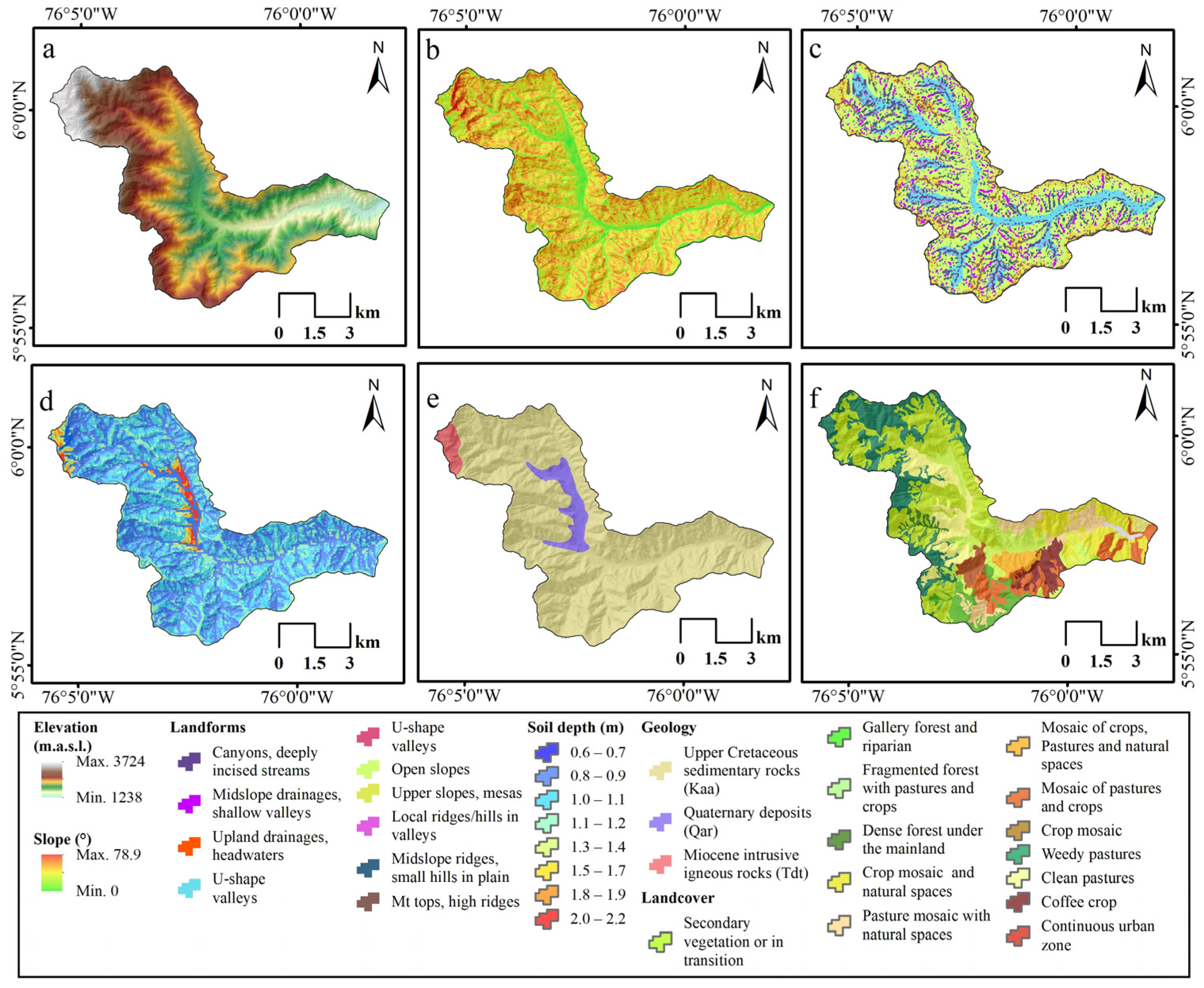
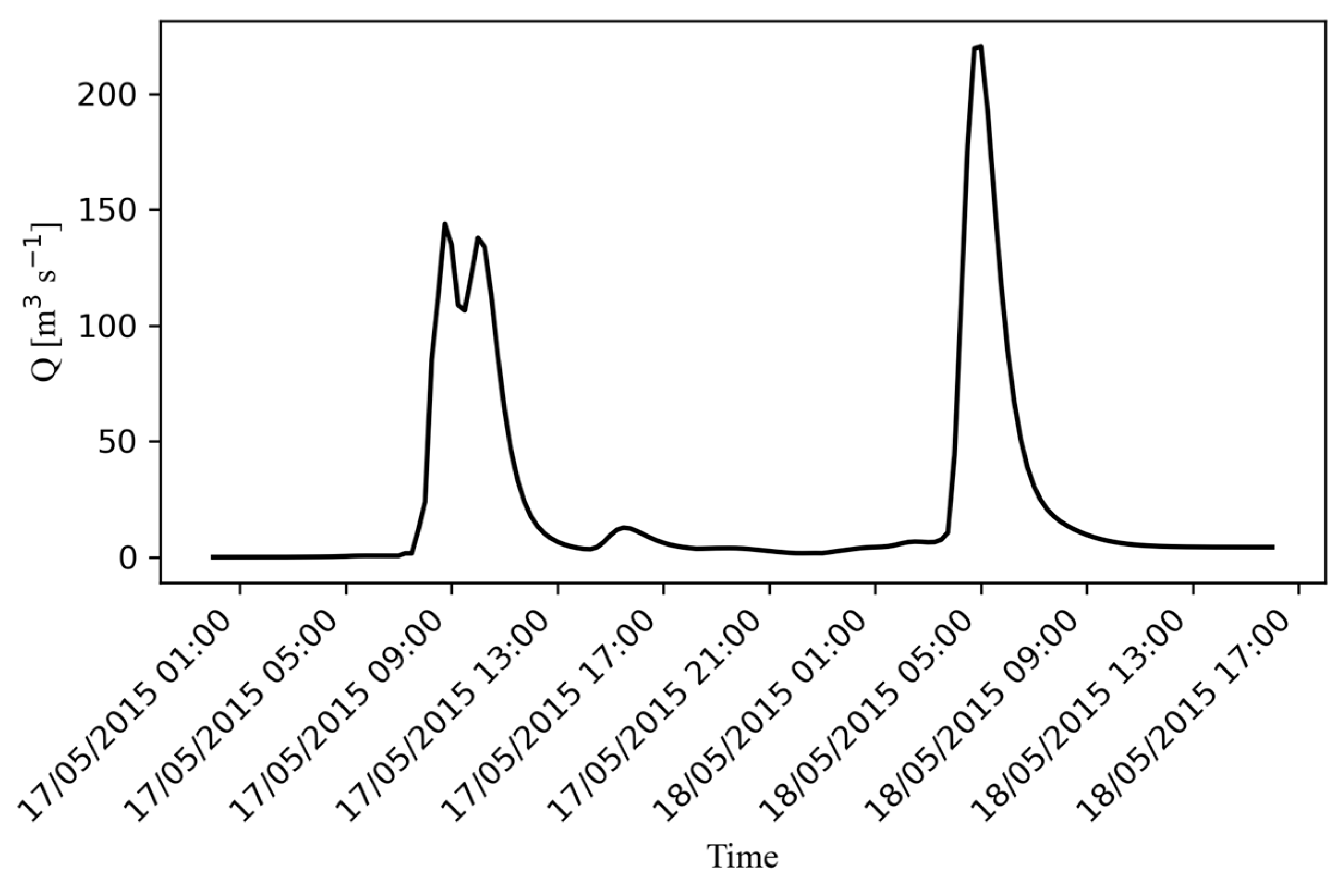
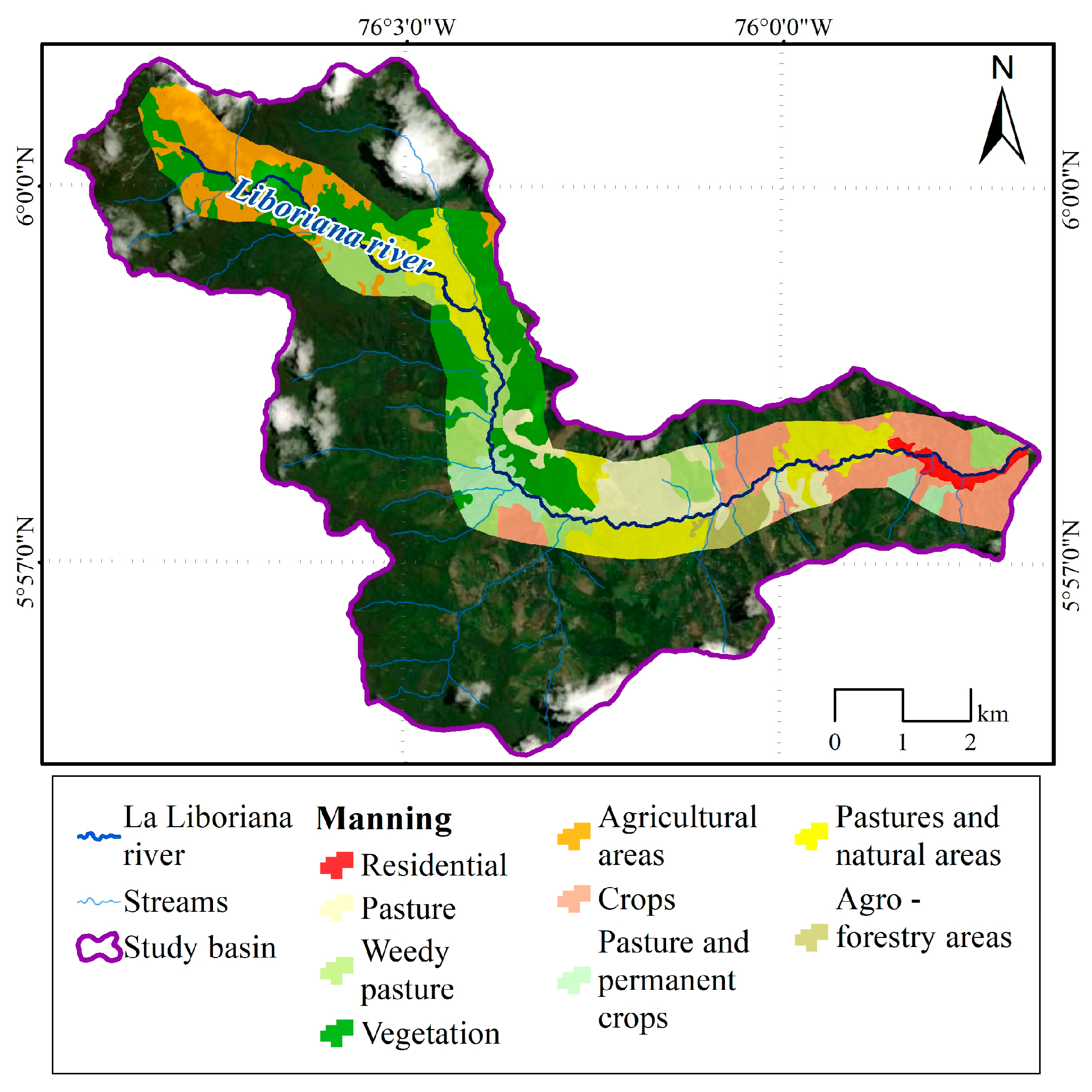
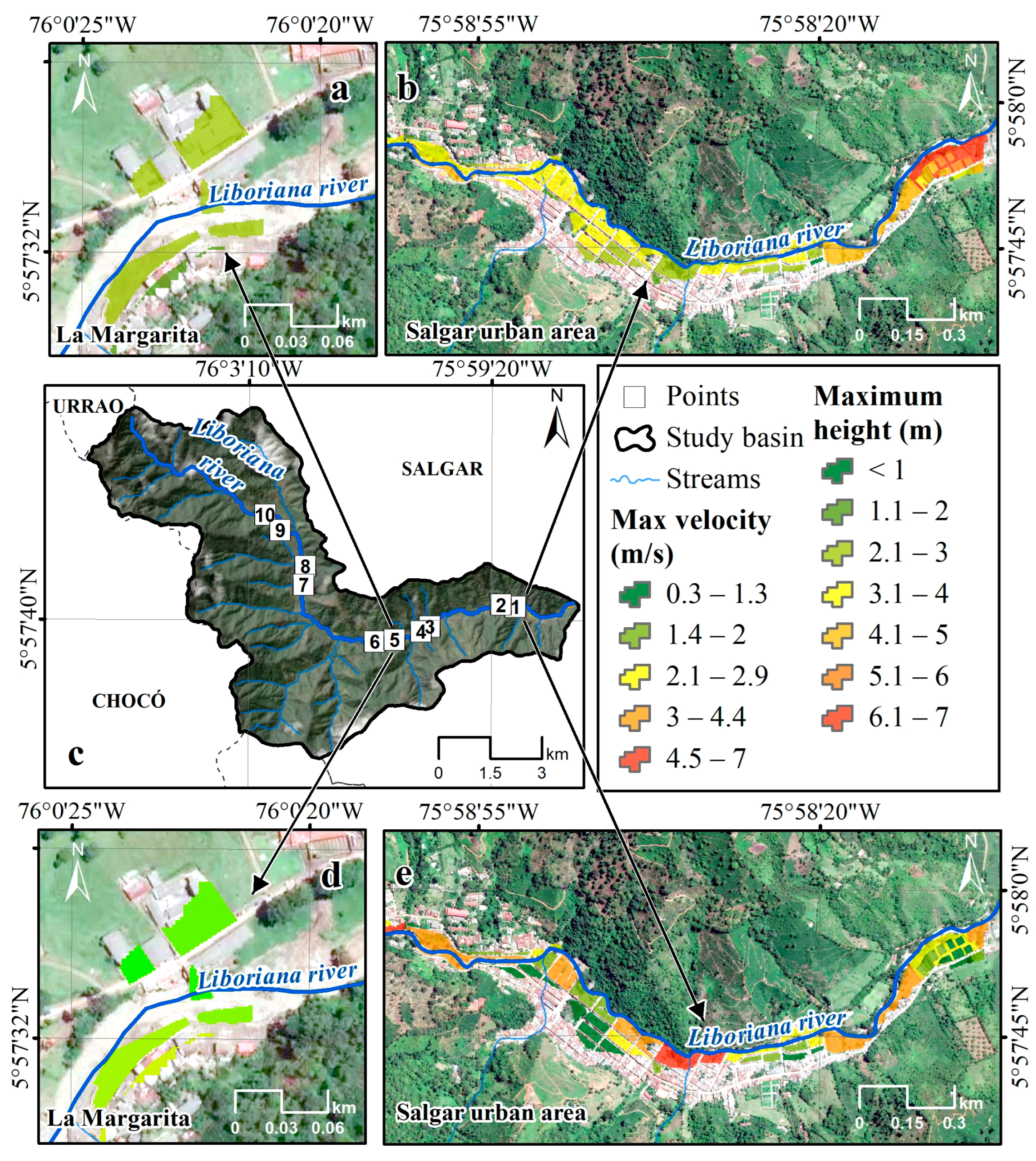
2. Study Area and Flash-Flooding Historical Event

The “La Liboriana” river basin was selected as a study area to explain and develop the proposed methodology. Located over the western branch of the Colombian Andes in the municipality of Salgar (southwest zone of the Department of Antioquia), as shown in Figure 1, the basin has an average elevation of 2487 m above sea level and 58.8 km² of surface (Figure 2a). The basin’s outlet lies 1316 m above sea level. The mainstream’s Strahler–Horton order is 5, with a length close to 19 km and a slope of 8.1%. Notably, approximately half of the basin’s total area exhibits slope gradients exceeding 30 degrees (Figure 2b), making it highly susceptible to landslides and soil erosion. The steep slopes, combined with the high variability of rainfall patterns and the presence of human activities in the lower and middle zones, increase the landslide risk and soil erosion in the basin.

Significant variability exists in the rainfall pattern at the both inter-annual and inter-seasonal scales. The rainfall regime in the area is bimodal, with peak rainfall occurring in May and October [30]. The average annual rainfall stands at 3073 mm, with rainfall data obtained from the Institute of Hydrology, Meteorology, and Environmental Studies (IDEAM) data portal.

The basin exhibits a mountainous landscape with a rugged topography, featuring narrow valleys and very steep forested slopes, particularly in the upper region (Figure 2c). From a geological perspective, the basin is mainly composed of a Cretaceous sedimentary rock formation, an intrusive body, and Quaternary deposits (refer to Figure 2e). The sedimentary rocks are part of the Urrao member of the Penderisco formation, which is the primary constituent of a roughly 5 km thick sequence of turbiditic arenites and mudstones [30]. These rocks have undergone extensive in situ weathering due to the humid tropical climate, resulting in the formation of well-developed saprolite and residual soils of several textures, with a predominance of limes and clays [31]. These soils are well drained, with poor retention capacity. In the first layer, organic material is predominant, and clay loam soil is present within the second one. The basin’s upper zone is dominated by dense tropical forests and agricultural crop fields, while the lower and middle zones have been transformed by human activities, with grasslands, coffee, and banana plantations replacing the original forests (Figure 2f). Moreover, grazing areas and urban development are located adjacent to the riverbanks, increasing the risk of soil erosion and landslides.

The geological data for this study area were obtained and digitized from 1:100,000 scale geological maps provided by the Colombian Institute of Geology and Mining (Colombian Geological Service). The land cover classes were extracted from a 1:100,000 scale land cover map produced by the IDEAM for the years 2005–2009, following the CORINE Land Cover Colombia (CLC) methodology (see Figure 2f). The digital elevation model (DEM) was generated using cartographic data from the Colombian Geographic Institute Agustín Codazzi (IGAC), with a spatial resolution of 10 m.

On 18 May 2015, the La Liboriana basin and the municipality of Salgar in Colombia experienced a devastating natural disaster due to heavy rainfall. The rainfall’s intensity caused many landslides in the area, displacing regolith soil and exposing the underlying rock formation. The SIATA weather radar (Early Warning System for Medellín and the Aburrá Valley) recorded a significant rainfall event between 10:00 p.m. on 17 May and 2:00 a.m. on 18 May. The western zone of the basin was especially impacted, with heavy rainfall affecting around 30% of the basin’s total area. During this four-hour period, the rainfall accumulation reached 100 mm, with minor rainfalls continuing until 7:00 p.m. on 18 May. In total, the upper part of the basin received 160 mm of rainfall within 24 h. This continuous rainfall triggered around 160 shallow landslides in the area, with 50 specifically identified and recorded in the basin. The combination of heavy rainfall and the basin’s vulnerable geological conditions contributed to the occurrence of these landslides [32]. In the early morning hours, the intense rainfall also triggered landslides in the basin and caused the river to overflow, leading to a blockage of the stream [33]. When the natural dam broke, more than 100 people lost their lives, and many others were reported missing. Houses, bridges, and roads were destroyed, leaving hundreds of people homeless and severely impacting the local infrastructure.

3. Materials and Methods

This study analyzes two types of mass movements, shallow slides (movement of cohesive soil masses along a defined sliding surface) and their associated debris flows (fluid-like movement of coarse earth material), in accordance with the Varnes landslide classification detailed by Hungr et al. [20]. The proposed methodology for assessing landslide hazards in the La Liboriana basin follows a multi-model approach, as outlined in Figure 3. The first step involves using the SLIDE model [34], a physically based landslides prediction model, to evaluate the spatial distribution of rainfall-induced shallow landslide hazards, as expressed as the Factor of Safety (FoS). This model requires input data such as the intensity–duration–frequency (IDF) curves, soil depth, and soil hydro-geomechanical parameters. The second step is to simulate debris flow propagation using the RAMMS model [35]. This model takes the release areas identified through the SLIDE hazard zoning as inputs, along with a digital elevation model (DEM) of the basin. The final step integrates the results of the previous models to assess the impact of river obstruction within the basin. This is performed using the IBER model [36], which requires flow hydrographs obtained from the TETIS model [37] for various return periods, as well as the sliding material (deposition heights) in the form of modified DEMs derived from the RAMMS simulations. The overall methodology is based on automating spatial analysis and modeling processes in GIS software (ArcGIS Desktop 10.8), allowing for the integration of the various input parameters and the spatialization of the soil depth susceptible to landslides. Detailed descriptions of each methodological step are provided in the sections that follow.

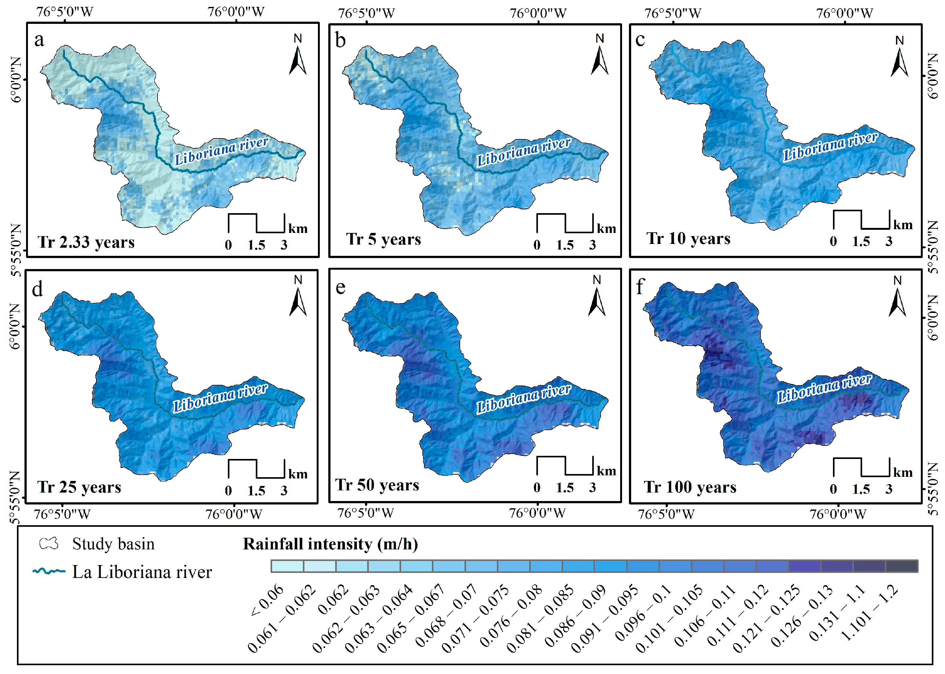
3.1. Spatial Rainfall Intensities

The study area is located within the coverage of the C-band polarimetric Doppler weather radar operated by the Early Warning System for Medellín and the Aburrá Valley (SIATA). For rainfall estimation, the radar has a radial optimal range of 120 km, and it has a maximum operational range of 240 km for weather detection. Located 65 km away from the basin, there are no blind spots for the radar [38]. Radar-based Quantitative Precipitation Estimation (QPE) is estimated from reflectivity (dBZ) through a relationship calibrated by SIATA using disdrometers and finding parameters according to orography. The radar QPE technique is described in Sepulveda [39] and, Sepúlveda and Hoyos [40]. We used intensity maps estimated from reflectivity retrieved from SIATA records, approximately every five minutes, from 2013 to 2021, at a pixel spatial resolution of 166 m. From the 5 min intensity maps, the intensities were obtained for durations of 10, 15, 30, 45 and 60 min. Subsequently, an annual maximum intensity map was obtained for each duration. A spatial fitting of the Gumbel and Log normal probability distribution functions was performed for each of the series of maximum intensities in each pixel. The Kolmogorov–Smirnov goodness of fit test was applied. The hypothesis that the data on the basin are adjusted to the two distributions is accepted. The values of the D statistic for the Lognormal are in some cases closer to the limit statistic; therefore, it was decided for the purposes of this paper to show the analysis and the IDF curves from the results of the Gumbel distribution fit. The result is a map of the parameters α and µ of the Gumbel distribution function for each pixel. This allows the calculation of intensity maps for any duration and return period.

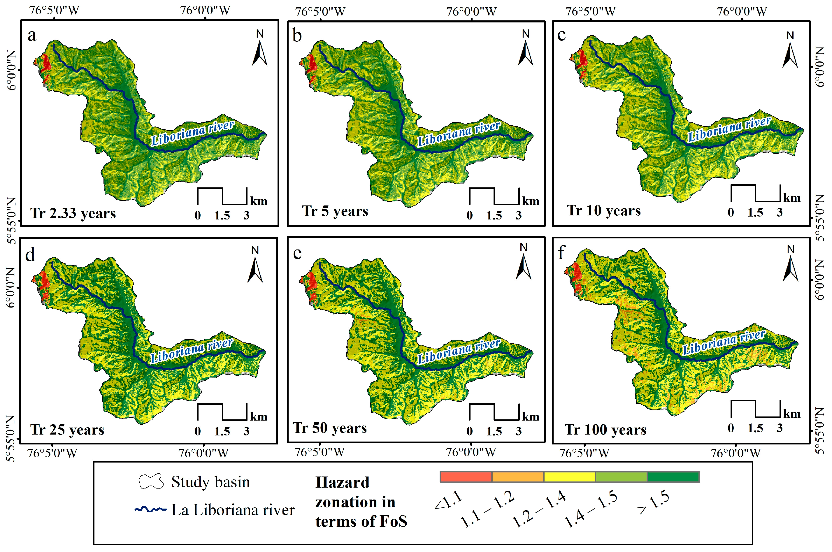
3.2. Landslide Hazard Assessment Using Slope–Infiltration–Distributed Equilibrium (SLIDE) Model

The spatial distribution of rainfall-induced landslide hazards, in terms of the Factor of Safety (FoS) values, was estimated using the SLIDE model, a deterministic model coupling the infinite slope model with an infiltration model. Developed based on the Transient Rainfall Infiltration and Grid-Based Regional Slope-Stability Analysis (TRIGRS) model from the Hydrometeorology and Remote Sensing Laboratory at the University of Oklahoma [41], the SLIDE model focuses on shallow landslides, identifying areas susceptible to failure based on the intrinsic soil parameters and the geomorphometric pattern of the terrain. The model simulates rainfall events as triggering factors and assesses the soil’s response to these events. The FoS is defined as the ratio of stabilizing forces to destabilizing forces, considering stable slopes when the FoS is ≥1 and instable slopes when the FoS < 1 [42]. In this study, high hazard zones were defined as those with an FoS < 1.1, presenting a conservative scenario [43].

Due to the complexity of shallow landslide studies, the SLIDE model incorporates the following simplifying assumptions: the slope is considered as infinite with minimal soil thickness, the failure plane is assumed to be flat, and the water flow occurs parallel to the slope. The model excludes evapotranspiration, underground seepage, and surface flow from the water balance. As a result, infiltration is approximately equal to the maximum saturated hydraulic conductivity [44]. The model adopts simplified assumptions regarding the water downflow and establishes a direct relationship between the FoS of slopes and rainfall intensity [45]. It underscores the destabilizing impact of the water downflow and highlights the role of partial saturation in enhancing the soil shear strength. The FoS is expressed through the following straightforward mathematical formulation:

$$\mathrm{F}\mathrm{o}\mathrm{S}={\displaystyle \frac{\mathrm{c}\mathrm{o}\mathrm{t} \mathrm{c}\mathrm{o}\mathrm{t}\mathsf{\beta } \mathrm{t}\mathrm{a}\mathrm{n} \mathrm{t}\mathrm{a}\mathrm{n}\mathsf{\varphi }\left[\mathrm{\Gamma }+{\mathrm{m}}_{\mathrm{t}}({\mathrm{n}}_{\mathrm{w}}-1)\right]+\mathrm{C}\mathsf{\Omega }}{\mathrm{\Gamma }+\mathrm{m}{\mathrm{n}}_{\mathrm{w}}}}$$

(1)

$$\mathrm{\Gamma }={\mathrm{G}}_{\mathrm{s}}\left(1-\mathrm{n}\right)+\mathrm{n}{\mathrm{S}}_{\mathrm{r}}$$

(2)

$${\mathrm{n}}_{\mathrm{w}}=\mathrm{n}(1-{\mathrm{S}}_{\mathrm{r}})$$

(3)

$$\mathsf{\Omega }={\displaystyle \frac{2}{\mathrm{s}\mathrm{i}\mathrm{n} \mathrm{s}\mathrm{i}\mathrm{n} 2\mathsf{\beta }\mathrm{Z}{\mathsf{\gamma }}_{\mathrm{w}}}}$$

(4)

where β is the slope angle [°], ϕ is the friction angle [°], C is the soil cohesion [kPa], and m_t is a dimensionless thickness of the saturated part of the soil layer. G_s is the specific gravity, n is the porosity, S_r is the degree of saturation [%], Z is the soil depth (thickness) [m] and γ_w is the unit weight of the water [kN/m³] [34,46]. Γ (Equation (2)) is a variable introducing consistently, the variables representing the soil properties, while Ω (Equation (4)) involves the geometric variables susceptible to sliding.

The parameter m_t is the link between the saturated part of the soil layer and rainfall with the FoS, which is a fractional parameter between 0 and 1, and during numerical simulation it could be derived by calculation of the water balance at each time step (Equations (6) and (7)) [30]. The initial value of m₁ could be determined by an in-situ test of the water table or from the assumption of this value according to the knowledge of the study area. O_t represents the water outlet of a finite portion of a slope of finite length calculated by Equation (5) [34]:

$${\mathrm{O}}_{\mathrm{t}}=\mathrm{K}\sin \mathsf{\beta }{\mathrm{m}}_{\mathrm{t}}\mathrm{Z}\cos \mathsf{\beta }∆\mathrm{t}$$

(5)

$$∆{\mathrm{m}}_{\mathrm{t}}={\displaystyle \frac{({\mathrm{I}}_{\mathrm{t}}-{\mathrm{O}}_{\mathrm{t}})}{\mathrm{n}\mathrm{Z}(1-{\mathrm{S}}_{\mathrm{r}})}}$$

(6)

$${\mathrm{m}}_{\mathrm{t}+1}={\mathrm{m}}_{\mathrm{t}}+∆{\mathrm{m}}_{\mathrm{t}}$$

(7)

where K is the hydraulic conductivity of saturated soil [m/h], t is the time [h], and Δt is the time step m. The initial values of m and m_t are calculated at each time step. I_t is the rainfall intensity [m/h] and m₁ is supposed to be 0.3 in the study basin.

Figure 2d illustrates the spatial distribution of geological units in the study basin and

Table 1. Soil hydro-mechanical properties used in the SLIDE model. Source: Marín et al. [30].

Lithology	Nomenclature	C	ϕ	Gs	n	Sr	K
Upper cretaceous sedimentary rocks	Kaa	10.5	24.0	2.68	0.40	65.0	3.98∙10−3
Quaternary deposits	Qar	18.0	30.0	2.65	0.39	70.0	1.80∙10−2
Miocene intrusive igneous rocks	Tdt	5.0	32.0	2.65	0.39	94.0	3.60∙10−2

provides a summary of the soil properties required for the SLIDE model and the estimated values for the soil depth. Relevant information on the geological formations in Table 1 is described in detail in Section 2.

The depth of the potentially unstable soil is a critical parameter that strongly influences the stability of slopes [47]. The evaluation of such soil thickness, susceptible to sliding or detachment, is essential before the analysis of problems involving hydrological processes developed on slopes, as well as slope stability [48]. The estimation of soil thickness is based on the soil’s behavior in relation to the terrain’s slope; high slopes imply less soil accumulation. The model of the soil susceptible to sliding is represented by the following equation [49]:

$$\mathrm{Z}=\left({\mathrm{z}}_{\mathrm{m}\mathrm{a}\mathrm{x}}-{\mathrm{z}}_{\mathrm{m}\mathrm{i}\mathrm{n}}\right)\times \left\{\left[1-{\displaystyle \frac{1}{\mathrm{t}\mathrm{a}\mathrm{n}\left({\mathsf{\beta }}_{\mathrm{l}\mathrm{i}\mathrm{m}}\right)}}\mathrm{t}\mathrm{a}\mathrm{n}\mathsf{\beta }\right]\times \left[\mathrm{t}\mathrm{a}\mathrm{n}\mathrm{h}\left(\mathrm{a}\mathrm{x}\right)\right]\right\}+{\mathrm{z}}_{\mathrm{m}\mathrm{i}\mathrm{n}}$$

(8)

where Z is the soil depth (thickness) [m], z_max is the maximum soil thickness [m], z_min is the minimum soil thickness [m], β is the slope angle value [°], β_lim is the slope angle value threshold for which higher values imply that the thickness of soil susceptible to sliding is minimal/negligible or even null [°], and a is a dimensionless parameter that controls the estimation of the soil thickness depending on the curvature of the terrain. The values were chosen according to predominant soil types of the geological units in tropical zones. The curvature controls the zones of water accumulation or spreading, which directly influences the degree of soil moisture and/or saturation and, therefore, the generation of debris flows [50]. Finally, x is the horizontal distance from a reference cell to the nearest drainage. The hyperbolic tangent function (tanh) is utilized to compute the product ax, thereby inducing an interaction that governs the soil layer’s growth as a function of its horizontal distance from the nearest drainage point. As this distance increases, the propensity for soil layer thickening also increases. The integration of these two factors constitutes the proposed model for predicting the final soil layer thickness [49]. The minimum (z_min) and maximum (z_max) soil thickness for the geological units of Quaternary deposits and Miocene intrusive igneous rocks are 0.6 and 2.2 m, respectively. For upper Cretaceous sedimentary rocks, the assigned values are z_min = 0.8 m and z_max = 1.2 m.

The selection of the slope threshold in this research was performed after analyzing the statistics of the slope distribution within the study basin (Figure 2b). The mean slope angle is approximately 30°, with a standard deviation of around 11°. Therefore, it was decided to consider a critical value (β_lim) of 45°, slightly higher than the mean plus one standard deviation. The variable a was set to 0.04 [45]. Using map algebra through the ArcGIS platform, the relevant parameters were integrated to spatialize the model of soil depth (thickness) susceptible to landslides (Figure 2e).

3.3. Landslide Propagation and Deposition Height Modeling Using the Rapid Mass Movement Simulation (RAMMS) Software

The extent of the landslide footprint resulting from the sliding mass was evaluated using the RAMMS debris flow tool to obtain the landslide deposition heights and flow velocities. The release block methodology was employed based on the available data within the study basin, using a polygon layer of critical areas to delineate trigger zones. These release zones were demarcated from the hazard assessment methodology, specifically focusing on high hazard zones (FoS < 1.1), identified as described in Section 3.2.

The RAMMS model is governed by several equations, each of which depends on specific input parameters. These parameters include the flow height (H), gravity (g), slope angle (β) and Voellmy friction coefficients: dry Coulomb-type friction (μ) and turbulent viscous friction (ξ), among others [51]. These friction coefficients, μ and ξ, which remain constant and are user-defined, play a fundamental role in determining the debris flow characteristics within the RAMMS model [52]. The parameters required by the model are the density of the flow material and the Voellmy friction coefficients. Viscosity governs when the flow is about to stop or, in other words, when the kinetic energy of the flow is running out, while viscous–turbulent friction governs when the flow is moving fast [53]. Specifically, the parameter ξ dominates in fast debris flow scenarios, while μ dominates in near-static debris flow situations.

The RAMMS debris flow model considers the fluid flow as a single phase, uses a depth-averaged shallow water equation for granular flow modeling, and employs a Voellmy–fluid friction model as follows [54]:

$$\mathrm{S}=\mathsf{\mu }\mathsf{\rho }\mathrm{H}\mathrm{g}\mathrm{c}\mathrm{o}\mathrm{s}\mathsf{\beta }+\left({\displaystyle \frac{\mathsf{\rho }\mathrm{g}{\mathrm{u}}^2}{\mathsf{\xi }}}\right)$$

(9)

where S is the frictional resistance [Pa], $\rho$ is the density [kg/m³], g is the gravitational acceleration [kg/m²], β is the slope angle [°], H is the flow height [m] and u is the vector of the flow velocity in the x- and y-directions. The Voellmy model accounts for the resistance of the solid phase μ [Pa∙s], which is sometimes expressed as the tangent of the internal shear angle and a viscous or turbulent fluid phase ξ [m/s²].

During this stage, sensitivity analyses were conducted to calibrate the model, aiming for each parameter to reproduce the events that occurred on 18 May 2015. The sensitivity analysis involves adjusting the parameters of the model to find the optimal values that can accurately simulate real-world events. In the case of RAMMS, a total of 30 simulations were executed. As previously explained, according to the input parameters of the application, which include the DEM, the landslide initiation sources (release areas), the probable sliding soil depth, and the rheological parameters of the soil (viscosity and turbulent friction coefficient), the number of simulations to be performed was determined.

Since the parameters related to the terrain and the initiation of landslides were the same for all the simulations, the parameters that were varied included the viscosity, turbulent friction coefficient, and soil depth. The RAMMS user manual suggests that, for a debris flow case, the viscosity (μ) values should be between 0.05 and 0.4 Pa∙s, and the turbulent friction coefficient (ξ) should be between 200 and 1000 m/s². However, it was decided to adjust the soil viscosity values above the upper range, as the sensitivity and trial-and-error approach with the application indicated that values within this range did not adequately describe the soils present in the study area basin. Therefore, a range of viscosity values between 0.5 and 0.7 Pa∙s was used. Regarding density, a value of 2000 kg/m³ was adopted, according to the user manual recommendation, similar to the values reported in Vega and Hidalgo [32] for the soil density in the upper zone of the basin from secondaries sources.

With the deposition heights estimated with the RAMMS debris flow modeling, some of them in the river channel, the digital elevation model (DEM) is modified for each return period, allowing us to represent the partial or total obstruction of the channel. These modified DEMs are used in hydraulic modeling to show the change in the behavior of the flow and flooding for several return periods as follows.

3.4. Probabilistic Torrential Flood Hazard Zonation

As a crucial step in the methodology proposed in this paper, the torrential flood hazard is zoned based on the hydrographs associated with the same triggering intensities of the debris flow and its propagation. The different results of the propagation are transformed into different river channel obstructions associated with the same return periods. These results are finally used for hydraulic modeling to obtain the different probabilistic flood zones. The assumptions and models used in this final stage of the methodology are described below.

For hydrological modeling, the distributed TETIS model is calibrated using event-based temporal resolution. Subsequently, the resulting hydrograph for each spatially distributed intensity is simulated for the considered return periods. The TETIS model [37], a conceptual and distributed model, has been successfully employed in mountainous regions for simulating flood events [55]. Implementing the TETIS model requires data derived from the DEM, soil hydraulic parameters, and vegetation cover. As a distributed model, TETIS effectively captures the spatial distribution of rainfall, which is critical for the study area. This capability allows for the generation of flow hydrographs at various tributary entry points into the main channel, thereby enabling more accurate hydraulic modeling.

The hydraulic modeling is carried out using the numerical hydraulic model IBER [36,56]. The software follows a detailed and robust methodology for the hydraulic modeling of free sheet flow in rivers and estuaries. It uses an approach based on the Shallow Water Equations that integrates continuity and quantity of motion in two dimensions. IBER begins with the collection and input of topographic, bathymetric and land-use data, followed by the definition of the boundary conditions and hydraulic properties of the terrain, such as the roughness coefficients. The software then employs a finite volume numerical scheme to solve the flow equations, allowing us to simulate the propagation of the flood wave over time and space. During this process, calibrations and validations are performed by comparing simulated results with observed data, adjusting the model parameters to improve the model accuracy. The model output includes maps of the depth, water velocity and flood extent, which are essential for hydraulic risk planning and management.

IBER requires as the initial input a three-dimensional terrain model or mesh. This is derived from the modified and original DEMs. It also requires the incorporation of the boundary conditions, initial conditions, and the assignment of terrain roughness coefficients. The hydrographs obtained for each return period are incorporated into the hydraulic model at the locations where significant tributaries join the main channel. Model calibration is performed using the water levels reported during the historic torrential flood event of 18 May 2015.

In a hydraulic study of a flood, the relationship between the type of land cover and the roughness coefficient is critical in determining the accuracy of the flow models. Land covers, such as urban areas, forests, agricultural fields, and water bodies, significantly affect the resistance to water flow. Each type of cover has a specific roughness coefficient, known as Manning’s coefficient, which quantifies this resistance. For example, urban areas with paved surfaces have a low roughness coefficient, allowing water to flow faster, while dense forests have a higher coefficient, slowing the water flow. The correct assignment of these coefficients in the hydraulic model is crucial for accurately predicting flood zones and flow dynamics during flood events.

In the same type of study, the importance of having calibration points with known water height data is crucial to the accuracy of the hydraulic model. These calibration points allow the model to be adjusted and validated by comparing the simulated water heights with the observed water heights, ensuring that the model accurately reflects the reality of the terrain and flow behavior during flood events. Water height information helps identify and correct potential errors in the topography and model hydraulic parameters, such as the roughness coefficients. Without accurate water height data, the model may fail to adequately predict flooded areas, which can lead to ineffective flood risk management and implementation of inadequate mitigation measures. Therefore, known water height data are essential to ensure the reliability and usefulness of the hydraulic model in flood planning and response. For this work, we used 10 control points obtained from the study by Velásquez et al. [38] and whose information is shown in Section 4.4.

4. Results

To apply the described methodology, return periods of 2.33, 5, 10, 25, 50 and 100 years were defined. These return periods were maintained for each step of the methodology, as described above.

4.1. Spatial Rainfall Intensities for Each Return Period

Figure 4 presents maps showing the spatial distribution of the rainfall intensity across the basin for various return periods (Tr): 2.33, 5, 10, 25, 50, and 100 years. Each map illustrates the intensity of rainfall (in meters per hour) across the basin, with varying shades of blue representing different intensity ranges. These maps were obtained for a duration equal to the basin concentration time calculated in 96 min (Figure 4). The maximum intensities were highly concentrated in the northwestern upper basin and in the southeastern zone of the lower basin.

As the return period increases, the overall rainfall intensity across the basin also increases. Higher return periods (50 and 100 years) show more pronounced and widespread high-intensity rainfall areas, especially in the upper and lower parts of the basin. These maps provide a clear visualization of how the rainfall intensity varies spatially and increases with longer return periods, which is crucial for understanding flood and landslide risks in the region. Increasing rainfall intensities over time will impact landslides, as seen in the following section.

4.2. Landslide Hazard Assessment

To validate and calibrate the stability model described in Section 3.2, we performed a comparison with the inventory of failure zones generated by the 18 May 2015 event using the receiver operating characteristic (ROC) analysis technique. The prediction rate of the calibration model was just over the random prediction, with an area under the ROC curve (AUC) equal to 0.60. Subsequently, using the parameters adjusted in the calibration, we performed an analysis for different return periods. A total of six landslide hazard maps in terms of the FoS were obtained. Figure 5 shows hazard maps for the basin, illustrating areas of varying stability based on the Factor of Safety (FoS) for the same return periods as the rainfall intensities. The maps use color-coding to represent different FoS ranges, indicating levels of landslide hazard. As the return period increases, the extent of high-hazard zones (FoS < 1.1) also increases, indicating a higher risk of landslides. The northern part of the basin consistently shows higher hazard levels across all the return periods, with increasing instability as the return period lengthens.

Critical stability zones were identified as areas with Factor of Safety (FoS) values less than 1.1. These zones are primarily located in the upper regions of the basin, where the average FoS is approximately 0.81. They are typically found on steep slopes with inclinations greater than 35°, at elevations ranging from 3027 to 3703 m above sea level. The average soil thickness in these critical zones is about 1.0 m. Geomorphologically, these areas are characterized by upper and open slopes, mountain tops, and high ridges. To a lesser extent, they also occur in midslope drainages and shallow valleys. Regarding land cover, the critical stability zones are predominantly found in gallery forests and riparian areas, as well as in dense highland forests. Regarding lithological units, these zones are primarily associated with the Tdt formation (pyroxene dioritic stock) in escarpment regions. In contrast, they are less frequently found in the Kaa formation, which comprises interstratifications of shales, siltstones, mudstones, sandstones, cherts, and polymictic conglomerates, in body and landslide deposition zones.

4.3. Landslide Propagation and Probabilistic River Channel Obstructions

Figure 6 displays maps of the La Liboriana basin showing the maximum deposition heights for the considered return periods according to the propagation modeling using RAMMS. The deposition heights are color-coded, with varying shades representing different height ranges (in meters). The calibration process of the propagation modeling was conducted considering the landslide footprints of the 18 May 2015 event and the process followed in Hurtado [57]. As mentioned in the Materials and Methods section, the probability associated with each of these deposition height conditions is associated with the probability of the triggering rainfall intensity and the critical stability conditions (FoS < 1.1) identified using the SLIDE model.

The simulation that produced the best results considered a viscosity value of 0.7 Pa∙s and viscous–turbulent friction coefficient of 1000 m/s². These two parameters describe the behavior of the flow. The results obtained correspond to the maximum deposition height of the flow. Evidently, the lowest deposition thicknesses occur in the steepest areas in the upper part of the basin (Figure 2b), while the highest values occur at the confluence with the streams.

The deposition heights increase with longer return periods, indicating more significant material accumulation during extreme events. The river channel consistently shows high deposition heights across all the return periods, reflecting its role in transporting and depositing materials. The northern and northwestern parts of the basin are particularly prone to high deposition, especially for longer return periods. These maps are crucial for understanding the sediment dynamics and potential impacts on river morphology and infrastructure.

In river channel cells (pixels), these deposition heights create partial obstructions within the river. As illustrated in Figure 7, there is a specific zone along a river section where the maximum deposition occurs, located around 18 km upstream from the outlet. This results in a 3 m obstruction or elevation increase in the riverbed between the original DEM and the Tr 2.33 DEM. The difference in the bed elevation between the 100-year return period and the 2.33-year return period is approximately 80 cm.

4.4. Hydrologic and Hydraulic Modeling

The flood hydrographs associated with each return period were simulated using the TETIS model with a 5 min time step, and the calibration event was simulated with a time step of 15 min. The spatial resolution for the model was consistent with that of the DEM used.

First, the model was calibrated to reproduce the hydrograph of the event. At the time of the torrential flood, there were no records of the water levels or flows at the outlet of the study basin and nowhere along the river. However, based on photographs, surveys and in situ evidence of the levels reached by the river during the event, some reconstructions of the flow hydrograph have been estimated and published. The parameters of the TETIS model have been calibrated satisfactorily, based on the reconstruction performed by Velazquez et al. [38], which also agrees with what was reported by the affected people and by in situ observations days after the disaster.

For the rainfall during the event, we used the intensity maps estimated from the reflectivity, approximately every five minutes from 16 May at 22:00 to 20 May at 6:00. The rainfall event had a high concentration of precipitation in the upper watershed area to the northwest, with values of the accumulated rainfall depth of 150 mm that even exceeded the maximum values of rainfall accumulated for a 100-year return period (Figure 8). The spatial distribution of the calculated intensities has been adjusted by a weighting process, without affecting the magnitude, to match the spatial distribution pattern of the calibration event. From the intensity maps of each return period, an event hyetograph was obtained in each cell, using the 50% probability distribution pattern for the first quartile of Huff [58], resulting in an incremental rainfall map, in time intervals in which the event was discretized, with the total duration time as the time of concentration of the basin (Figure 8).

The cumulative rainfall for the basin-wide event exceeds the cumulative probabilistic events for the entire basin obtained using the common hydrologic design approach. Given this result, the rainfall event would be much larger than the 100-year return period event for the entire basin.

The hydrograph resulting from the calibration is shown in Figure 9. The basin responds with two hydrographs separated by an interval of 20 h, with the last hydrograph being the one with the largest magnitude. The maximum flow values obtained in the modeling of the present work are 140 m³/s and 220 m³/s, while in Velásquez et al. [38], maximum flow values of 160 m³/s and 220 m³/s were obtained.

The response of the basin to the probabilistic events was simulated with the calibrated model. The hydrographs were obtained at some extra points at the outlet to cover the basin’s upper and lower parts. To select the tributaries that could be representative, the Horton and Strahler order was used as a criterion, and the points were marked on the branches of a number immediately below that of the main channel (Figure 8).

When simulating the torrential flood event and the probabilistic events, it is evident that the event on 18 May resulted from rainfall exceeding the maximum levels of probabilistic events across the basin. This is confirmed by the maximum flows obtained at the simulation sites for both the probabilistic events and the torrential flood event (

Table 2. Simulated flows for the torrential flood event and probabilistic events.

Simulation Site	Q Tr 5 [m3 s−1]	Q Tr 10 [m3 s−1]	Q Tr 25 [m3 s−1]	Q Tr 50 [m3 s−1]	Q Tr 100 [m3 s−1]	Torrential Flood Event
1	1.9	2.6	3.2	3.7	4.1	12.05
2	1.1	1.9	3.3	4.3	5.3	22.6
4	0.03	0.03	0.072	0.3	0.7	20.4
5	0.03	0.03	0.03	0.3	1.8	36.6
8	0.04	0.2	1.7	3.01	5.1	26.9
Outlet	6.3	8.6	12.4	16.3	22.5	220.4

). Only the magnitude of point 1 could be compared with the 100-year return period flow for this part of the basin. For the other sites, the flows are not comparable in magnitude. Some flows in Table 2 appear identical for different return periods because the variation in magnitude is not discernible with the decimal precision used in the table.

Hydraulic modeling was performed using the IBER model, as detailed in the Materials and Methods section. The roughness of the flood zone (see Figure 10) was determined based on the land cover. A mesh derived from the modified DEMs for each return period was utilized, and a time step of 1 s was applied. The modeled reach extends 19 km upstream from the basin outlet. The flood event was used to calibrate the model using the flow elevations reported by Velazquez et al. [38] for various locations along the study reach (Figure 8). The flow hydrograph at the reach outlet, obtained through hydraulic routing from the beginning of the reach and considering contributions from various tributaries along the river, aligns with the hydrologic model hydrograph at the outlet, indicating satisfactory performance of the hydraulic model (see Figure 11). Furthermore, as shown in

Table 3. Comparison of the water heights reported by Velasquez et al. [38] and simulated using the IBER model.

Site	Water Height from Velasquez et al. [38] [m]	Water Height from IBER Model [m]
1	4.00	4.05
2	4.00	4.02
3	2.60	2.50
4	4.00	3.42
5	4.00	4.05
6	1.04	1.06
7	0.52	0.53
8	4.00	2.42
9	0.52	0.60
10	2.08	2.03

, the hydraulic model for the event accurately reproduces the water levels reported by Velazquez et al. [38], which were verified in situ by post-event surveys and field evidence.

Figure 10 shows the different cover types along the lateral planes of the La Liboriana river and their association with various Manning’s ratios. A variety of coverages are observed, including residential areas, pastures, vegetation, agricultural crops and agroforestry zones. Residential areas, marked in red, typically have a low Manning’s coefficient due to the paved surfaces and structures that facilitate water flow. In contrast, areas of dense vegetation and agroforestry, represented in shades of green, typically have a higher Manning’s coefficient, reflecting the greater resistance to flow due to the presence of trees, shrubs, and uncompacted soil. Grassland and cropland areas, shown in yellow and orange, respectively, have intermediate Manning’s coefficients, as these terrains offer moderate resistance to water flow. This variability in the cover types and their respective Manning’s coefficients is crucial for the accurate modeling of water flows and the prediction of flood zones in the study area of the La Liboriana river.

The spatial distribution of the water level calibration points in the study, along the main channel of the La Liboriana river, extends uniformly from the upper to the lower reaches of the river (see Figure 12). In total, ten calibration points are identified, marked with numbers on the map (Figure 12c). The points are strategically located to capture a variety of hydraulic and topographic conditions. In the river’s upper reach, calibration points 9 and 10 are near the headwaters, ensuring calibration in the flow initiation areas. As the river advances toward the middle reach, points 6, 7 and 8 provide crucial data for this intermediate section. Finally, in the lower reach, points 1 to 5 are distributed along the channel, covering both areas near the mouth and more inland sections. This distribution allows accurate monitoring and calibration of the hydraulic behavior of the river in different segments, ensuring that the model adequately represents variations in the flow and height along the entire main channel.

In the comparative Figure 11, between the IBER and TETIS models, it is observed that both models show similar behavior in terms of the flow evolution over time. However, there are notable differences in the magnitude and shape of the flow peaks. During the first 60,000 s, the TETIS model presents more pronounced flow peaks compared to the IBER model, indicating a faster response and possibly more sensitivity to the initial rainfall events. On the other hand, in the interval near 100,000 s, both models converge and show an almost identical peak flow in terms of the height and duration, suggesting an alignment in the prediction of peak flow during the main flood event. In general, the TETIS model tends to show sharper fluctuations and slightly higher peak flows in the initial phases of the hydrograph, while the IBER model shows a more smooth and moderate response in these same periods.

Table 3 shows a comparison of the water levels at various sites along the La Liboriana river according to two sources: Velasquez et al. [38] and the IBER model. The results indicate that, in general, the water levels estimated by the IBER model are similar to those reported by Velasquez et al. [38], with some differences at certain points. For example, at site 1, both studies show remarkably close levels (4.00 m vs. 4.05 m), suggesting good agreement. However, at site 4, there is a more significant difference, with Velasquez et al. reporting 4.00 m and the IBER model estimating 3.42 m, which may indicate variations in the input data or in the methodology used. Sites such as site 8 also have significant discrepancies (4.00 m vs. 2.42 m), highlighting the need for a detailed review to understand the causes of these differences. The points 6–10 are specific sites in areas where the geologic and topographic information was less detailed. Overall, the table suggests that, although the IBER model is consistent with the results of Velasquez et al., there are specific areas that require further investigation to ensure accuracy in modeling water levels.

During the torrential flood event on 18 May, the greatest damage was reported in two areas, as shown in Figure 12. The first area, located upstream and known as La Margarita, experienced water heights ranging from 3 m to 4 m and velocities between 4 m/s and 5 m/s. The downstream area, in the urban region of Salgar, recorded water levels up to 6 m and velocities of 6.9 m/s during the event.

The spatial variation of the water height along the main channel of the La Liboriana river (see Figure 12 (top)) in the modeled event shows significant differences, especially when analyzing the urban sections. In general, the water height level varies between 0.23 and 7.00 m. In the urban sections, as observed in the sectors near the city of Salgar, the water height level reaches higher values, in the range of 4.01 to 7.00 m, indicated in yellow and red tones on the map. This indicates a considerable risk of flooding in these densely populated areas, where the urban infrastructure can influence the behavior of the flow, causing deeper water accumulations. On the other hand, in rural and less developed reaches, the water heights levels are generally lower, ranging from 0.23 to 4.00 m, represented in green and light-yellow colors.

For the same modeled event, the spatial variation of the maximum water velocities along the main channel of the La Liboriana river, according to the Figure 12 (bottom), shows a significant range of velocities ranging from 0.34 m/s to 6.98 m/s. In the urban sections, especially in the vicinity of the city of Salgar, areas with higher maximum velocities are observed, represented in red and yellow colors on the map, indicating values higher than 5.00 m/s. These high velocities in urban areas are of concern, as they can increase the potential for erosion and damage to infrastructure. In contrast, rural and less developed reaches along the river channel have lower velocities, generally in the range of 0.34 m/s to 3.00 m/s, indicated in light green.

4.5. Probabilistic Torrential Flood Hazard Zonation Results

Using the DEMs that were modified according to the deposition heights for each return period, we obtained the probabilistic flood zoning. This zoning specifies the maximum water levels and velocities reached for each return period.

The spatial variation of the water heights along the main channel of the La Liboriana river, for a simulation with a return period of 100 years, shows significant differences, especially in the urban sections. In Figure 13 (top), the water heights are represented by various color ranges. In the urban areas, specifically near Salgar, the water heights reach high values, between 3.01 and 6.00 m, indicated in orange and yellow tones. These urban areas are particularly vulnerable to severe flooding due to the concentration of infrastructure and buildings that can obstruct the natural flow of water, thus increasing the depth of the water table. In contrast, in the rural and less developed stretches, the water heights are lower, varying between 0.23 and 3.00 m, represented in shades of green and light green. In Figure 13 (bottom), the water velocities are represented in assorted color ranges. In the urban reaches, especially near Salgar, higher maximum velocities are observed, between 2.79 and 3.57 m/s, indicated in shades of red and orange. These high velocities in urban areas are of concern, as they can increase the potential for erosion and damage to infrastructure. In addition, these high velocities reflect how urbanization can accelerate the water flow due to lower soil permeability and the presence of structures that channel water quickly. In contrast, in rural and less developed reaches, the water velocities are lower, generally in the range of 0.16 to 1.75 m/s, represented in green and yellow.

5. Discussion

Figure 4 presents maps of the rainfall intensities for different return periods: 2.33 years, 5 years, 10 years, 25 years, 50 years and 100 years. Analyzing the spatial distribution of the intensities in the La Liboriana river basin, we observed significant patterns of variation as the return period increases, clearly differentiating the high, intermediate and low zones of the basin. For the return period of 2.33 years (Tr 2.33), the rainfall intensity is relatively low and uniform, with values between 0.69 and 0.81 m/h in most of the basin. The high (top left), intermediate (bottom center) and low (right) areas show a homogeneous distribution of rainfall intensities. With a return period of 5 years (Tr 5), the rainfall intensities increase slightly, standing between 0.81 and 0.93 m/h. Although the distribution remains quite uniform, a slight increase in the intensities is beginning to be noticed in the lower areas of the basin.

For the 10-year return period (Tr 10), the rainfall intensities increase even further, reaching values between 0.93 and 1.05 m/h. In this scenario, the low areas begin to show greater intensities of rainfall, while the high and intermediate areas maintain more moderate intensities. As the return period increases to 25 years (Tr 25) and 50 years (Tr 50), the rainfall intensities increase significantly, reaching between 1.05 and 1.17 m/h and 1.17 and 1.29 m/h, respectively. The low areas of the basin are the most affected, presenting the highest intensities, while the intermediate areas also show a notable increase. The high areas continue with more moderate but significant increases. Finally, for the 100-year return period (Tr 100), the rainfall intensities reach their maximum values, exceeding 1.29 m/h in several areas, especially in low areas. Thus, the low areas of the basin are the most affected by the highest rainfall intensities, followed by the intermediate areas, while the high areas present more moderate increases. This analysis highlights the importance of focusing flood risk mitigation and management strategies on the basin’s most vulnerable areas.

To validate the results of this study, we utilized data from the 18 May 2015 event, including information on the antecedent rainfall, scarp formations, flow paths, and flood-affected areas. This allowed us to compare our modeling outputs against real-world observations from this significant landslide and debris flow incident. This comparison showed that our integrated modeling approach produced results that align with the conclusions of previous investigations under certain scenarios and methodological approaches. Regarding the rainfall–landslides relationship, data from the “Sistema de Información de Movimientos en Masa” (SIMMA) landslide database of the Colombian Geological Service indicated that prior to the 2015 event, antecedent rainfall in the basin averaged around 40 mm, 130 mm, and 220 mm over 3, 15, and 30 days, respectively. During the first 4 h of the extreme downpour between 10:00 p.m. on 17 May and 2:00 a.m. on 18 May, the upper part of the basin experienced nearly the same amount of rainfall as the 15-day antecedent total, which undoubtedly had a significant impact on the slope stability.

The critical soil moisture saturation level for landslide initiation is closely related to both the antecedent rainfall and the physical characteristics of the soil in the basin. Based on previous events recorded in the SIMMA database and the significant impact observed during the 2015 extreme downpour, it is inferred that when the soil moisture reaches near saturation, likely approaching or exceeding 80–90% saturation, there is a heightened risk of slope failure in the basin. This saturation level is mainly reached after prolonged rainfall or intense short-duration storms, which reduce the shear strength of the soil, making it more susceptible to landslides. The observed data from the 2015 event suggest that the combination of high antecedent moisture levels and the intense rainfall was sufficient to push the soil moisture to this critical threshold, leading to slope instability in the upper part of the basin. Further detailed studies, including field measurements and/or simulations, would be necessary to establish a precise saturation threshold, but the evidence points to this range as a critical level for landslide formation in this specific area.

With respect to the landslide hazard assessment, some studies using physically based models have been carried out in the same area. Marin et al. [30] reported a model performance with an ROC (AUC) of approximately 0.80 for the entire basin and 0.56 for the upper basin using deterministic models (TRIGRS model). Similarly, Hidalgo and Vega [8] achieved an ROC (AUC) of 0.56 using the EPADYM (Evaluación Probabilística de la Amenaza por Deslizamientos y Movimientos en Masa, in Spanish)) model to estimate the failure probability and the factor of safety under both seismic and static conditions. Vega and Hidalgo [32] obtained an ROC (AUC) value of 0.60 with the TRIGRS model for landslide hazard mapping based on the same historical event in relation with the historical extreme rainfall event. It is important to note that the uncertainty of several parameters involved in the FoS calculation significantly impacts the predictive accuracy of the physically based model used. This becomes even more critical when many of these parameters are derived from secondary sources.

Considering others’ approaches, Aristizábal-Giraldo and Ruiz [31] achieved an ROC (AUC) of 0.69 using a multivariate statistical (logistic regression) analysis. In the same line, Vega and Hidalgo [32] reported ROC (AUC) values of 0.95 and 0.86 using the Support Vector Machine (SVM) and fuzzy gamma models, respectively, for landslide hazard mapping based on the same 2015 event. Moreover, Vega et al. [59] obtained ROC (AUC) values around 0.95 using ensembles of decision trees, such as Random Forest and Ranger, to handle high-dimensional data with the historical landslide inventory in this tropical mountain basin.

Regarding propagation modeling, according to the RAMMS user manual, viscosities greater than 0.4 typically do not yield effective simulation results, while small values of ξ are typically associated with granular flows and larger ξ values are sometimes linked to sludgy flows, requiring delicate calibration with suggested values ranging between 100 and 200 m/s² [35]. Nevertheless, the viscosity and coefficient of viscous–turbulent friction values used deviate from those recommended in the RAMMS user manual. This choice reflects the rheological characteristics and geomorphological conditions specific to the study area, and the RAMMS simulation effectively identified landslide propagation areas that closely aligned with the footprints of actual landslides, particularly in the upper zones or where the movement initiated. However, the model’s performance was notably poorer in areas where movement ceased or deposition occurred, showing limited correlation. Despite RAMMS allows different values of viscosity and viscous–turbulent friction to be considered within the same simulation, for this research, these variables were considered constant over time given the limitation of not having primary data and the spatial variability of the parameters.

To analyze the results of the simulations mentioned above, it was decided to start by analyzing the graphical matches between what happened and what was obtained with the simulations. Numerically, real landslides covered an area of 0.37 km², whereas those simulated by RAMMS spanned approximately twice that area. RAMMS demonstrated an overlap accuracy of around 40% with the evaluated areas, considering the calibration scenario using the historical event of 18 May [57].

The propagation modeling approach utilized in this study is subject to limitations. The viscosity values used in the debris flow simulations may not have been optimally adjusted from secondary sources, potentially leading to inaccurate trajectory predictions. Additionally, the assumption of a maximum 2.2 m soil depth without verified stratigraphic profiles introduces uncertainty and could underestimate the mobilized soil volume in some areas. The reliance on a geomorphology-based model, due to the lack of detailed stratigraphic data, also carries inherent uncertainties in the estimated debris volume. While two modeling approaches were tested, the best results were obtained using the methodology outlined previously [49]. Addressing these limitations using more refined viscosity parameters and the collection of detailed stratigraphic data would help improve the reliability of the modeling results.

The analyses reveal a clear relationship between the return periods of extreme precipitation events and the geomorphological response of the La Liboriana basin. The rainfall intensity maps indicate that the maximum intensities are concentrated in the northwestern and southeastern parts of the basin, significantly increasing with longer return periods. This intensification pattern suggests the heightened vulnerability of these areas to extreme rainfall events. A hazard zonation based on the Factor of Safety (FoS) shows that as the return period increases, the high-risk areas (FoS < 1.1) expand, particularly in the northern part of the basin. This highlights the growing instability of slopes with increasing rainfall, emphasizing the need for preventive approaches in landslide risk management.

Furthermore, the maximum deposition height maps indicate a significant increase in sediment accumulation along the river channel and adjacent areas as the return periods lengthen. This pattern implies a substantial alteration of the river channel morphology and potential flow obstructions, exacerbating the risks of flooding and secondary landslides. Together, these findings underscore the importance of integrating hydrological, geomorphological, and deposition models in risk assessment for tropical mountainous basins. A detailed understanding of how the rainfall intensity and topography influence the slope stability and sediment dynamics is crucial for developing effective mitigation strategies and sustainable land-use planning in regions prone to extreme hydrometeorological events. Moreover, the importance of having flood models fed by detailed digital elevation models cannot be underestimated. Realistic digital elevation models (DEMs) provide an accurate and detailed representation of the terrain’s topography, essential for accurately predicting the areas affected by a flood. These models allow for a more adjusted simulation of the water flow, more accurately identifying accumulation zones and preferential flow paths. In addition, the high resolution of DEMs helps capture minor topographic features that can significantly influence flood dynamics.

A significant disadvantage in attempting to model landslide dams derived from debris flow obstructions is the uncertainty surrounding their locations, volumes, and shapes. These parameters are typically unknown or assumed a priori, which can lead to inaccuracies in predictive models. The proposed methodology addresses this issue by generating landslide dams in a probabilistic manner, allowing for the estimation of their location, height, and shape. This approach enhances the accuracy and reliability of the models, providing a more robust framework for understanding and predicting the impact of river obstructions.

The probabilistic scenarios for rainfall triggering landslides indicate that the event on 18 May exceeded the 100-year rainfall values across the entire basin. These probabilistic rainfall estimates are based on traditional design methods, which assume an event duration equal to the concentration time of 96 min, whereas the actual event lasted for four hours. However, the maximum intensities for shorter durations are higher for the same return periods. From this perspective, the reference event, in terms of the rainfall intensities and precipitation, may have surpassed even the 100-year probabilistic design event.

On the other hand, regarding the water heights, a comparison of the results of the maximum values in the La Liboriana river for the modeled event and for a return period of 100 years reveals significant differences in the magnitude and spatial distribution of the flood heights. In Figure 12, corresponding to the event, the maximum water heights vary between 0.23 and 7 m. The most affected areas, with heights of 5.01 to 7.00 m, are represented in orange and red tones, and they are predominantly located in the urban stretches near Salgar, where infrastructure and urbanization increase the accumulation and flow of water. In contrast, the simulation for a 100-year return period shows maximum water heights varying between 0.23 and 6.00 m, with the highest heights (5.01 to 6.00 m) also concentrated in the urban reaches, although the extent of these areas is smaller compared to the general event image. Areas with heights between 3.01 and 4.00 m, represented in yellow tones, extend along the main channel, indicating significant but less severe flooding than in the event simulation.

Both simulations highlight the vulnerability of urban areas to flooding, although the magnitude of the maximum heights varies slightly. The 100-year simulation presents a more conservative scenario with lower maximum heights compared to the event simulation, which may be due to the different assumptions or initial conditions in the models. In any case, the need for robust mitigation measures in urban areas is evident for both scenarios to protect the population and infrastructure from flood impacts.

Summarizing the findings regarding the water levels, the comparison between the study conducted by Velasquez et al. [38] and the IBER model results shows a high consistency in most of the sites evaluated, which validates the effectiveness of the IBER model for estimating the water levels in the La Liboriana river. However, the significant discrepancies observed at some specific points, such as sites 4 and 8, highlight the need for a detailed review and adjustment of the input data and model methodology. These differences underscore the importance of ongoing calibration and validation of hydraulic models to improve their accuracy and reliability. Ultimately, these adjustments will allow for better flood risk management and more effective planning in the region.

The comparison of the maximum water velocities reveals notable differences in the flow dynamics of the La Liboriana river during general events and for a 100-year return period that are crucial for flood risk management. In the event analyzed, the maximum water velocities vary significantly along the channel, with some areas reaching high velocities that could be indicative of a more turbulent flow with greater erosion potential. In this scenario, higher maximum velocities are observed, especially in urban areas and near infrastructure, reflecting the influence of structures and less space for water expansion, which increases the risk of erosion and damage to infrastructure.

On the other hand, the simulation for a 100-year return period shows a pattern of maximum velocities that, although still indicating high velocities in certain urban sections, generally presents lower values compared to the those of the event simulation. The areas with higher velocities are mainly located in the river’s narrower, urbanized sections, where human structures can cause flow acceleration. However, the range of velocities is more uniform and slightly lower, which could suggest a more managed distribution of the water flow due to the specific conditions. These differences underscore the need to implement robust mitigation measures in urban areas for both scenarios, focusing on improving the drainage infrastructure and urban planning to manage high flow velocities and protect the population and their property from the destructive effects of flooding.

Considering the morphology and morphometry considerations, we used RAMMS to simulate the propagation of debris flows and deposition of material in the river channel, which modifies the topography and thus the channel capacity. The results of these simulations are integrated into the IBER hydraulic model to reflect the new channel and floodplain conditions. This allows the model to capture variations in the channel capacity due to material deposition, a crucial factor in flood flow depth and velocity.

Regarding to the impact of urbanization and micro-relief, it is pertinent to recognize that the urbanization and micro-relief of the floodplain landscape can complicate the overall picture. In the IBER model, different roughness coefficients were incorporated to reflect the diversity in landcover types, including urbanized and agricultural areas. These coefficients were calibrated using historical water level data for an extreme and exceptional event to improve the accuracy in the representation of the water flow and its interactions with infrastructure.

Finally, in terms of the flood flow velocity and destruction, in areas where the flow capacity is reduced due to obstructions, our results show an increase in the flood flow depth and velocity. Simulations have shown that in some areas, the flow velocities also increase significantly, contributing to an increased risk of erosion and damage to infrastructure.

6. Conclusions

This study emphasizes the significance of cascade modeling for understanding the risks of torrential events. By integrating various models with their respective probabilities of occurrence, cascade modeling provides a comprehensive view of the hazard, enabling better disaster planning and response. The probabilistic methodology presented offers a valuable tool for risk management in areas prone to torrential floods and landslides. It is crucial for future research to acknowledge the inherent uncertainty in these phenomena and develop approaches that incorporate multiple aspects of the natural threat. Cascade modeling involves linking different models sequentially, where the output of one model serves as the input for the next, allowing for a more holistic understanding of the potential risks. By combining models with varying probabilities of occurrence, decision-makers can gain insights into the range of possible outcomes and tailor their response strategies accordingly.

The probabilistic approach outlined in this study provides a systematic framework for assessing and managing risks related to landslides and consequent torrential floods. By considering uncertainties and integrating multiple facets of the natural hazard, researchers and practitioners can enhance their preparedness and response capabilities in vulnerable areas. This methodology serves as a valuable tool for improving risk mitigation efforts and promoting resilience in the face of natural disasters. The integration of accurate hydraulic modeling, informed by detailed digital elevation models, is critical to ensure the effectiveness of flood risk management strategies.

Flood risk management in the La Liboriana river should focus on urban areas, especially near Salgar, where both the specific event and the simulation for a 100-year return period indicate significant maximum water heights. Regarding landslides, especial consideration needs to be applied in the upper zone of the basin, as although it corresponds to an area far from the urban area, the occurrence of hydrogeological events with the detachment of soil masses can have important repercussions downstream in terms of changes in the flow regimes and potential torrential floods, such as the one that occurred in the historical event analyzed on 18 May 2015. The higher water heights in the urban areas reflect the high vulnerability due to urbanization and existing infrastructure, which intensify water accumulation and flow. The difference between the event scenario and the 100-year return period, while showing variations in peak heights, consistently highlights the need to implement robust and specific mitigation measures for urban areas.

Risk management strategies should include the improvement of drainage infrastructure, construction of flood defenses, and urban planning that considers at-risk areas. In addition, it is crucial to develop early warning systems and awareness programs for the population, ensuring that they are prepared and able to respond effectively in the event of floods. The integration of accurate hydraulic modeling into planning and decision making will allow for better risk assessment and mitigation, protecting both communities and their assets from the destructive effects of floods.

References

1. Mergili, M.; Marchant Santiago, C.I.; Moreiras, S.M. Causas, características e impacto de los procesos de remoción en masa, en áreas contrastantes de la región Andina. Cuad. De Geogr. Rev. Colomb. De Geogr. 2015, 24, 113–131. [Google Scholar] [CrossRef]
2. UNGRD. Consultoría de los Estudios de Diseño del Sistema de Alerta Temprana para Avenidas Torrenciales y Crecientes Súbitas Generadas por Precipitaciones de la Microcuenca de los Ríos Mulato, Sangoyaco, Quebradas Taruca y Taruquita del Municipio de Mocoa, en el Marco de las Declaratorias de Calamidad Pública y Desastre del Municipio de Mocoa, Putumayo, Debidas al Evento Presentado el 31 de marzo de 2017. Ed. Pontificia Universidad Javeriana. 2018. Available online: http://repositorio.gestiondelriesgo.gov.co/handle/20.500.11762/27207 (accessed on 23 May 2023).
3. García-Delgado, H.; Villamizar-Escalante, N.; Bermúdez, M.A.; Bernet, M.; Velandia, F. Climate or tectonics? What controls the spatial-temporal variations in erosion rates across the Eastern Cordillera of Colombia? Glob. Planet. Chang. 2021, 203, 103541. [Google Scholar] [CrossRef]
4. UNGRD. Consolidado de Emergencias. Unidad Nacional para la Gestión de Riesgo de Desastres. 2024. Available online: https://www.datos.gov.co/Ambiente-y-Desarrollo-Sostenible/Emergencias-UNGRD-/wwkg-r6te/about_data (accessed on 22 August 2024).
5. SGC. Inventario de Movimientos en Masa. Servicio Geológico Colombiano-SCG. 2024. Available online: https://datos.sgc.gov.co/datasets/312c8792ddb24954a9d2711bd89d1afe_0/explore?location=4.662548%2C-74.666269%2C5.61 (accessed on 22 August 2024).
6. SGC. SIMMA-Sistema de Información de Movimientos en Masa. Servicio Geológico Colombiano-SCG. 2024. Available online: https://simma.sgc.gov.co/#/ (accessed on 22 August 2024).
7. Velásquez, N.; Hoyos, C.; Vélez, J.; Zapata, E. Reconstructing the Salgar 2015 Flash Flood Using Radar Retrievals and a Conceptual Modeling Framework: A Basis for a Better Flood Generating Mechanisms Discrimination. Hydrol. Earth Syst. Sci. 2018, 24, 1367–1392. [Google Scholar] [CrossRef]
8. Hidalgo, C.A.; Vega, J.A. Probabilistic landslide risk assessment in water supply basins: La Liboriana River Basin (Salgar-Colombia). Nat. Hazards 2021, 109, 273–301. [Google Scholar] [CrossRef]
9. Cheng, D.; Cui, Y.; Su, F.; Jia, Y.; Choi, C.E. The characteristics of the Mocoa compound disaster event, Colombia. Landslides 2018, 15, 1223–1232. [Google Scholar] [CrossRef]
10. García-Delgado, H.; Machuca, S.; Medina, E. Dynamic and geomorphic characterizations of the Mocoa debris flow (March 31, 2017, Putumayo Department, southern Colombia). Landslides 2019, 16, 597–609. [Google Scholar] [CrossRef]
11. Naranjo, K.; Aristizábal, E.; Palacio, J. Morphological characteristics of drainage networks related to landslide cluster in the Colombian Andean. E3S Web Conf. 2023, 415, 05015. [Google Scholar] [CrossRef]
12. Avila-Suárez, S.D. Clima en Movimiento: Análisis de la Influencia del Chorro del Orinoco y ENOS Sobre Los Movimientos en Masa en el Piedemonte Llanero. 2024. Available online: https://hdl.handle.net/1992/74481 (accessed on 21 July 2024).
13. Thomas, J.; Gupta, M.; Srivastava, P.K.; Petropoulos, G.P. Assessment of a Dynamic Physically Based Slope Stability Model to Evaluate Timing and Distribution of Rainfall-Induced Shallow Landslides. ISPRS Int. J. Geo-Inf. 2023, 12, 105. [Google Scholar] [CrossRef]
14. Arghya, A.B.; Hawlader, B.; Guthrie, R.H. A Comparison of Two Runout Programs for Debris Flow Assessment at the Solalex-Anzeindaz Region of Switzerland., in Géorisques—VIII—Geohazards, (Quebec, Canada). 2022. Available online: https://www.stantec.com/en/ideas/a-comparison-of-two-runout-programs-for-debris-flow-assessment-solalex-anzeindaz-region-switzerland (accessed on 1 May 2023).
15. Trujillo-Vela, M.G.; Ramos-Cañón, A.M.; Escobar-Vargas, J.A.; Galindo-Torres, S.A. An overview of debris-flow mathematical modelling. Earth-Sci. Rev. 2022, 232, 104135. [Google Scholar] [CrossRef]
16. Aristizábal, E.; Arango Carmona, M.I.; García López, I.K.; Aristizábal, E.; Arango Carmona, M.I.; García López, I.K. Definición y clasificación de las avenidas torrenciales y su impacto en los Andes colombianos. Cuad. De Geogr. Rev. Colomb. De Geogr. 2020, 29, 242–258. [Google Scholar] [CrossRef]
17. Dayán, M.; Bautista, P. Definición del Estado del Arte de las Metodologías de Evaluación de Amenaza por Avenidas Torrenciales en Algunos Países de la Zona Intertropical. 2017. Available online: https://repositorio.uptc.edu.co//handle/001/2240 (accessed on 28 March 2024).
18. Acero, J.S. Predicción de Flujos de Detritos Detonados por Lluvias Extremas Mediante Exportación de Modelos Estocásticos: Aplicación en la Cuenca de la Quebrada Grande (Labranzagrande-Boyacá, Colombia). Tesis o Trabajo de Investigación Presentada(o) Como Requisito Parcial para Optar al Título de Magíster en Geología. Master Dissertation, Universidad Nacional de Colombia, Bogotá, Colombia, 2019. [Google Scholar]
19. Rodríguez, E.A.; Sandoval, J.H.; Chaparro, J.L.; Trejos, G.A.; Medina, E.; Ramirez, K.; Castro, E.; Castro, J.A.; Ruiz, G. Guía metodológica para la zonificación de amenaza por movimientos en masa escala 1:25,000. Libros Del Serv. Geológico Colomb. 2017; ISBN 978-958-59782-2-5. [Google Scholar] [CrossRef]
20. Hungr, O.; Evans, S.G.; Bovis, M.J.; Hutchinson, J.N. A review of the classification of landslides of the flow type. Environ. Eng. Geosci. 2001, 7, 221–238. [Google Scholar] [CrossRef]
21. Ramos, A.M.; Reyes, A.A.; Munévar, M.A.; Ruiz, G.L.; Machuca, S.V.; Rangel, M.S.; Prada, L.F.; Cabrera, M.Á.; Rodríguez, C.E.; Escobar, N.; et al. Guía Metodológica para Zonificación de Amenaza por Avenidas Torrenciales. In Libros del Servicio Geológico Colombiano, 1st ed.; Servicio Geológico Colombiano y Pontificia Universidad Javeriana: Bogotá, Colombia, 2021; Volume 1. [Google Scholar] [CrossRef]
22. Li, C.; Wang, M.; Chen, F.; Coulthard, T.; Wang, L. Integrating the SLIDE model within CAESAR-Lisflood: Modeling the ‘rainfall-landslide-flash flood’ disaster chain mechanism under landscape evolution in a mountainous area. Catena 2023, 227, 107124. [Google Scholar] [CrossRef]
23. Hong, M.; Jeong, S.; Kim, J. A combined method for modeling the triggering and propagation of debris flows. Landslides 2020, 17, 805–824. [Google Scholar] [CrossRef]
24. Hidalgo, C.A.; Vega, J.A.; Obando, M.P. Effect of the Rainfall Infiltration Processes on the Landslide Hazard Assessment of Unsaturated Soils in Tropical Mountainous Regions. In Engineering and Mathematical Topics in Rainfall; BoD–Books on Demand: Norderstedt, Germany, 2018. [Google Scholar] [CrossRef]
25. Bocanegra, R.A.; Ramírez, C.A.; Salcedo, E.d.J.; Villegas, M.P.L. Determination of Hazard Due to Debris Flows. Water 2023, 15, 4057. [Google Scholar] [CrossRef]
26. Owolabi, T.A.; Sajjad, M. A global outlook on multi-hazard risk analysis: A systematic and scientometric review. Int. J. Disaster Risk Reduct. 2023, 92, 103727. [Google Scholar] [CrossRef]
27. Laino, E.; Paranunzio, R.; Iglesias, G. Scientometric review on multiple climate-related hazards indices. Sci. Total. Environ. 2024, 945, 174004. [Google Scholar] [CrossRef]
28. Dunant, A.; Bebbington, M.; Davies, T. Probabilistic cascading multi-hazard risk assessment methodology using graph theory, a New Zealand trial. Int. J. Disaster Risk Reduct. 2021, 54, 102018. [Google Scholar] [CrossRef]
29. Yao, S.; Lei, Y.; Liu, D.; Cheng, D. Assessment risk of evolution process of disaster chain induced by potential landslide in Woda. Nat. Hazards 2024, 120, 677–700. [Google Scholar] [CrossRef]
30. Marin, R.J.; Velásquez, M.F.; Sánchez, O. Applicability and performance of deterministic and probabilistic physically based landslide modeling in a data-scarce environment of the Colombian Andes. J. S. Am. Earth Sci. 2021, 108, 103175. [Google Scholar] [CrossRef]
31. Aristizábal-Giraldo, E.V.; Ruiz-Vásquez, D. Landslide susceptibility assessment in scarce-data regions using remote sensing data. Rev. Fac. De Ing. Univ. De Antioq. 2024, 45–59. [Google Scholar] [CrossRef]
32. Vega, J.; Hidalgo, C. Comparison study of a landslide-event hazard mapping using a multi-approach of fuzzy logic, TRIGRS model, and support vector machine in a data-scarce Andes Mountain region. Arab. J. Geosci. 2023, 16, 527. [Google Scholar] [CrossRef]
33. Hoyos, C.D.; Ceballos, L.I.; Pérez-Carrasquilla, J.S.; Sepúlveda, J.; López-Zapata, S.M.; Zuluaga, M.D.; Velásquez, N.; Herrera-Mejía, L.; Hernández, O.; Guzmán-Echavarría, G.; et al. Meteorological conditions leading to the 2015 Salgar flash flood: Lessons for vulnerable regions in tropical complex terrain. Nat. Hazards Earth Syst. Sci. 2019, 19, 2635–2665. [Google Scholar] [CrossRef]
34. Liao, Z.; Hong, Y.; Wang, J.; Fukuoka, H.; Sassa, K.; Karnawati, D.; Fathani, F. Prototyping an experimental early warning system for rainfall-induced landslides in Indonesia using satellite remote sensing and geospatial datasets. Landslides 2010, 7, 317–324. [Google Scholar] [CrossRef]
35. Bartelt, P.; Claudia, B.; Yves, B.; Marc, C.; Yolanda, D.; Christoph, G.; Brian, M.; Maren, S.; Maike, S. RAMMS::DEBRISFLOW User Manual. A Numerical Model for Debris Flows in Research and Practice. 2017. Available online: http://8107439.s21d-8.faiusrd.com/61/ABUIABA9GAAg28Lk9AUo_K6WjAM.pdf (accessed on 22 August 2024).
36. Bladé, E.; Cea, L.; Corestein, G.; Escolano, E.; Puertas, J.; Vázquez-Cendón, E.; Dolz, J.; Coll, A. Iber—River modelling simulation tool. Rev. Int. De Métodos Numéricos Para Cálculo Y Diseño En Ing. 2014; 30, 1–10. [Google Scholar] [CrossRef]
37. Francés, F.; Vélez, J.I.; Vélez, J.J. Split-parameter structure for the automatic calibration of distributed hydrological models. J. Hydrol. 2007, 332, 226–240. [Google Scholar] [CrossRef]
38. Velásquez, N.; Hoyos, C.D.; Vélez, J.I.; Zapata, E. Reconstructing the 2015 Salgar flash flood using radar retrievals and a conceptual modeling framework in an ungauged basin. Hydrol. Earth Syst. Sci. 2020, 24, 1367–1392. [Google Scholar] [CrossRef]
39. Sepúlveda Berrío, J. Estimación Cuantitativa de Precipitación a Partir de la Información de Radar Meteorológico del Área Metropolitana del Valle de Aburrá. Doctoral Dissertation, Universidad Nacional de Colombia, Bogotá, Colombia, 2016. [Google Scholar]
40. Sepúlveda, J.; Hoyos Ortiz, C.D.; Sepúlveda, J.; Hoyos Ortiz, C.D. Disdrometer-based C-Band Radar Quantitative Precipitation Estimation (QPE) in a highly complex terrain region in tropical Colombia. In AGU Fall Meeting Abstracts; 2017; Volume 2017, A31A–2157. Available online: https://ui.adsabs.harvard.edu/abs/2017AGUFM.A31A2157S/abstract (accessed on 17 July 2024).
41. Li, W.; Liu, C.; Hong, Y.; Saharia, M.; Sun, W.; Yao, D.; Chen, W. Rainstorm-induced shallow landslides process and evaluation—A case study from three hot spots, China. Geomat. Nat. Hazards Risk 2016, 7, 1908–1918. [Google Scholar] [CrossRef]
42. Murgia, I.; Giadrossich, F.; Mao, Z.; Cohen, D.; Capra, G.F.; Schwarz, M. Modeling shallow landslides and root reinforcement: A review. Ecol. Eng. 2022, 181, 106671. [Google Scholar] [CrossRef]
43. Vega, J.A.; Hidalgo, C.A. Quantitative risk assessment of landslides triggered by earthquakes and rainfall based on direct costs of urban buildings. Geomorphology 2016, 273, 217–235. [Google Scholar] [CrossRef]
44. Li, Y.; Chen, J.; Zhou, F.; Song, S.; Zhang, Y.; Gu, F.; Cao, C. Identification of ancient river-blocking events and analysis of the mechanisms for the formation of landslide dams in the Suwalong section of the upper Jinsha River, SE Tibetan Plateau. Geomorphology 2020, 368, 107351. [Google Scholar] [CrossRef]
45. Montrasio, L.; Valentino, R.; Losi, G.L.; Corina, A.; Rossi, L.; Rudari, R. Space-time hazard assessment of rainfall-induced shallow landslides. Landslide Sci. Pract. Glob. Environ. Change 2013, 4, 283–293. [Google Scholar] [CrossRef]
46. Montrasio, L.; Valentino, R. A model for triggering mechanisms of shallow landslides. Nat. Hazards Earth Syst. Sci. 2008, 8, 1149–1159. [Google Scholar] [CrossRef]
47. Oliveira, S.C.; Zêzere, J.L.; Lajas, S.; Melo, R. Combination of statistical and physically based methods to assess shallow slide susceptibility at the basin scale. Nat. Hazards Earth Syst. Sci. 2017, 17, 1091–1109. [Google Scholar] [CrossRef]
48. Fernandes Azevedo, G.; Montoya Botero, E.; Martínez, H.; García, E.; Moreira de Souza, N. Estimativa da Profundidade do solo pelo uso de Técnicas de Geoprocessamento, Estudo de caso: Setor Pajarito, Colômbia. In XVII Brazilian Symposium on Remote Sensing. 2015. Available online: https://www.researchgate.net/publication/292145478_Estimativa_da_profundidade_do_solo_pelo_uso_de_tecnicas_de_geoprocessamento_estudo_de_caso_Setor_Pajarito_Colombia#fullTextFileContent (accessed on 7 May 2023).
49. Montoya Botero, E. Metodologia Para Aplicação de Redes Neurais Artificiais para Sistemas de Alerta de Escorregamentos Deflagrados por Chuvas em Regiões Montanhosas. 2018. Available online: https://repositorio.unb.br/handle/10482/33056 (accessed on 7 May 2023).
50. Náquira Bazán, M.V. Susceptibilidad de Remociones en Masa en las Costas de Fiordos Cercanos a Hornopirén, X Región. 2009. Available online: https://repositorio.uchile.cl/handle/2250/103473 (accessed on 7 May 2023).
51. Glaus, J.; Jones, K.W.; Bühler, Y.B.; Christen, M.; Ruttner-Jansen, P.; Gaume, J.; Bartelt, P. RAMMS: Extended-Sensitivity Analysis of Numerical Fluidized Powder Avalanche Simulation In Three-Dimensional Terrain. In International Snow Science Workshop Proceedings; 2023; Bend, Oregon. Available online: https://www.dora.lib4ri.ch/wsl/islandora/object/wsl%3A35764/datastream/PDF/Glaus-2023-RAMMS-%28published_version%29.pdf (accessed on 22 August 2024).
52. Roldán, F.; Salazar, I.; González, G.; Roldán, W.; Toro, N. Flow-Type Landslides Analysis in Arid Zones: Application in La Chimba Basin in Antofagasta, Atacama Desert (Chile). Water 2022, 14, 2225. [Google Scholar] [CrossRef]
53. Sanz-Ramos, M.; Bladé, E.; Dolz, J.; Sánchez-Juny, M. Revisiting the Hydraulics of the Aznalcóllar Mine Disaster. Mine Water Environ. 2022, 41, 335–356. [Google Scholar] [CrossRef]
54. Mikoš, M.; Bezak, N. Debris Flow Modelling Using RAMMS Model in the Alpine Environment With Focus on the Model Parameters and Main Characteristics. Front. Earth Sci. 2021, 8, 732. [Google Scholar] [CrossRef]
55. Rogelis, M.C.; Werner, M.; Obregón, N.; Wright, N. Regional prioritisation of flood risk in mountainous areas. Nat. Hazards Earth Syst. Sci. 2016, 16, 833–853. [Google Scholar] [CrossRef]
56. Pérez-Montiel, J.I.; Cardenas-Mercado, L.; Nardini, A.G.C. Flood Modeling in a Coastal Town in Northern Colombia: Comparing MODCEL vs. IBER. Water 2022, 14, 3866. [Google Scholar] [CrossRef]
57. Hurtado, M.I. Análisis de Aplicabilidad y Desempeño de Modelos de Base Física Para la Modelación de Debris Flow en una Cuenca Tropical de Montaña. Master Dissertation, Universidad de Medellín, Medellín, Colombia, 2023. [Google Scholar]
58. Huff, F.A. Time distribution of rainfall in heavy storms. Water Resour. Res. 1967, 3, 1007–1019. [Google Scholar] [CrossRef]
59. Vega, J.; Sepúlveda-Murillo, F.H.; Parra, M. Landslide Modeling in a Tropical Mountain Basin Using Machine Learning Algorithms and Shapley Additive Explanations. Air Soil Water Res. 2023, 16, 11786221231195824. [Google Scholar] [CrossRef]
Figure 1. Location map of the study area: (a) continental scale; (b) country scale; and (c) basin scale.
Water 16 02404 g001
Figure 2. Characterization of the study area: (a) elevation; (b) slope; (c) landforms; (d) soil depth (thickness); (e) geology; and (f) landcover.
Water 16 02404 g002
Figure 3. Schematic workflow for the multi-hazard assessment.
Water 16 02404 g003
Figure 4. Rainfall intensities (m/h) for different return periods.
Water 16 02404 g004
Figure 5. Landslide hazard assessment (in terms of the FoS values) considering different return periods.
Water 16 02404 g005
Figure 6. Maximum deposition height (m) according for the considered return period.
Water 16 02404 g006
Figure 7. Analysis of the deposition heights (m) in the river section k18+910 according to the considered return periods.
Water 16 02404 g007
Figure 8. Location of the simulation points (flow hydrographs) for the hydraulic model and rainfall depths (mm) for the considered return periods.
Water 16 02404 g008
Figure 9. Torrential flood event hydrograph simulated with the TETIS model.
Water 16 02404 g009
Figure 10. Landcover of the flood zone along the La Liboriana river, modified based on the analysis of aerial photographs.
Water 16 02404 g010
Figure 11. Flow hydrographs at the reach outlet. Results comparison of the IBER and TETIS models.
Water 16 02404 g011
Figure 12. Hydraulic modeling results for the torrential flood event of 18 May 2015. (a,b) Maximum water height (m); (c) sites with a water level reported in Velasquez et al. [38] used for calibrating the hydraulic model; and (d,e) maximum velocity (m/s).
Water 16 02404 g012
Figure 13. Hydraulic modeling results for a 100-year return period torrential flood for La Margarita rural zone and the urban area of Salgar: (top) maximum water height (m); and (bottom) maximum velocity (m/s).
Water 16 02404 g013