Identification of Groundwater Contamination Sources Based on a Deep Belief Neural Network

Abstract

Groundwater Contamination Source Identification (GCSI) is a crucial prerequisite for conducting comprehensive pollution risk assessments, formulating effective groundwater contamination control strategies, and devising remediation plans. In previous GCSI studies, various boundary conditions were typically assumed to be known variables. However, in many practical scenarios, these boundary conditions are exceedingly complex and difficult to accurately pre-determine. This practice of presuming boundary conditions as known may significantly deviate from reality, leading to errors in identification results. Moreover, the outcomes of GCSI may be influenced by multiple factors or conditions, including the fundamental information about the contamination source boundary conditions of the polluted area. This study primarily focuses on contamination source information and unknown boundary conditions. Innovatively, three deep learning surrogate models, the Deep Belief Neural Network (DBNN), Bidirectional Long Short-Term Memory Networks (BiLSTM), and Deep Residual Neural Network (DRNN), are employed for identification and validation and to simulate the highly no-linear simulation model and directly establish a mapping relationship between the outputs and inputs of the simulation model. This approach enables the direct acquisition of the inverse identification results of the variables based on actual monitoring data, thereby facilitating rapid inverse identification. Furthermore, to account for the uncertainty of noise in monitoring data, the inversion accuracy of these three deep learning methods is compared, and the method with higher accuracy is selected for uncertainty analysis. Multiple experiments were conducted, such as accuracy identification tests, robustness tests, and cross-comparative ablation studies. The results demonstrate that all three deep learning models effectively complete the research tasks, with DBNN showing the most exceptional performance in the experiments. DBNN achieved an R² value of 0.982, an RMSE of 3.77, and an MAE of 7.56%. Subsequent uncertainty analysis, model robustness, and ablation study further affirm DBNN adaptability to GCSI research tasks.

1. Introduction

The quality of groundwater and its contamination critically impact human life and socio-economic development, with groundwater pollution posing a threat to the safety of human drinking water. It is imperative to designate appropriate remediation and effective repair strategies based on relevant contamination conditions after groundwater pollution occurs. However, this requires a comprehensive understanding of the detailed information about the actual sources of groundwater contamination in the study area [1]. Therefore, GCSI is crucial for addressing real-world pollution challenges. GCSI involves using dynamic monitoring data, field investigations, geological analysis, and other methods coupled with model inversion techniques to determine the source of pollution, assess its environmental impact and diffusion paths, and perform inverse modeling to identify information about groundwater contamination sources. Subsequently, appropriate and effective management and control measures are formulated to ensure water resource safety [2].

Since the 1980s, the issue of GCSI has begun to attract attention and research [3]. GCSI is one of the prerequisites for risk assessment and the detection and remediation of pollutants. Typically, GCSI involves matching simulated outputs at monitoring points with actual monitoring values, where efficient execution and accurate identification are key to resolving GCSI tasks. In practical research, GCSI refers to analyzing the diffusion pathways and concentration changes of pollutants to trace back the release history of the contamination source and determine its specific location and characteristics. This constitutes a mathematical inverse problem, but in real-world studies, directly identifying and determining the characteristics and hydraulic parameters of groundwater contamination sources is impractical [4]. Therefore, we must rely on measuring variables that can be obtained in the early stages. For instance, analyzing long-term time series monitoring data, including water levels and pollutant concentrations, helps infer parameters that cannot be directly obtained, such as the characteristics of groundwater contamination sources and the actual parameters at the site. Groundwater solute transport simulation models can reveal the relationships between these parameters and the spatiotemporal distribution of pollutant concentrations [5]. Generally, GCSI is conducted by adjusting and updating combinations of unknown variables to match the output of the simulation model with monitoring data. However, GCSI still faces several challenges that need to be addressed.

Firstly, rapid and accurate identification remains a key challenge in GCSI tasks. To address this critical aspect, the mathematical and physical methods currently applied in GCSI can be mainly categorized into two groups: simulation optimization methods and simulation statistical methods [6,7,8,9]. In recent years, simulation optimization methods have garnered increasing attention in the GCSI field due to their high computational accuracy and stability [10]. In research utilizing simulation optimization methods, the solute transport simulation model serves as the equation constraint for the optimization model. The objective is to minimize the deviation between simulated values and observed data, thereby enhancing the model’s accuracy and reliability while also reducing the consumption of computational resources [11]. However, the process of solving the optimization model requires extensive simulation calculations and repeated invocations of the groundwater simulation model. This results in substantial computational demand and prolonged processing times, leading to a significant computational burden [12]. To address this challenge, surrogate models or meta-models can be introduced to replace the complex simulation models. These surrogate models can significantly alleviate the computational burden during the optimization process [13]. They are capable of approximating the input-output function relationships of the simulation models with less computational demand, thereby greatly enhancing the efficiency of GCSI tasks [14]. Secondly, most existing studies on the characteristics of groundwater contamination source release histories typically assume a given initial release time. However, in practical situations, this initial time is often unclear or difficult to determine accurately [15]. To address this issue, it is necessary to define a suspected release period that includes a long time series encompassing potential initial release times. However, this approach significantly increases the dimensions and complexity of parameter estimation, making the task of contamination source identification highly nonlinear and challenging.

Typically, these surrogate models are divided into three categories: data-driven surrogate models, projection-based surrogate models, and multi-fidelity surrogate models [16]. Among these models, data-driven surrogate models have been widely applied in GCSI due to their high computational efficiency, resource-saving capabilities, and precision. Typically, the approaches used within data-driven surrogate models can be divided into shallow learning methods and deep learning methods based on the number of algorithm training parameters involved [17]. These involve Gradient Boosting Machines (GBM) [18], Artificial Neural Networks (ANN) [19], Decision Trees (DT) [20], Support Vector Regression Machines (SVR) [21], Extreme Learning Machines (ELM) [22], Gaussian Process Regressors (GPR) [23], and Random Decision Forests (RDF) [24]. The authors of [25] utilized artificial neural network modeling to identify unknown groundwater contamination sources using partially missing concentration observation data. Another study [26] employed an inversion method based on boosted regression trees and nearest neighbors to quantify the impact of point and non-point source nitrate pollution on groundwater. The authors of [27] conducted an in-depth study on the application of decision tree algorithms for predicting performance in water quality indexing.

Due to the time and cost constraints associated with acquiring training data, this study opted for complex deep-learning methods aimed at effectively enhancing fitting accuracy with a limited number of training samples. Recently, deep learning models such as DBNN, BiLSTM and DRNN have garnered close attention across various fields due to their strong generalization capabilities for complex systems and rapid training processes.

DRNNs are a type of deep DNN architecture characterized by their inclusion of residual connections. These residual connections allow for the direct transfer of features by adding the output of one layer to the outputs of previous layers, effectively reducing information loss during the processing in deep networks [28]. Residual connections play a crucial role in accelerating the training of deep networks. Their primary mechanisms include enhancing the efficiency of gradient flow and simplifying the learning tasks [29]. One study [30] used deep residual convolutional neural networks for predicting fluid flow in large-scale geological systems. Another study [31] conducted an in-depth study on flow range prediction using deep residual networks and boundary estimation methods. Although DRNNs demonstrate strong performance in many areas, they have limitations in handling time-dependent sequential data [32]. Because they are not primarily designed for the dynamic characteristics of time series, DRNNs are less capable of capturing long-term dependencies in such data compared to networks specifically designed for time sequence processing.

BiLSTM specializes in handling time series data, with a design optimized to capture time dependencies and long-distance relationships. Unlike DRNN, BiLSTM employs a bidirectional information flow that simultaneously processes forward and backward information in the time series, effectively integrating historical and future data [33]. This structure endows BiLSTM with efficient performance in processing and predicting complex time series events. In recent years, BiLSTM has also been successfully applied in the field of environmental science, particularly in groundwater research. It is used to simulate and predict the dynamic changes in groundwater, demonstrating its strong capability and potential for application in such issues [34]. One study [35] conducted long-term predictions of surface water and groundwater dynamics based on observed data. Another study [36] used the BiLSTM model to study tasks related to time-frequency feature extraction and data feature enhancement for predicting groundwater quality. Although BiLSTM demonstrates strong performance in processing time series data, particularly in capturing long-term dependencies, it is relatively sensitive to noise in the input. This means that while BiLSTM can theoretically handle complex time-dependency issues effectively, it may not achieve the expected performance in practice due to noise in the data.

Various studies indicate that DBNN are a robust deep learning model, particularly resistant to interference from noise generated during data processing. Through its multi-layered structure, DBNN effectively learns complex representations of data. This model consists of multiple layers of Restricted Boltzmann Machine (RBM) and captures high-level features of input data through layer-by-layer pre-training [37]. To our knowledge, while DBNNs have been widely applied across many fields, their use as surrogate models in specific areas like GCSI research remains rare. Herein, we delve into the novel approach of employing DBNN as simulation models in GCSI studies, exploring this innovative application further. The authors of [38] conducted research on the simultaneous identification of spatiotemporal characteristics and hydraulic parameters of groundwater contamination sources using the DBNN deep learning model. The authors of [39] conducted new algorithmic research on modeling changes in groundwater reserves using the DBNN deep learning model.

Overall, to address the GCSI problem, this study employed three methods, DBNN, BiLSTM, and DRNN, to establish surrogate models for groundwater numerical simulation. The accuracy of the surrogate model established by the DBNN method was compared with those created using the BiLSTM and DRNN methods. The most accurate model among the three was selected. Subsequently, we conducted an in-depth comparison of the robustness of these surrogate models against artificially introduced noise. Additionally, this paper conducted an ablation study on the three surrogate models to evaluate their performance under various experimental conditions. The technical approach is outlined in Figure 1.

The main contributions of this paper are as follows:

1. By integrating three deep learning methods, DBNN, BiLSTM and DRNN, a numerical simulation-driven inversion model is established to map the relationship between input and output directly based on actual observational data. This approach allows for the rapid acquisition of inversion results for the variables to be identified, significantly simplifying the inversion process.

2. Considering the uncertainty of observational data noise, the inversion accuracies of the three deep learning methods are compared. The method with higher accuracy is selected for uncertainty analysis to assess the impact of noise on the inversion results.

3. This paper combines real-case scenarios with deep learning inversion simulations, enhancing the authenticity of the data results. By comparing the performance of the three models under different ablation studies, we determined the contribution of each structural component to the overall model performance. This application demonstrates the practical utility of deep learning models in tackling complex environmental issues, specifically in the accurate and efficient determination of pollutant sources in groundwater systems.

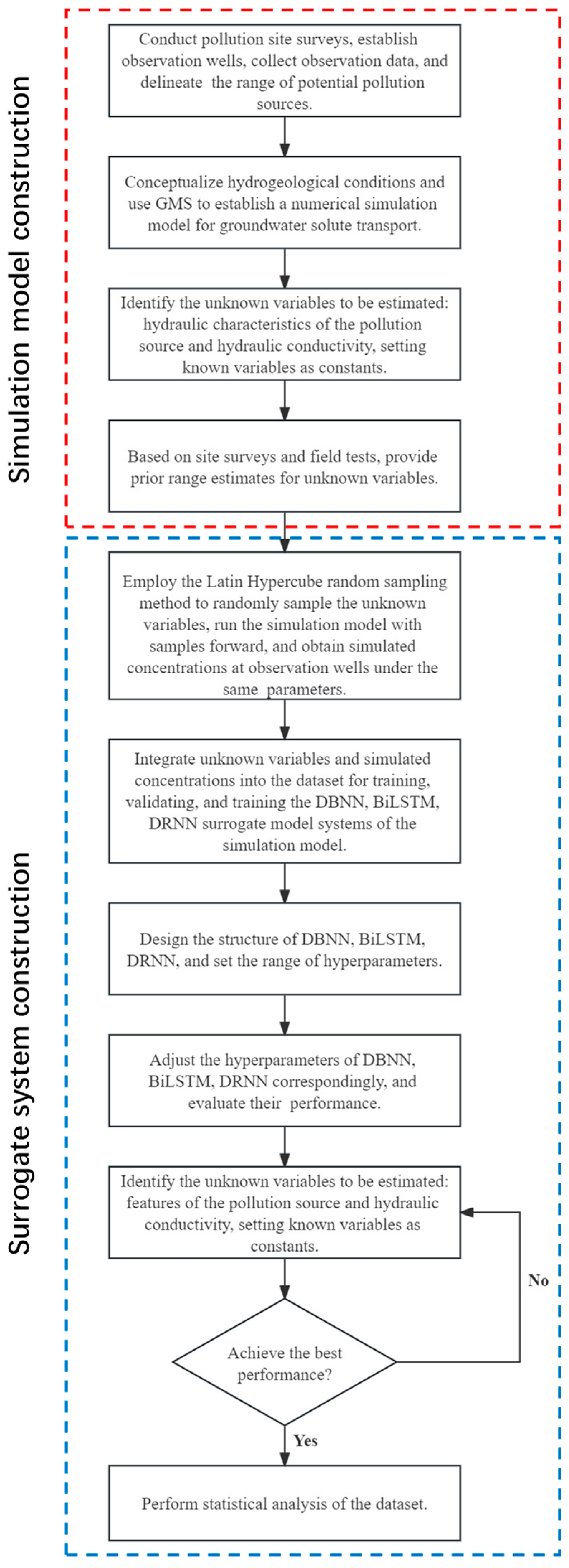
2. Methodology and Theory

2.1. Multiphase Flow Numerical Simulation Model

In this study, we use a two-dimensional (2D) heterogeneous isotropic groundwater system simulation model, which includes both groundwater flow and solute transport models. The groundwater flow numerical simulation model describes the entire process of groundwater flow and solute transport. In this study, the groundwater flow is governed by the following equations [40]. In the formula, where Kij is the hydraulic conductivity, H is the hydraulic head, W is the volumetric flux per unit volume, μ is the specific yield, Γ is the boundary of the simulation domain, and x and y are the Cartesian coordinates.

$${\displaystyle \frac{\partial }{\partial x_i}}\left(K_{ij}{\displaystyle \frac{\partial H}{\partial x_j}}\right)+W=\mu {\displaystyle \frac{\partial H}{\partial t}}\left(x,y\right)\in \Gamma i,j=1,2\mathrm{t}\ge 0$$

(1)

Combining the groundwater flow numerical equations, the solute transport can be described by the following formula:

$${\displaystyle \frac{\partial C}{\partial t}}={\displaystyle \frac{\partial }{\partial x_i}}\left(D_{ij}{\displaystyle \frac{\partial C}{\partial x_j}}\right)-{\displaystyle \frac{\partial }{\partial x_i}}\left(u_{ij}C\right)+{\displaystyle \frac{R}{\theta }}\left(x,y\right)\in \Gamma i,j=1,2t\ge 0$$

(2)

$$u_i={\displaystyle \frac{K_{ij}}{\theta }}{\displaystyle \frac{\partial H}{\partial x_i}}i,j=1,2$$

(3)

where t stands for the time, C stands for the contamination concentration, $D_{ij}$ stands for the dispersion coefficient, $u_{ij}$ stands for the linear velocity of the groundwater flow following Darcy’s Law, $u_i$ stands for average velocity, R is the source or sink term, θ is the effective porosity of the aquifer medium, and Γ is the boundary of the simulation domain. On the basis of the numeric simulation equation, the groundwater flow and solute transport simulation model was established by employing the MODFLOW module and MT3D module in groundwater modeling systems (GMS).

2.2. Surrogate Model

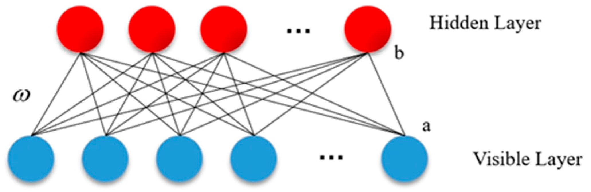
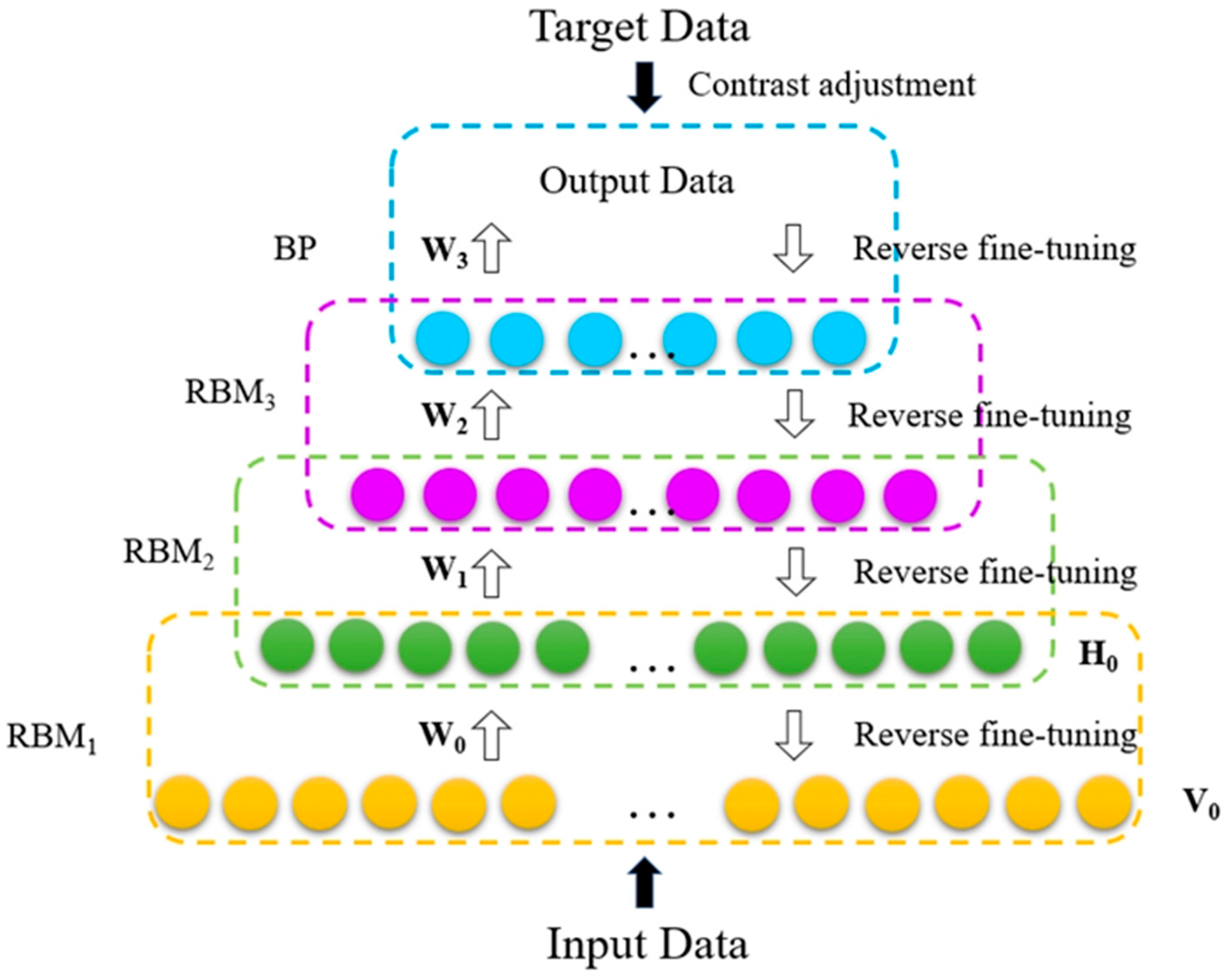
2.2.1. The DBNN Method

The DBNN is a popular deep-learning model that has been widely applied in multiple fields since its inception. The training process of a DBNN consists of two main stages: first, an unsupervised pre-training phase, followed by a supervised fine-tuning phase. This structure allows the DBNN to effectively learn and extract multi-level feature representations from data [41].

The architecture of DBNN includes multiple layers of RBM. The schematic diagram of an RBM is shown in Figure 2, where the upper red neurons form the hidden layer and the blue neurons form the visible layer. These layers are connected in series to form a multi-layer network, thereby learning the data’s distribution and complex feature representations. Specifically, DBNN consists of an input layer, several hidden layers (each composed of an RBM), and an output layer, as illustrated in Figure 3. Each RBM comprises a visible layer and a hidden layer, with layers connected by weights that are responsible for transmitting and transforming data information, thus achieving the extraction of features from simple to complex.

This hierarchical learning method not only improves learning efficiency but also enhances the model’s fitting ability, making DBNN perform exceptionally well in handling complex data problems. The output layer algorithm is used to predict the output results, and in this study, the Backpropagation (BP) neural network algorithm is chosen as the top-level algorithm.

During the training process of RBM, the energy function is a core concept used to define the probability distribution of network states. Inspired by the Boltzmann distribution from statistical physics, this function aims to measure the “energy” or “cost” of specific states. The lower the energy, the higher the stability of the state, and the greater its probability of occurrence. In this way, RBM uses the energy function to represent the likelihood of different network states, thereby guiding the network to reduce the total system energy through learning, enhancing the accuracy and efficiency of data representation [42]. This makes RBM particularly suitable for extracting features and discovering hidden structures in data in an unsupervised learning context [43].

• The unsupervised learning training stage.

First, the RBM is trained layer-by-layer from the bottom up to extract the fundamental content of the input data. The joint probability distribution for one set of states, referred to as $(v,h)$, is as follows.

$$P(v,h;\theta )={\displaystyle \frac{e^{-E(v,h;\theta )}}{Z(\theta )}}$$

(4)

In this context, $P\left(v,h;\theta \right)$ represents the joint probability distribution of the visible units $v$ and hidden units $h$ occurring simultaneously, given the parameters $\theta$. It is determined by the energy function $E(v,h;\theta )$ and the normalization constant $Z\left(\theta \right)$, with $E(v,h;\theta )$ and $Z\left(\theta \right)$ defined as follows:

$$E(v,h;\theta )=-({\displaystyle \sum _{i=1}^n{a}_i{v}_i+{\displaystyle \sum _{j=1}^m{b}_j{h}_j+{\displaystyle \sum _{i=1}^n{\displaystyle \sum _{j=1}^m{\omega }_{ij}{v}_i{h}_j}}}})$$

(5)

$$Z(\theta )={\displaystyle \sum _v{\displaystyle \sum _h{e}^{-E(v,h;\theta )}}}$$

(6)

where $V={\left\{v_i\right\}}_{i=1}^n$ stands for the neurons in the visible layer of the RBM, $n$ stands for the number of neurons in the visible layer. $H={\left\{h_j\right\}}_{j=1}^m$ stand for the neurons in the hidden layer of the RBM, m stands for the number of neurons in the hidden layer. $\theta =\left\{\omega ,a,b\right\}$ stands for the vector of bias parameters in the RBM. $A={\left\{a_i\right\}}_{i=1}^n$ stands for the biases of the neurons in the visible layer, $B={\left\{b_j\right\}}_{j=1}^m$ stands for the biases of the neurons in the hidden layer. $P\left(v,h;\theta \right)$ stands for the joint probability distribution of the visible layer parameters $v$ and hidden layer parameters $h$ given the parameters $\theta$. $Z\left(\theta \right)$ stands for the normalization constant that ensures $P\left(v,h;\theta \right)$ is a valid probability distribution. ${\omega }_{ij}$ stands for the connection weights between the visible layer and the hidden layer.

In DBNN, particularly during the RBM stages, one of the core tasks is to adjust the model’s parameters to maximize the likelihood function. This process involves finding a set of model parameters that best explain the observed data. The energy function plays a key role here as it defines the probabilities and statistical weights of various states in the network. By minimizing this energy function, we not only aim to find parameters that optimize model performance but also strive to maintain the appropriate generalization ability of the model, avoiding overfitting.

During the unsupervised learning phase of DBNN, the log-likelihood function becomes a crucial tool that helps the model learn useful features hidden within the data. These features effectively capture the important statistical regularities of the input data, laying a solid foundation for the subsequent supervised learning phase. Specifically, the log-likelihood function measures the efficiency with which a given set of parameters (including weights and biases) can generate the observed data, which also reflects the model’s capability in describing the data.

By continuously adjusting these parameters and optimizing the log-likelihood function, the DBNN can learn and represent data features more accurately, thereby improving its prediction and classification accuracy on multiple levels. We optimized the DBNN model by maximizing the log-likelihood function. The purpose of this optimization process is to enable the model to better fit the training data and more accurately capture the data’s characteristics. Maximizing the log-likelihood function can enhance the model’s generalization ability, allowing it to better adapt to different types of data distributions; this optimization provides foundational support for the potential effectiveness of the DBNN model in practical applications [44]. The logarithm of the likelihood function is given by:

$$L\left(\theta \right)={\displaystyle \sum _{i=1}^l\ln P\left(v_i,h\right)}$$

(7)

$$\ln P(v,h)=\ln [{\displaystyle \frac{1}{Z(\theta )}}{\displaystyle \sum _{j=1}^m\exp (-E(v,h;\theta )}]$$

(8)

where $l$ stands for the total number of input samples.

During the training process of RBM, the Contrastive Divergence (CD) method is commonly used to update weights as well as biases in the visible and hidden layers in order to accelerate training and effectively approximate the global gradient. This method is implemented through a specific sampling technique designed to approximate the summation process over the entire data space, thereby enhancing the overall training efficiency.

The CD algorithm works through the following steps: First, a sample is drawn from the dataset, and its activation state in the visible layer is calculated; next, based on this state, a hidden layer state is generated using the model’s current parameters; then, the visible layer state is regenerated using these hidden layer states; finally, a new hidden layer state is generated based on the updated visible layer state. This process of moving from the visible layer to the hidden layer and back to the visible layer is typically repeated several times (this repetition number is referred to as the “step size” of CD) and is used to update the model’s weights and biases.

This method effectively balances computational efficiency and training quality. By conducting a limited number of state reconstructions, CD can rapidly and approximately simulate the complete probability distribution process, thereby speeding up convergence and reducing the computational burden. This enables RBM to achieve convergence more quickly while maintaining the efficiency and accuracy of model training.

The formula for the Contrastive Divergence algorithm is as follows:

$$\Delta {\omega }_{ij}=\eta \left[{(v_i{h}_j)}_{data}-{\left(v_i{h}_j\right)}_{recon}\right]$$

(9)

$$\Delta a_i=\eta \left[{(v_i)}_{data}-{\left(v_i\right)}_{recon}\right]$$

(10)

$$\Delta b_j=\eta \left[{(h_j)}_{data}-{\left(h_j\right)}_{recon}\right]$$

(11)

where $\eta$ stands for the learning rate, ${(\cdot )}_{data}$ stands for the expected value based on the actual data, ${(\cdot )}_{recon}$ stands for the expected value based on the reconstructed data. $\Delta {\omega }_{ij}$ stands for the update applied to the weight ${\omega }_{ij}$ connecting the $i$th visible neuron and the $j$th hidden neuron. $\Delta a_i$ stands for the update amount for the bias $a_i$ of the $i$th neuron in the visible layer, and $\Delta b_j$ stands for the update amount for the bias $b_j$ of the $j$th neuron in the hidden layer. ${\left(v_i{h}_j\right)}_{data}$ stands for the expected value of the visible layer neurons $v_i$ and hidden layer neurons $h_j$ being activated simultaneously under the data distribution, calculated directly from the training data. ${\left(v_i{h}_j\right)}_{recon}$ stands for the expected value of the visible layer neurons $v_i$ and hidden layer neurons $h_j$ being activated simultaneously under the reconstruction distribution, typically obtained through calculations from the training data. ${\left(v_i\right)}_{data}$ stands for the expected value of neuron $v_i$ in the visible layer under the data distribution, while ${\left(v_i\right)}_{recon}$ stands for the expected value of neuron $v_i$ in the visible layer under the reconstruction distribution. ${\left(h_j\right)}_{data}$ stands for the expected value of neuron $h_j$ in the hidden layer under the data distribution, and ${\left(h_j\right)}_{recon}$ stands for the expected value of neuron $h_j$ in the hidden layer under the reconstruction distribution.

2.

The supervised learning training stage.

After the RBM completes its unsupervised pre-training, the next step is the supervised learning training stage, which is the second crucial phase in the DBNN training process. In this stage, it is vital to continuously fine-tune the network structure to enhance its performance.

The specific formula for parameter updates is as follows: ${\omega }_{ij}$ stands for the weight update term, $b_j$ stands for the parameter update term for the bias items in the DBNN, $\eta$ stands for the learning rate, and $E{r}_j$ refers to the loss function.

$${\omega }_{ij}={\omega }_{ij}-\eta {\displaystyle \frac{\partial E{r}_j}{\partial {\omega }_{ij}}}$$

(12)

$$b_j=b_j-\eta {\displaystyle \frac{\partial E{r}_j}{\partial b_j}}$$

(13)

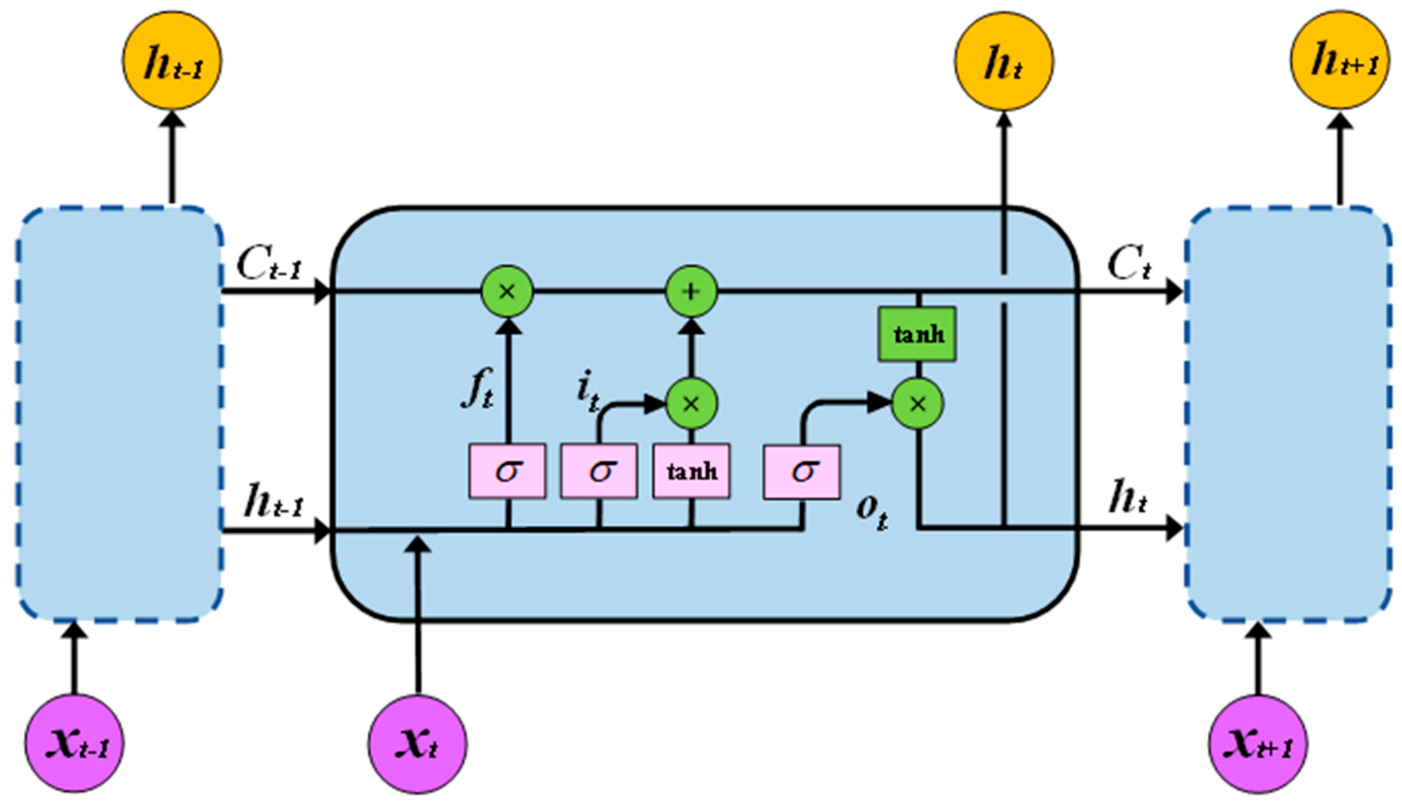
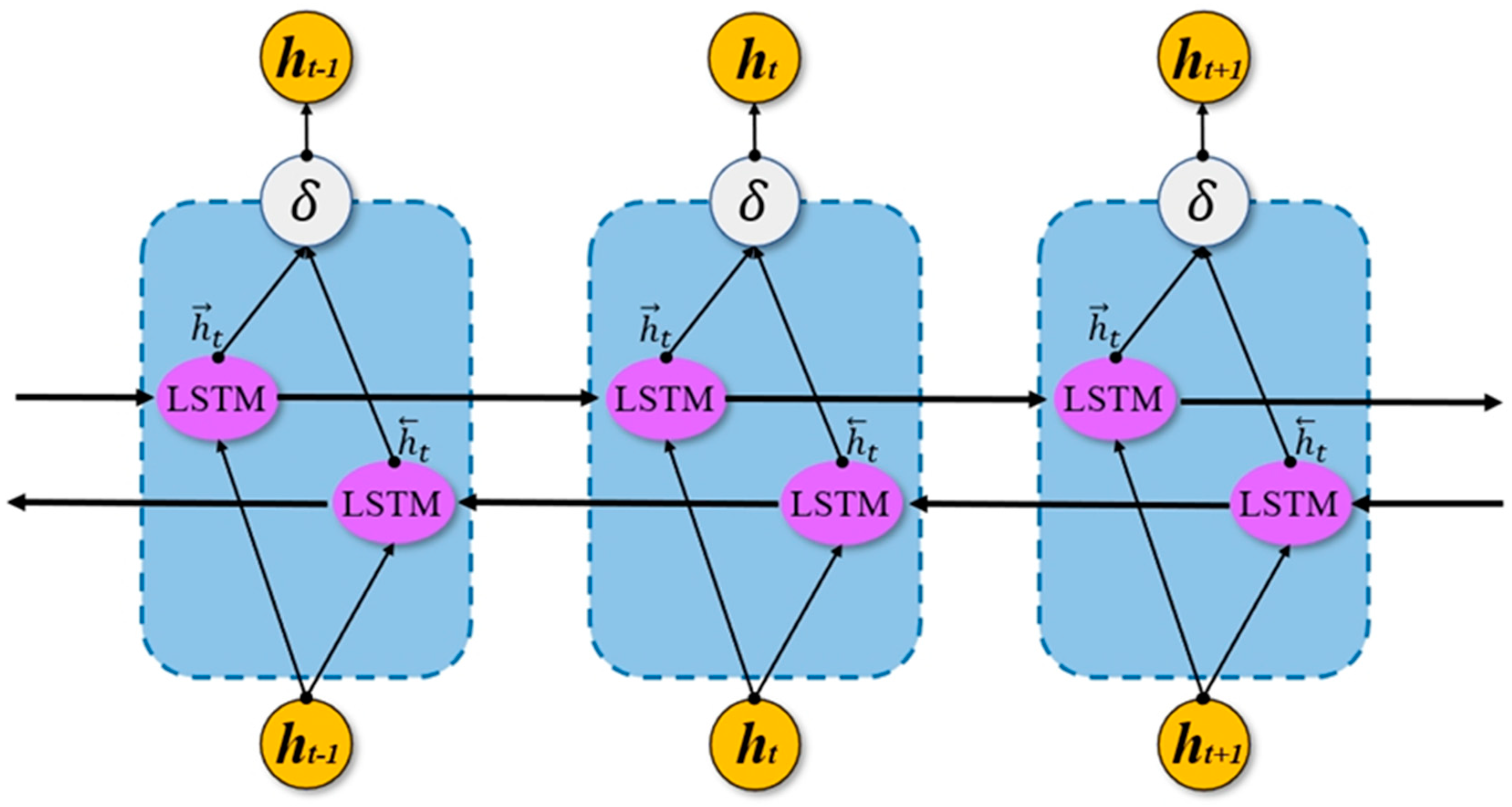
2.2.2. The BiLSTM Method

The BiLSTM is a variant of the LSTM, which belongs to the special family of RNN. LSTM was specifically designed to address the issues of vanishing and exploding gradients that traditional RNN face when processing long sequence data. By incorporating “memory blocks,” LSTM is able to effectively preserve information over long sequences. These memory blocks consist of three main components: the input gate, the forget gate, and the output gate. They work together to control the preservation, updating, and deletion of information, thereby maintaining the network’s long-term memory characteristics and providing a forward propagation chain structure [45], as shown in Figure 4.

The LSTM has three inputs, i.e., the $(t-1)$-th hidden state $h_{t-1}$, the $(t-1)$-th unit state $C_{t-1}$, and the $t$-th heart rate data. The outputs of LSTM are the $t$-th unit state Ct and the $t$-th hidden state $h_t$.

LSTM have three “gates” that determine the rate at which information is processed. The formulas are as follows:

1. In Formula (14), the forget gate $f_t$ uses the cell state $C_{t-1}$ from the previous time step (t − 1) to discard irrelevant information and retain essential information.

2. In Formula (15), the input gate, shown here, is used to extract relevant information, and then input it into the network.

3. The output gate $o_t$, as shown in Formula (16), is used to obtain the output $h_t$. ${\tilde{C}}_t$ represents the candidate state, as shown in Formula (17). The cell state $C_t$ is represented as shown in Formula (18), and the hidden state $h_t$, as shown in Formula (19). $\sigma \left(·\right)$ represents the sigmoid activation function for this model, as shown in Formula (20), and $\tanh \left(·\right)$ stands for the tanh activation function. When $\sigma$ = 0, the data will pass through the output gate $o_t$; conversely, it will not be able to pass through this gate. The circles in the diagram represent the rules for operations between vectors. $\otimes$ stands for Hadamard Product, and $\oplus$ stands for Direct Sum.

In Figure 4, the values $h_{t-1}$ and $x_t$ are used to calculate the outputs of all gates $o_t$ and the candidate state ${\tilde{C}}_t$, where $W_f$ is the weight connecting the input layer to the forget gate, $W_i$ is the weight connecting the input layer to the input gate, $W_o$ is the weight connecting the input layer to the output gate, and $W_c$ is the weight connecting the input layer to the candidate state ${\tilde{C}}_t$. $U_f$ is the weight connecting the hidden state $h_{t-1}$ to the forget gate, $U_i$ is the weight connecting the hidden state $h_{t-1}$ to the input gate, $U_o$ is the weight connecting the hidden state $h_{t-1}$ to the output gate, and $U_c$ is the weight connecting the hidden state $h_{t-1}$ to the candidate state ${\tilde{C}}_t$. The hidden state at timestep $t$-th, $h_t$, is calculated using Formulas (14)–(20), which also serve as the output of the LSTM.

$$f_t=\sigma \left(W_f{x}_t+U_f{h}_{t-1}+b_f\right)$$

(14)

$$i_t=\sigma \left(W_i{x}_t+U_i{h}_{t-1}+b_i\right)$$

(15)

$$o_t=\sigma \left(W_o{x}_t+U_o{h}_{t-1}+b_o\right)$$

(16)

$${\tilde{C}}_t=\tanh \left(W_c{x}_t+U_c{h}_{t-1}+b_c\right)$$

(17)

$$C_t=f_t\cdot C_{t-1}+i_t\cdot {\tilde{C}}_t$$

(18)

$$h_t=o_t\cdot \tanh \left(C_t\right)$$

(19)

$$\sigma \left(x\right)={\displaystyle \frac{1}{1+e^{-x}}}$$

(20)

The expression for $\tanh \left(\cdot \right)$ is as follows:

$$\tanh \left(x\right)={\displaystyle \frac{e^x-e^{-x}}{e^x+e^{-x}}}$$

(21)

BiLSTM is an improved structure of LSTM, as shown in Figure 5 and in its schematic diagram, $\delta$ stands for the connection function that links the forward and backward inputs. BiLSTM includes a forward LSTM layer and a backward LSTM layer. This structure, by considering both the preceding and following contexts of information simultaneously, allows BiLSTM to comprehensively analyze both historical and future data. In these two layers, the forward LSTM processes data in chronological order, producing the sequence: ${\overrightarrow{h}}_i=\left\{h_1,h_2,\dots ,h_t\right\}$. Its processing method is the same as traditional LSTM. Backward LSTM Layer: This layer processes data in reverse order of time to obtain a sequence ${\overleftarrow{h}}_i=\left\{h_t,h_{t-1},\dots ,h_1\right\}$ to incorporate future information while processing data at each time point.

By introducing “memory blocks”, LSTM is equipped with a chain structure that allows for the forward transmission of information. BiLSTM further extends this capability with its bidirectional structure, not only maintaining the forward information flow but also incorporating a reverse information transmission chain. This greatly enhances the model’s ability to handle sequential data and its flexibility. Therefore, BiLSTM is particularly suited for tasks that require consideration of bidirectional context, enabling simultaneous analyses of both past and future information.

The output of BiLSTM is represented as: ${\overleftrightarrow{h}}_i$.

$${\overleftrightarrow{h}}_i=\delta \left({\overrightarrow{h}}_i,{\overleftarrow{h}}_i\right)$$

(22)

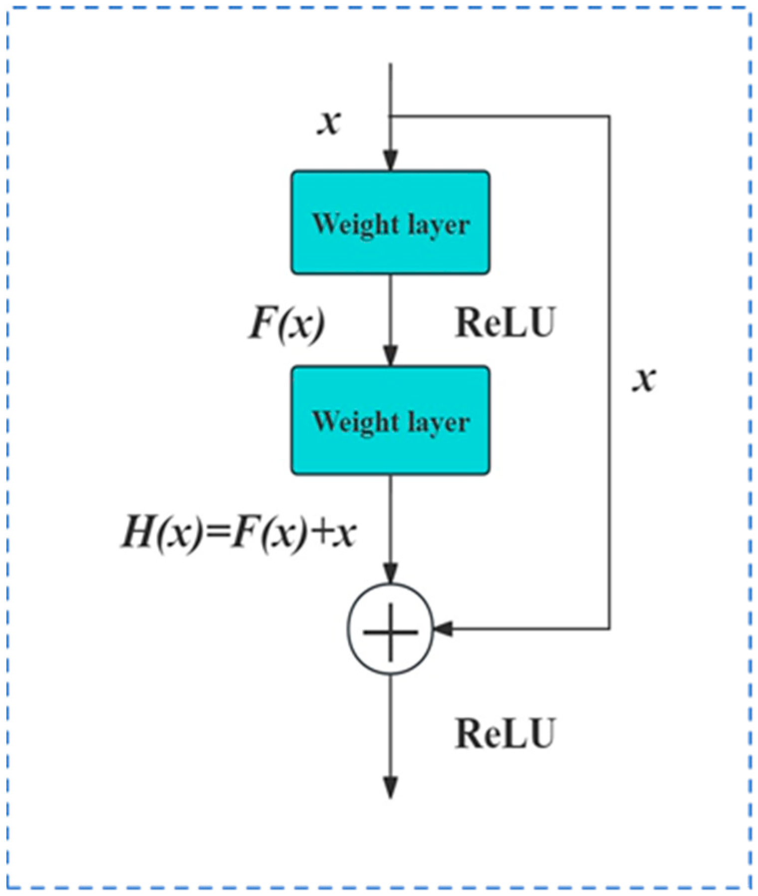
2.2.3. The DRNN Method

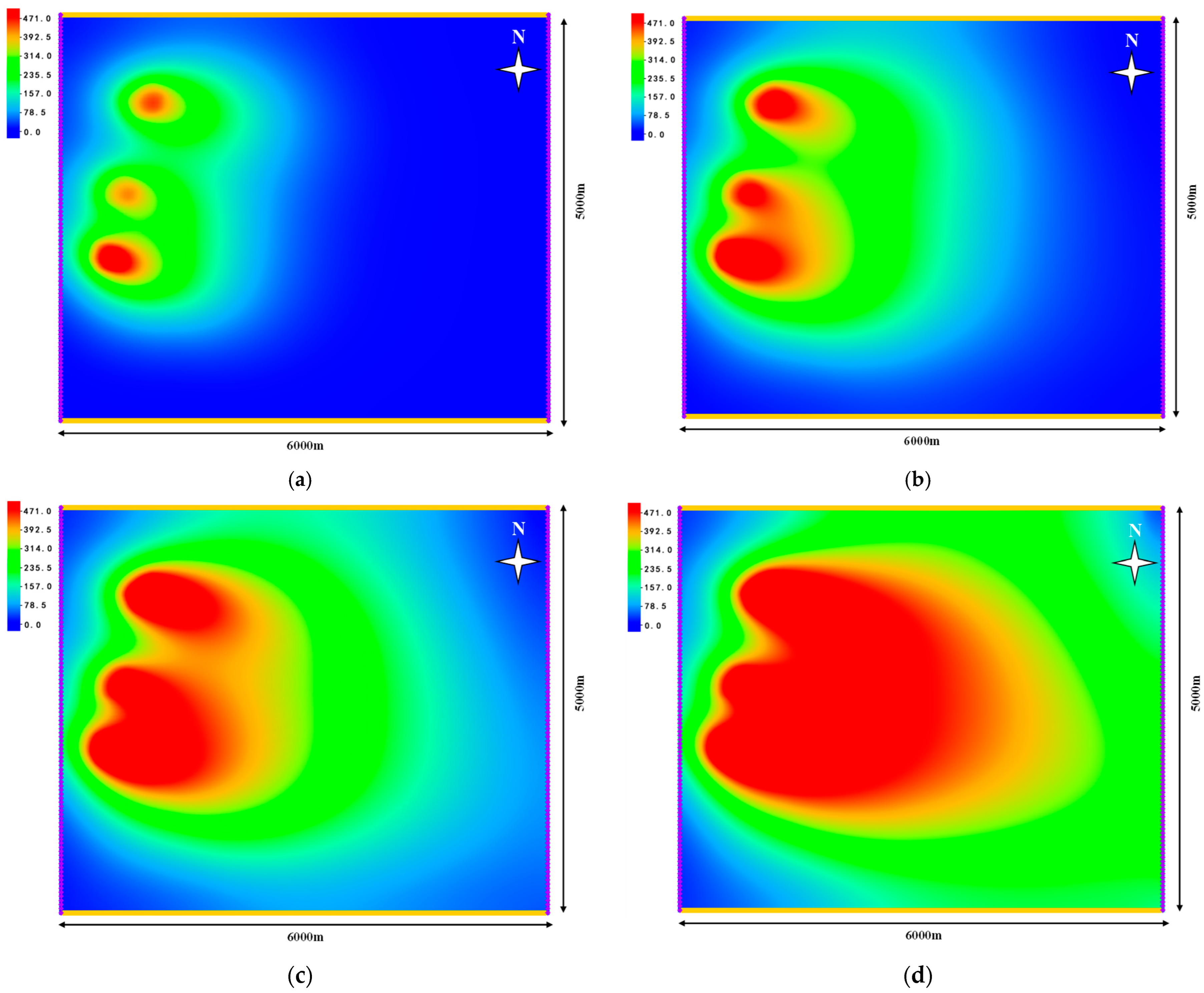
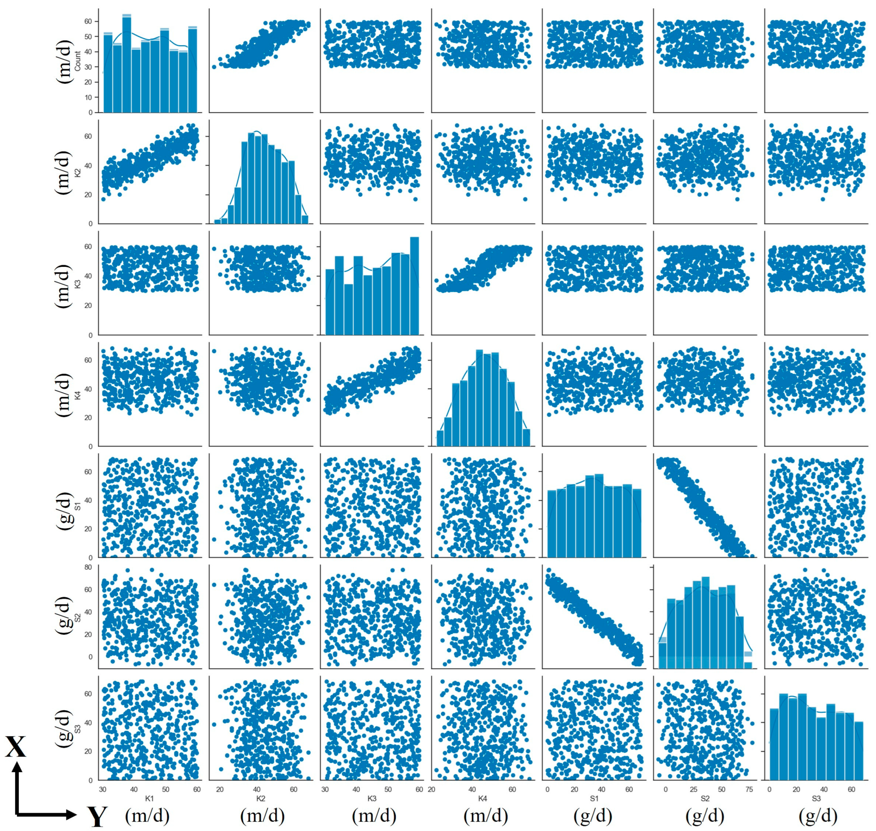
In RNN, as the number of time steps increases, the gradients in the backpropagation process may rapidly increase (gradient explosion) or decrease (gradient vanishing). This phenomenon leads to deficient performance when the model processes sequences with varying lengths or complex dependencies. To address these issues, He et al. proposed the concept of Residual Networks (ResNet). This concept was later applied to improve the structure of DRNN by introducing residual connections, which help alleviate the problem of vanishing gradients and thus enhance the model’s ability to handle long sequence data [46].

Compared to traditional neural networks, the core feature of DRNN built on the ResNet concept is the adoption of “residual learning.” Each residual block within a DRNN typically includes two or more convolutional layers, and features skip connections between the input and output of these layers. These skip connections allow gradients to directly pass through some layers. This architectural design significantly enhances gradient stability and learning efficiency when processing sequential data, as it helps to prevent the issue of gradient vanishing, thereby enabling the training of deeper networks. Unlike the ordinary neural network, the core of ResNet is the residual block (ResBlock) (Figure 6).

Introducing the concept of residual learning from ResNet into DRNN effectively addresses the problems of gradient explosion and vanishing that traditional RNNs encounter. This improvement significantly enhances the model’s performance in handling data with complex dependencies and long sequences. The structure of DRNN not only increases the depth of network training but also improves the efficiency of information transmission and gradient flow. As a result, DRNN have demonstrated outstanding performance in a variety of sequence processing tasks, including language processing and time series analysis, proving their broad application potential and practical value.

In ResNet, the learning objective is to map the relationship between the input and the residuals: $F\left(x\right)=H\left(x\right)-x$, rather than directly learning the target mapping $H\left(x\right)$ at each layer. Here, $F\left(x\right)$ represents the residual mapping function, $x$ represents the input, and $H\left(x\right)$ represents the target mapping function that needs to be learned, with $\oplus$ representing the Direct Sum. This structure makes it easier for the network to learn mapping relationships, aids in the transmission of information throughout the network, mitigates the problem of vanishing gradients, and enhances both the efficiency and effectiveness of training.

In ResNet, the actual residual mapping can be represented as:

$$F(x)=W_2\sigma \left(BN\left(W_1\sigma \left(BN\left(x\right)\right)\right)\right)$$

(23)

In this context, $W_i$ represents the weight matrix of the convolutional layer, $\sigma \left(·\right)$ denotes the activation function, $BN$ stands for batch normalization, and $F\left(x\right)$ represents the final residual mapping function.

The overall computation formula for the residual block is expressed as:

$$Output=\sigma (F(x)+x)$$

(24)

In this context, $F\left(·\right)$ is the residual function and $x$ is the input. The direct transmission of $x$ ensures that, even in networks with many layers, input information can effectively propagate to deeper layers, helping to maintain the integrity of the information and facilitate normal gradient flow. $\sigma$ stands for the activation function, which performs a nonlinear transformation on the result of $F\left(x\right)+x$. $Output$ is the final output, which will be passed on to the next layer of the network. This section describes the construction of a DRNN model using the ResNet residual network.

3. Case Description

This article is based on a case study of no-point source pollution designed around the actual pollution incidents in the Songhua River Basin in Harbin, Heilongjiang Province, China. The study area covers 30 km², with the terrain being higher in the northwest and lower in the east and west, and the groundwater flow direction is from northwest to southeast. The research area is conceptualized as a heterogeneous isotropic aquifer, and the study subject is an unconfined aquifer with a two-dimensional steady flow. As shown in Figure 7, the yellow boundary represents a no-flow boundary, and the purple boundary represents a specified head boundary.

In the conceptual model, groundwater flow is assumed to comply with Darcy’s Law, meaning that the flow velocity is proportional to the hydraulic gradient, and the assumption of isotropy within the system allows us to simplify the calculations by assuming that hydraulic conductivity is the same in all directions. This assumption is particularly important in a two-dimensional model, as it simplifies the complex three-dimensional flow problem into a two-dimensional one, making it easier to perform numerical simulations using the MODFLOW and MT3D modules.

The aquifer in the study area can be divided into four different hydraulic conductivity zones based on its yield: K1, K2, K3, and K4. The river boundaries on the west and east are conceptualized as specific head boundaries. Due to the granite in the north and south, which has poor permeability, these boundaries are conceptualized as no-flow boundaries.

Table 1. Basic values and ranges of contamination sources and aquifer.

Parameter	Value/Range
Hydraulic conductivity (m/day)	(30, 60)
Specific yield	0.22
Saturated thickness (m)	50
Longitudinal dispersivity	45
Transverse dispersivity	19.6
Grid spacing in x-direction (m)	10
Grid spacing in y-direction (m)	10
Stress periods (year)	5
Fluxes of contamination source during stress period (g/day)	(0, 69)

details the basic values and ranges of the aquifer and pollution sources. The area contains three pollution sources, all of which are non-point sources. The pollution discharge history is divided into five years, with each year representing a period totaling five periods. The study area is spatially discretized into units of 100 m × 100 m. To monitor pollutants more accurately, six monitoring wells are set up, including obs1, obs2...obs6.

Table 2. Reference values of unknown variables to identify.

Unknown Variables to Identify	Reference Value
Fluxes of pollution source, S1T1 (g/d)	36
Fluxes of pollution source, S1T2 (g/d)	41
Fluxes of pollution source, S1T3 (g/d)	55
Fluxes of pollution source, S1T4 (g/d)	60
Fluxes of pollution source, S1T5 (g/d)	59
Fluxes of pollution source, S2T1 (g/d)	28
Fluxes of pollution source, S2T2 (g/d)	30
Fluxes of pollution source, S2T3 (g/d)	34
Fluxes of pollution source, S2T4 (g/d)	36
Fluxes of pollution source, S2T5 (g/d)	35
Fluxes of pollution source, S3T1 (g/d)	46
Fluxes of pollution source, S3T2 (g/d)	51
Fluxes of pollution source, S3T3 (g/d)	58
Fluxes of pollution source, S3T4 (g/d)	56
Fluxes of pollution source, S3T5 (g/d)	62
Hydraulic conductivity in partition, k1(m/d)	41.1
Hydraulic conductivity in partition, k1(m/d)	55.7
Hydraulic conductivity in partition, k1(m/d)	50.2
Hydraulic conductivity in partition, k1(m/d)	52.9

lists the true reference values for the unknown variables to be identified, totaling 19 variables, including four different hydraulic conductivity areas: K = K1, K2, K3, and K4. The release history of the three pollution sources, SaTb (a = 1, 2, 3; b = 1, 2, 3, 4, 5), where SaTb represents the intensity of pollution source a during period b.

In this study, a hypothetical case was set up based on real-world conditions of no-point source pollution. Therefore, the true values of the variables to be identified were input into the simulation model, which was then run to obtain the pollutant concentration data at each period from the observation wells. These simulated observations were subsequently compared with the actual observed values. Figure 8 shows the distribution of groundwater pollutant solute transport.

In this study, there are six monitoring wells in the research area, with a simulation period of five years. Each well undergoes a monitoring cycle of one year, resulting in continuous monitoring over five years. Therefore, each set of data on pollutant concentration monitoring includes 30 pollutant concentration measurements. In the surrogate model, training data are used to extract fixed features and patterns from the simulation model, while validation data are used to assess the generalization ability of the surrogate model.

The accuracy of the approximation is evaluated using three standard metrics: Mean Absolute Error (MAE), Root Mean Square Error (RMSE), and the coefficient of determination R².

$$RMSE=\sqrt{{\displaystyle \frac{1}{n}}{\displaystyle \sum _{i=1}^n{\left(y_i^b-y_i^q\right)}^2}}$$

(25)

$$R^2=1-{\displaystyle \sum _{i=1}^n\frac{{\left(y_i^b-y_i^q\right)}^2}{{\left(y_i^b-m^b\right)}^2}},m^b={\displaystyle \frac{1}{n}}{\displaystyle \sum _{i=1}^n{y}_i^b}$$

(26)

$$M\mathrm{A}E={\displaystyle \frac{1}{n}}{\displaystyle \sum _{i=1}^n\left|y_i^b-y_i^q\right|}$$

(27)

In the formular, $y_i^b$ represents the output samples from the numerical simulation model, $y_i^q$ represents the output samples from the surrogate simulation model, and n denotes the number of samples in the model.

In this study, surrogate models are constructed using DBNN, BiLSTM, and DRNN. These models are evaluated using training and validation datasets. The performance of the surrogate model system is assessed based on time cost and approximation accuracy. The time cost is estimated by measuring the duration required for the same number of iterations, with calculations performed on a PC equipped with an Intel Core i5-1135G7 @ 2.40 GHz processor and 16 GB RAM (Intel Co. Ltd., Santa Clara, CA, USA).

4. Results and Discussion

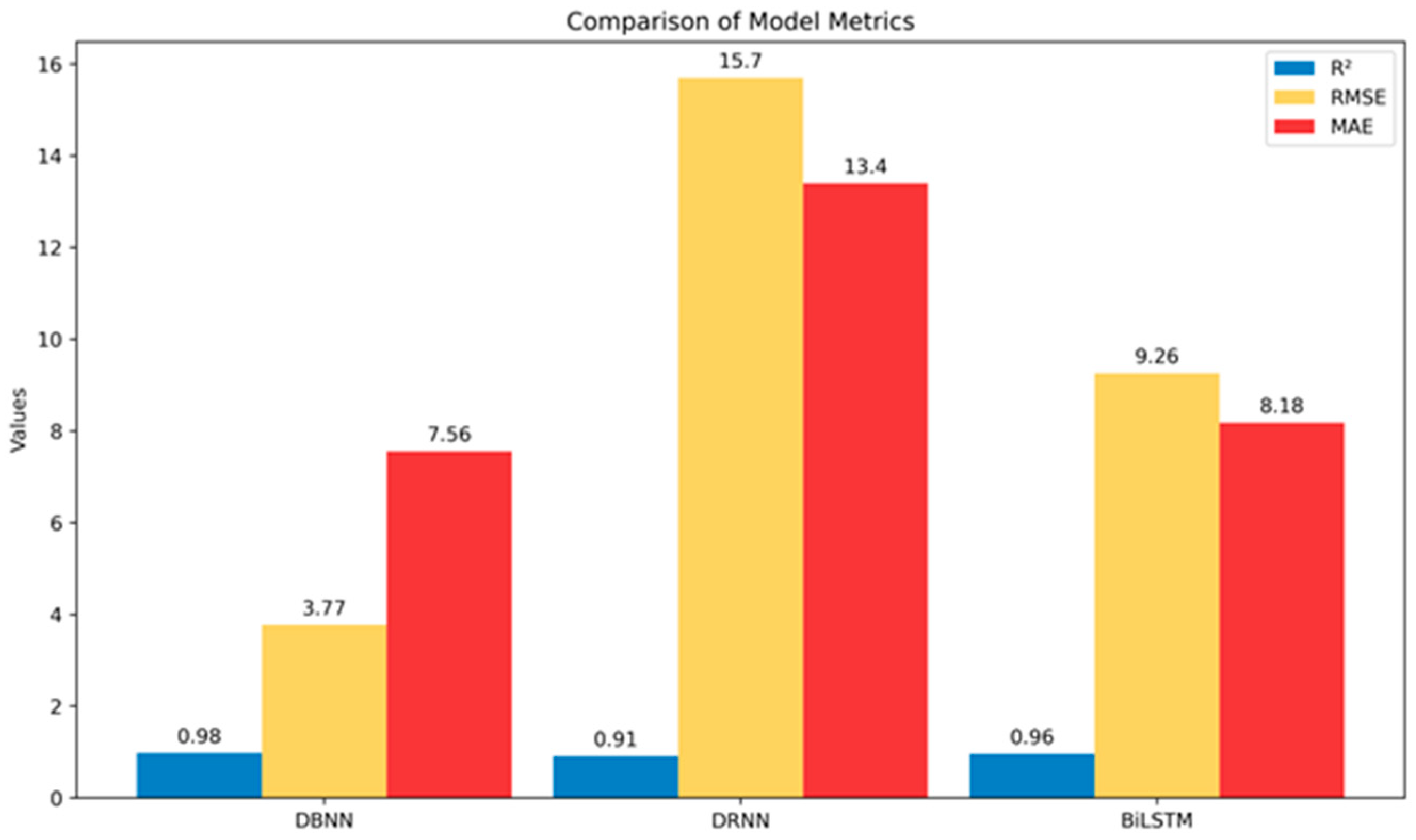
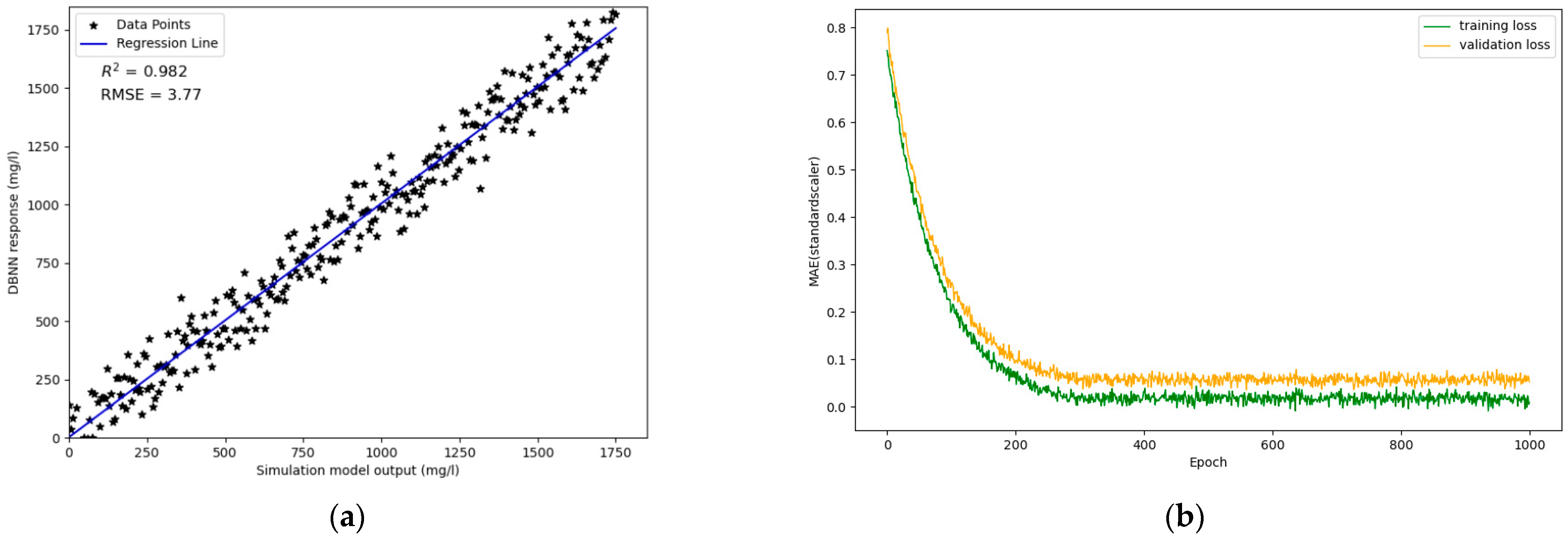
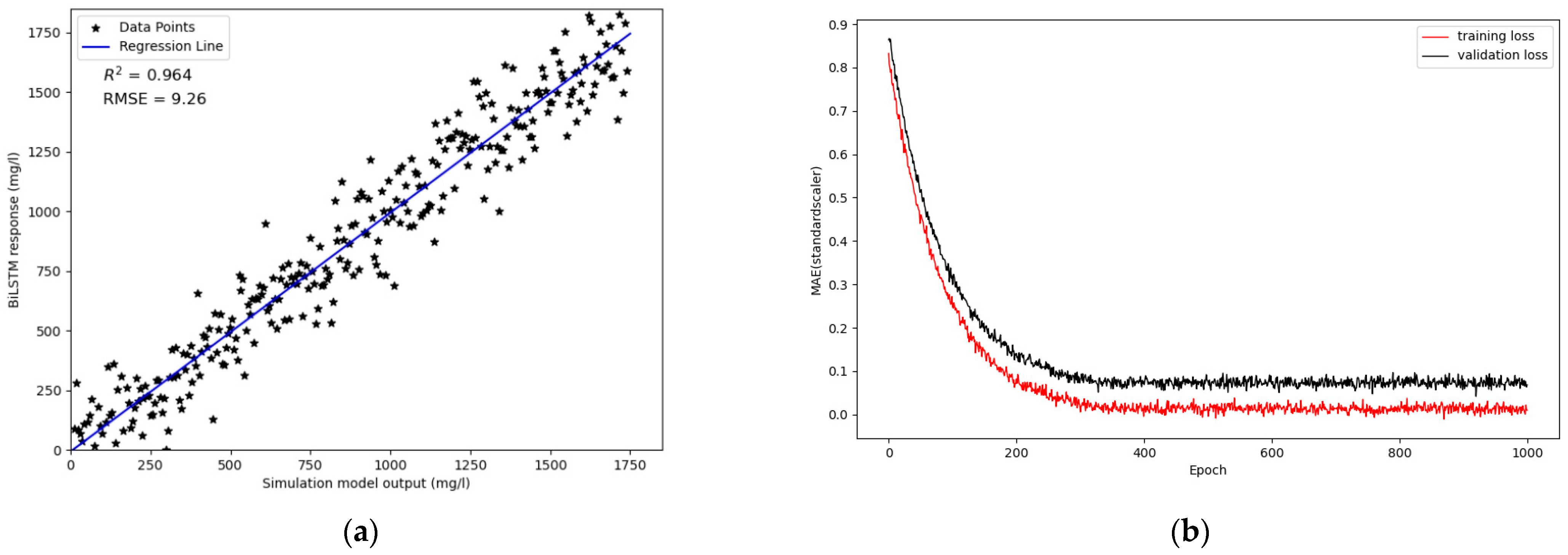
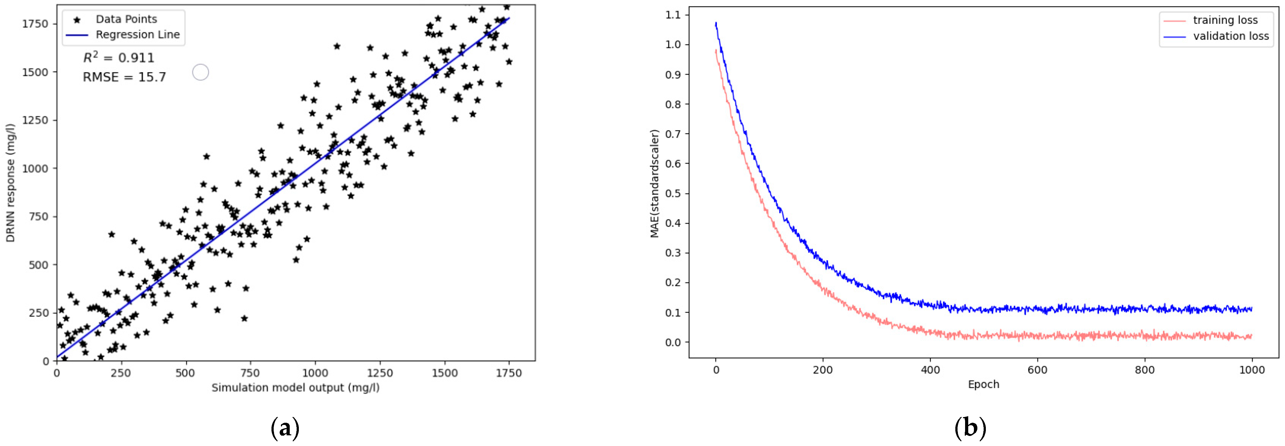
4.1. Performance of Surrogate System

In this case study, we utilized and compared three surrogate models: DBNN, BiLSTM, and DRNN. All mentioned surrogate models were computed using 2000 dataset samples. To ensure uniform coverage across the sampling interval and enhance the representativeness of the samples, Latin Hypercube Sampling (LHS) was employed to sample the values of hydraulic conductivity K (K1, K2, K3, and K4) and the pollutant release intensities SaTb (a = 1, 2, 3; b = 1, 2, 3, 4, 5). This process generated 2000 random combinations of hydraulic conductivity and pollutant release intensities for different periods, selecting and randomly combining these parameters into 2000 sets. Figure 9 displays the multivariate joint distribution diagram obtained through LHS, where the variables exhibit a normal distribution, with exceptions such as K1 and K4, which show a distinct multimodal distribution. The scatter plots on the off-diagonals illustrate the correlations between variables.

Subsequently, the 19-dimensional data extracted via the LHS method was input into the groundwater solute transport simulation model. Utilizing the GMS software (10.7), we generated output sample datasets of pollutant concentrations as detected by 2000 sets of monitoring wells. This process yielded a total of 2000 pairs of sample input and output datasets. These datasets were then divided into a training dataset comprising 1400 sets (70%) and a validation dataset consisting of 600 sets (30%). The 2000 dataset sets were subsequently processed using the three surrogate models: DBNN, BiLSTM, and DRNN.

To visualize the performance of the surrogate models, we plotted comparison graphs of the R², MAE, and RMSE responses for each model in Figure 10. The performance charts reveal that, compared to the BiLSTM and DRNN methods, the DBNN demonstrated higher R² values and lower RMSE and MAE. This indicates that the DBNN method exhibits superior performance characteristics in constructing surrogate models for complex, high-dimensional nonlinear inverse problems, particularly in handling non-point source pollution data.

Further comparison of the DBNN method’s performance is evident in Figure 10, which shows that DBNN achieved a higher R² and lower RMSE. This indicates that the initial unsupervised pre-training step used to initialize the network weights, coupled with the subsequent supervised learning training phase, significantly enhanced the accuracy of the validation. This approach has effectively alleviated the issue of overfitting to some extent.

Figure 11, Figure 12 and Figure 13 display the fitting results of the three methods compared to the actual values. We extracted 300 sets of data from the simulation dataset to display as samples in the graph. Figure 11a,b show the training curve of the DBNN, which clearly converges after undergoing 300 training iterations. It presents a comparison between the DBNN predicted values and the training model’s output values. An R² value of 0.982 indicates that the DBNN surrogate model approximates the true values very well and can simulate the model with high precision.

Figure 12a,b display the training curve of the BiLSTM, which shows convergence after approximately 390 training iterations. It illustrates a comparison between the BiLSTM predicted values and the simulated model outputs. An R² value of 0.964 indicates that the BiLSTM performs well in simulation training.

Figure 13a,b present the training curve of the DRNN, demonstrating convergence after about 510 training iterations. It shows a comparison between the DRNN-predicted values and the simulated model outputs. An R² value of 0.911 suggests that while the DRNN is capable of completing the simulation training, there is room for improvement in terms of accuracy and performance.

Comparing the results of Figure 11, Figure 12 and Figure 13, it is evident that for identifying non-point source pollution under similar conditions, both BiLSTM and DRNN exhibit the issue of prematurely converging to local optima during training. In contrast, the DBNN method demonstrates stable and reliable feature extraction capabilities and superior generalization performance. This indicates that the DBNN deep learning method has better stability performance compared to the other two methods.

During the optimization of deep learning models (DBNN, BiLSTM, and DRNN), we fine-tuned critical hyperparameters to ensure optimal performance across diverse datasets and application scenarios. We precisely set the learning rates for each model: 0.0007 for DBNN, 0.001 for BiLSTM, and 0.0005 for DRNN, in conjunction with a learning rate decay strategy. This approach enabled steady convergence during training and mitigated the risks of gradient explosion or vanishing. The batch sizes were set at 32 for DBNN, 64 for BiLSTM, and 128 for DRNN to meet the computational demands of different model architectures.

In terms of model structure configuration, we experimentally determined the optimal layers and node configurations as follows: five layers with 256 nodes for DBNN, three layers with 128 nodes for BiLSTM, and six layers with 512 nodes for DRNN. These settings not only balance the complexity and computational efficiency of the models but also enhance the models’ ability to capture data features.

Through these refined adjustments to the hyperparameters, we effectively improved the models’ performance across various tasks and laid a solid foundation for subsequent performance testing and applied research.

The main reasons for the superior stability of the DBNN can be attributed to its training parameters and dataset handling, which can be summarized as follows:

1. The training parameters of the DBNN method are significantly larger than those of the BiLSTM and DRNN methods. It is important to note that the scenario presented in the case study is exceptionally complex compared to other non-point source pollution situations in reality, owing to the greater variety of unknown variables and the high-dimensional data in the dataset. While all three deep learning methods can exhibit ideal performance in relatively simple cases lacking complexity and high-dimensional sequence data, BiLSTM and DRNN fall short in handling more complex scenarios. Their training parameters are not sufficient to support the long-term dependency recognition and processing capabilities required for datasets involving high-dimensional and multimodal data.

2. The dataset in this case study is quite complex. In contrast, the multi-layer RBM structure of the DBNN allows the model to undergo layer-by-layer pre-training, which eliminates the need to process the entire complex data structure from the start. Each RBM layer can independently learn and capture different hierarchical features of the data, making DBNN more effective in handling environmental data with complex internal structures. The generative model characteristics of the DBNN also aid in understanding and simulating the intrinsic distribution of data, thereby enhancing the model’s generalization ability and predictive accuracy without directly relying on precise external labels. Consequently, DBNN is better adapted to highly complex data without requiring the extensive fine-tuning of parameters necessary for BiLSTM and DRNN.

Overall, in dealing with complex cases involving numerous unknown variables and high-dimensional data, the DBNN has demonstrated good and stable performance in constructing surrogate models for pollution source identification. Compared to the BiLSTM and DRNN methods, DBNN not only significantly reduces computational costs but also enhances the accuracy of the numerical simulation models.

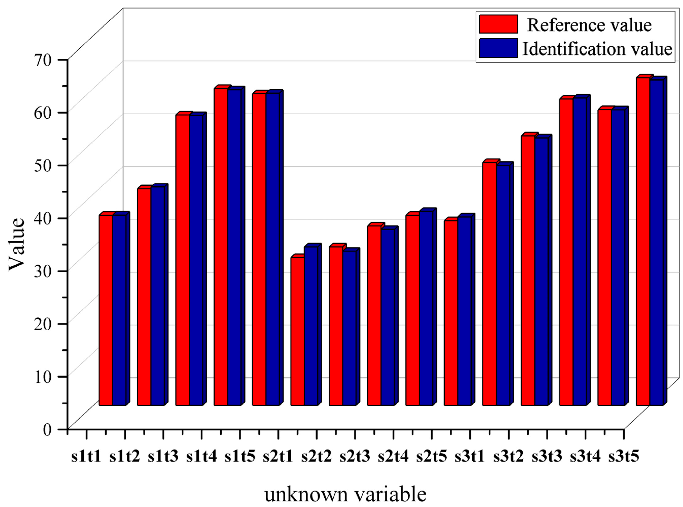
4.2. Inverse Characteristic Result

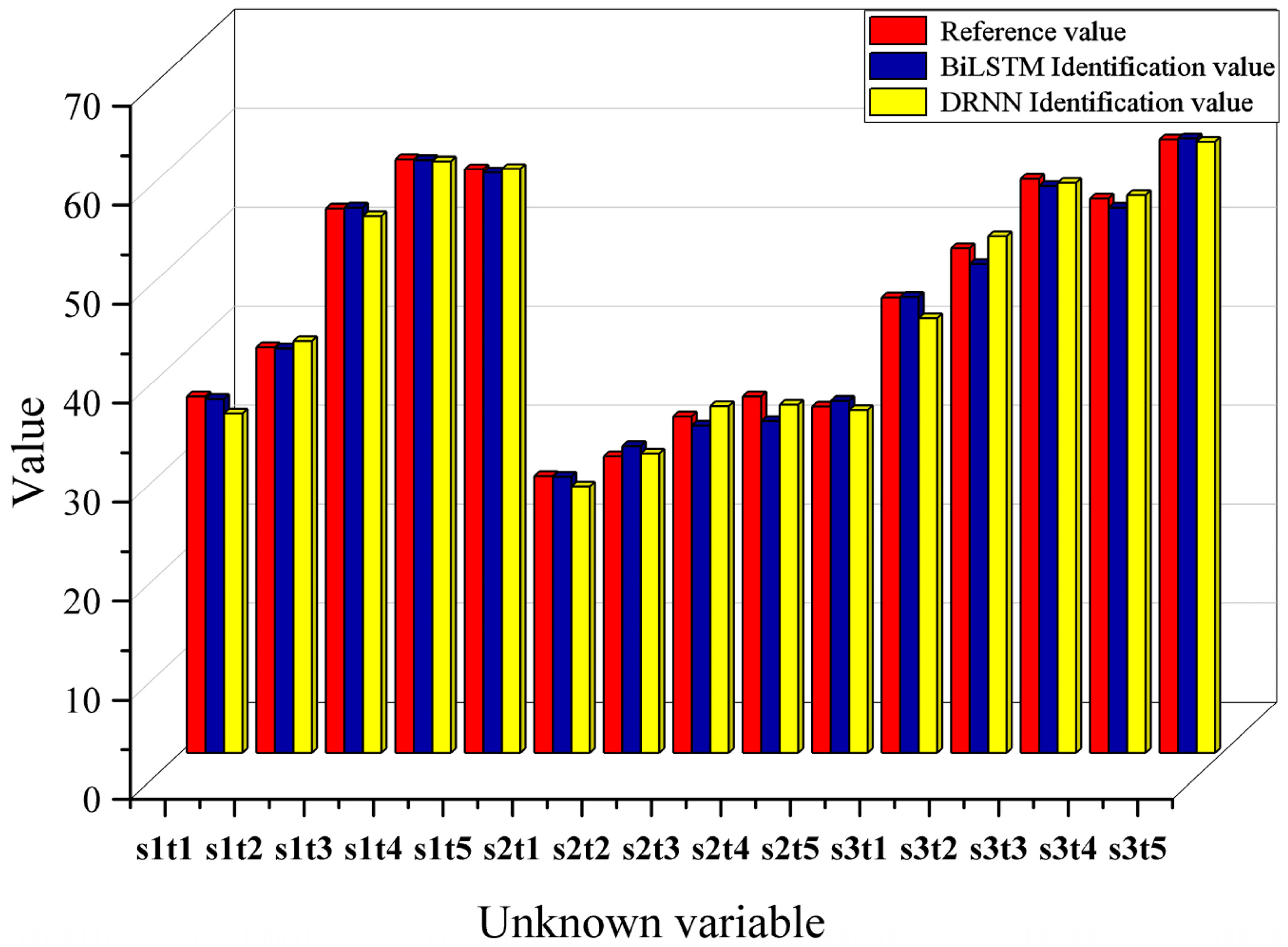
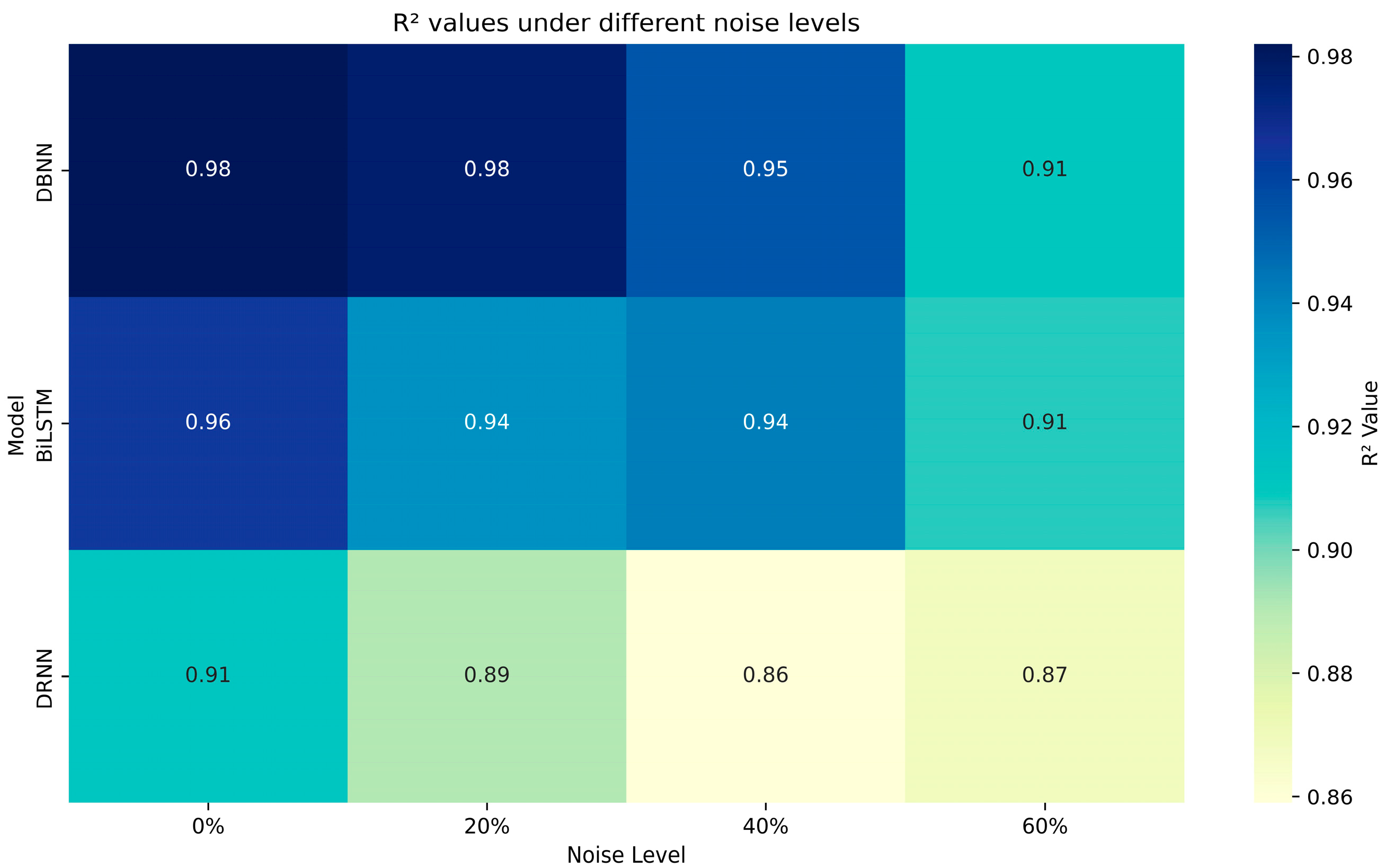
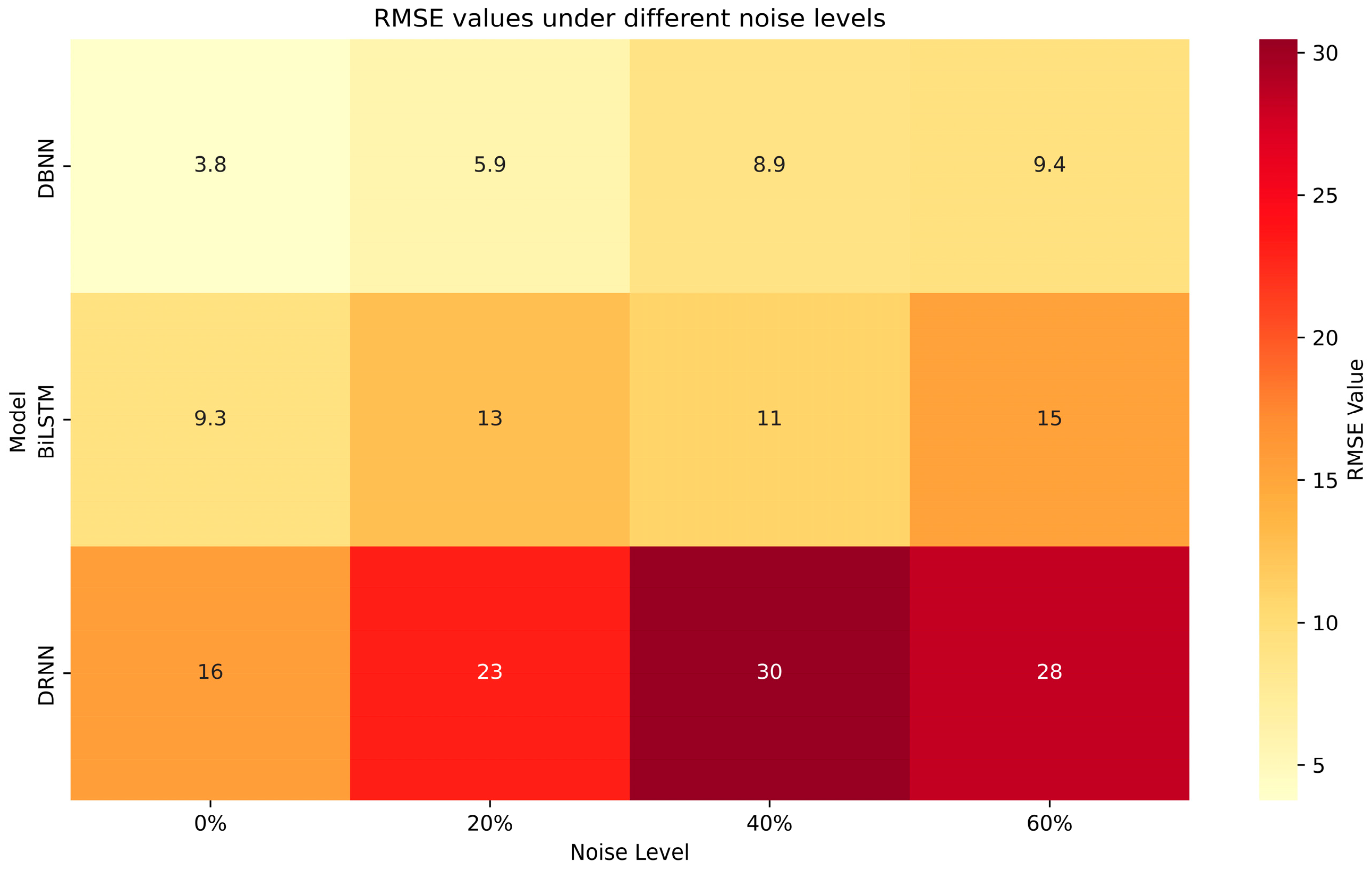
In this section, the focus of the study is on assessing the robustness of three surrogate models using the same parameters as in Experiment 4.1. However, unlike in Experiment 4.1, in this study, we initially set the three non-point sources as potential pollution sources. By identifying the release intensities of these three potential sources, we determine whether the site is an actual pollution source. If the simulation calculations identify that the release intensity of a potential source is zero, we can conclude that there is no pollution present at the site; if the identification results are approximate or identical to the actual reference values, it confirms that the site is indeed a pollution source. The specific variables to be identified are shown in

Table 3. Reference values of unknown variables to identify.

Unknown Variables to Identify	Reference Value
Fluxes of pollution source, S1T1 (g/d)	36
Fluxes of pollution source, S1T2 (g/d)	41
Fluxes of pollution source, S1T3 (g/d)	55
Fluxes of pollution source, S1T4 (g/d)	60
Fluxes of pollution source, S1T5 (g/d)	59
Fluxes of pollution source, S2T1 (g/d)	28
Fluxes of pollution source, S2T2 (g/d)	30
Fluxes of pollution source, S2T3 (g/d)	34
Fluxes of pollution source, S2T4 (g/d)	36
Fluxes of pollution source, S2T5 (g/d)	35
Fluxes of pollution source, S3T1 (g/d)	46
Fluxes of pollution source, S3T2 (g/d)	51
Fluxes of pollution source, S3T3 (g/d)	58
Fluxes of pollution source, S3T4 (g/d)	56
Fluxes of pollution source, S3T5 (g/d)	62

.

Furthermore, this study thoroughly considers the uncertainty introduced by noise in observational data, comparing the inversion accuracy of three deep learning methods. It selects the method with the highest accuracy for uncertainty analysis to assess the impact of noise on the inversion results. In this case, we deliberately introduce a quantified amount of noise into the surrogate models, making the robustness of the models a key indicator of their performance.

For this experiment, we initially undertook the identification and verification of potential pollution sources. Following the case introduction and the model parameters described in Section 4.1, we employ the highest accuracy surrogate model, the DBNN, for inversion simulation calculations. The identification results are displayed in

Table 4. The identification results obtained using the DBNN surrogate model for inversion are shown.

Unknown Variables	True Value	Inference Value Calculated by DBNN
S1T1	36	36.75
S1T2	41	41.99
S1T3	55	54.98
S1T4	60	60.12
S1T5	59	59.68
S2T1	28	28.76
S2T2	30	29.97
S2T3	34	34.36
S2T4	36	35.61
S2T5	35	35.89
S3T1	46	45.88
S3T2	51	51.74
S3T3	58	58.36
S3T4	56	56.50
S3T5	62	62.25

. According to these results, the values identified for S1, S2, and S3 are very close to the actual values. Based on the inversion outcomes, it is determined that S1, S2, and S3 are indeed genuine pollution sources, and this conclusion aligns with the actual situation.

During the study of the GCSI process, we observed that the monitoring well data contained noise. In previous studies, to test the robustness of inversion methods, a series of preset fixed noises were often added to the observation data. However, in this study, noise is randomly added to the observational data, represented as 0.5%, 1%, and 1.5%.

Table 5. Comparison of monitored values for DBNN under different noise conditions.

Unknown Variable	Reference Value	Estimation under Measurement Noise Level	0	0.005	0.010	0.015
S1T1	36		36.04	36.03	36.39	35.75
S1T2	41		41	40.95	40.86	40.88
S1T3	55		55	55.02	53.99	55.10
S1T4	60		60.01	60.08	59.69	59.92
S1T5	59		59	59.09	58.78	58.66
S2T1	28		28	27.82	28.08	27.93
S2T2	30		30	30.02	29.65	31.01
S2T3	34		34	34.09	33.90	33.07
S2T4	36		36.02	36.15	36.28	33.53
S2T5	35		34.99	34.99	36.82	35.56
S3T1	46		46.01	45.80	46.29	46.05
S3T2	51		51	51.17	50.88	49.44
S3T3	58		58.03	57.78	57.79	57.27
S3T4	56		55.96	55.95	56.33	55.09
S3T5	62		61.98	62.38	62.07	62.10

,

Table 6. Comparison of monitored values for BiLSTM under different noise conditions.

Unknown Variable	Reference Value	Estimation under Measurement Noise Level	0	0.005	0.010	0.015
S1T1	36		36	36.02	35.73	36.02
S1T2	41		41.01	41.07	41.16	41.34
S1T3	55		55	54.96	54.96	54.89
S1T4	60		60	60.18	60.30	59.75
S1T5	59		59	59.09	59.35	59.10
S2T1	28		27.98	28.05	28.29	30.00
S2T2	30		30	29.79	29.67	29.18
S2T3	34		34	33.99	34.25	33.35
S2T4	36		36	36.06	36.19	36.73
S2T5	35		35.02	35.11	34.61	35.69
S3T1	46		46.01	46.51	45.91	45.47
S3T2	51		50.96	51.03	53.11	50.61
S3T3	58		58	57.71	57.76	58.19
S3T4	56		56	56.12	56.39	55.97
S3T5	62		61.95	61.92	61.86	61.60

and

Table 7. Comparison of monitored values for DRNN under different noise conditions.

Unknown Variable	Reference Value	Estimation under Measurement Noise Level	0	0.005	0.010	0.015
S1T1	36		36	35.83	35.59	34.29
S1T2	41		41	41.02	40.75	41.62
S1T3	55		55.02	55.11	55.33	54.25
S1T4	60		59.99	59.75	60.09	59.79
S1T5	59		59	58.96	57.74	59.02
S2T1	28		28.02	28.36	27.63	26.94
S2T2	30		30	29.82	30.15	30.27
S2T3	34		34	34.05	32.94	35.04
S2T4	36		36	35.99	35.77	35.19
S2T5	35		34.96	34.87	34.88	34.64
S3T1	46		46	46.18	46.13	43.93
S3T2	51		51.08	50.93	50.66	52.22
S3T3	58		58	57.77	58.29	57.59
S3T4	56		55.95	56.14	55.96	56.35
S3T5	62		62	62.22	60.82	61.76

clearly show that under a noise level of 0%, the estimated values from S1T1 to S1T5, S2T1 to S2T5, and S3T1 to S3T5 for each period are closer to the actual true values. Therefore, we can infer that the pollution source began discharging contaminants into the aquifer starting from T1 and concluded at T5. This inference is consistent with the known history of pollution release.

It can be observed that for the same observation wells with noisy observational data, the values obtained by DBNN are closer to the actual measurement data compared to those obtained by BiLSTM and DRNN. Furthermore, DBNN also exhibits a lower average relative error in comparison to BiLSTM and DRNN, as shown in

Table 8. The mean errors of the three surrogate models after adding artificial noise.

	DBNN	BiLSTM	DRNN
average error value	0.24	0.28	0.32

, which presents the average errors of the three surrogate models.

Due to the addition of noise, the BiLSTM and DRNN methods experienced a decline in the accuracy of model training outcomes. However, the DBNN method was able to maintain the stability and accuracy of model training, even with varying degrees of noise present in the data. The primary source of this difference stems from the DBNN's unique architecture and training mechanism, which is reflected in the following aspects:

1. During groundwater pollution inversion simulations, BiLSTM and DRNN typically adopt an end-to-end training approach. Figure 14 shows the comparison between the monitored values and actual values in the BiLSTM and DRNN models after introducing 1.5% noise. This demonstrates that when identifying unknown pollution source variables, these two models need to learn the weights of all layers simultaneously. However, in this case, due to the complexity of the scenario and higher levels of noise, this learning strategy often leads to significant errors and is less effective than the layer-by-layer training approach of DBNN. Figure 15 also displays the comparison of DBNN monitored values with the actual values after introducing noise. Lacking a layer-by-layer pre-training mechanism, BiLSTM and DRNN are more sensitive to noise in the early stages of training and are prone to learning inaccurate features of the case under the misleading influence of noise.

2. In this case, when handling complex and variable datasets, robustness becomes a key consideration. DBNN employs layer-by-layer pre-training and an energy-based learning approach to deeply mine the intrinsic distribution of groundwater pollution data, thereby demonstrating high efficiency in managing noise within the data. This method grants DBNN significant robustness, enabling it to effectively accomplish the research tasks. In contrast, although BiLSTM and DRNN are capable of handling complex relationships within datasets, they are relatively fragile in terms of noise management.

By comparing the performance of DBNN, BiLSTM, and DRNN surrogate models in measuring unknown variables under conditions of artificial noise, the data clearly display the relative errors due to the impact of noise on the models. The results distinctly show that DBNN has a significant advantage in resisting noise influence. As the proportion of noise increases, the DBNN model’s ability to match monitoring identification values with actual values remains notably superior to the other two models, demonstrating stronger robustness.

Overall, DBNN is capable of effectively simulating dynamic groundwater pollution environments while maintaining a high level of robustness. By utilizing DBNN, we can significantly enhance the resilience of surrogate models against the inevitable noise interference in real-world groundwater pollution simulations, thereby ensuring the accuracy and reliability of data processing.

4.3. Ablation Study

This chapter aims to further compare the effectiveness of the three surrogate models used in the articles DBNN, BiLSTM, and DRNN for the GCSI task. First, due to the different internal structures of the three surrogate models, ablation studies are designed for each separately. To ensure the fairness of the ablation studies, a proportional reduction method for the ablation level is employed. For the DBNN and DRNN models, the variable for ablation is the reduction of the original number of layers proportionally, while for the BiLSTM, the number of LSTM units per layer is reduced. Based on the original number, the reductions are 20%, 40%, and 60%, respectively, without changing other training parameters such as batch size and learning rate. In the results, simplified functional layers are used to replace the removed layers when reductions are made, ensuring that these surrogate layers are as functionally similar as possible by observing the impact of different proportions in the ablation studies on the surrogate models, as shown in Figure 16 and Figure 17.

This heatmap illustrates the R² metric values of the three models (DBNN, BiLSTM, DRNN) under different proportional ablation levels (20%, 40%, and 60%). The R² value represents the model’s goodness of fit, indicating how much of the variance in the data is explained by the model. The color gradient in the heatmap ranges from deep blue to light yellow, representing high to low R² values. Across all ablation levels, the DBNN model demonstrates the most stable and outstanding performance, with R² values decreasing from 0.982 to 0.910, showing strong robustness against ablation. The BiLSTM model performs well under 20% and 40% ablation, with R² values of 0.936 and 0.942, respectively, but drops to 0.908 under 60% ablation. Although still performing well, it is slightly inferior to DBNN. The DRNN model is the most sensitive to ablation, with R² values dropping from 0.911 to 0.859 and slightly recovering to 0.869 under 60% ablation, but overall, it does not perform as well as DBNN and BiLSTM. In summary, the DBNN model exhibits the highest goodness of fit under various ablation levels, followed by BiLSTM, while DRNN performs relatively poorly at all ablation levels.

Figure 17 shows the RMSE values of the three models under different proportional ablation levels, used to evaluate model performance across varying degrees of ablation. The color gradient ranges from light yellow to deep red, representing low to high RMSE values. The DBNN model exhibits outstanding performance at all ablation levels, with RMSE values increasing from 3.8 to 9.4, demonstrating strong robustness and stability against data ablation. The BiLSTM model shows relatively low RMSE values under 0% and 40% ablation, at 9.3 and 11, respectively, but the RMSE values increase to 13 and 15 under 20% and 60% ablation, indicating some fluctuations. The DRNN model is the most sensitive to ablation, with an RMSE value of 16 under 0% ablation, significantly rising to 23 and 30 under 20% and 40% ablation, and slightly decreasing to 28 under 60% ablation, but still the highest overall.

In summary, the DBNN model performs best under varying ablation levels, with the lowest RMSE, followed by BiLSTM, while DRNN has the highest RMSE across all ablation levels. This indicates that DBNN is more robust and stable in handling incomplete or missing data, whereas DRNN is more vulnerable. The results of the ablation study suggest that the DBNN model is more suitable for applications in imperfect data conditions.

In this ablation study for GCSI tasks, we systematically evaluated the performance of three models: DBNN, BiLSTM, and DRNN. The experimental results show that DBNN exhibits significant robustness and stability across different ablation levels, with minimal fluctuations in R² and RMSE values, demonstrating its high adaptability to structural simplification. This superiority can be attributed to DBNN layer-by-layer pre-training and unsupervised learning mechanism, which allows each layer to independently capture and represent features. Specifically, DBNN excels in handling the complex and high-dimensional data of GCSI tasks by stacking RBM layer by layer to extract high-level features. The unsupervised pre-training of RBM provides a solid feature foundation, alleviating the burden on subsequent supervised learning enabling DBNN to maintain high performance even under ablation conditions.

In contrast, the performance of BiLSTM and DRNN in the ablation studies was relatively unstable. BiLSTM relies on bidirectional LSTM units to capture both forward and backward dependencies in sequential data. When the number of LSTM units is reduced, this capability to capture temporal dependencies significantly diminishes, resulting in increased performance fluctuations. The disadvantage of the bidirectional structure during ablation is that the model needs to retain the same amount of information within the reduced units, making it highly sensitive to structural changes and causing greater volatility. While BiLSTM’s advantage lies in its ability to simultaneously capture bidirectional information in sequence data, which is effective for complex time-series tasks, its performance is significantly impacted after structural simplification, with a marked increase in sensitivity and instability.

The disadvantages of DRNN in the ablation studies are primarily reflected in its reliance on the multi-layer recurrent structure to capture long-term dependencies. When the number of layers is reduced, the model loses some of the time-step information provided by the recurrent layers, leading to a significant decline in its ability to model long-term sequential data. Since the recurrent units in DRNN depend on the output of preceding layers, a reduction in the number of layers directly impacts the overall memory capacity and the efficiency of sequential information transmission in the model. Although the DRNN multi-layer structure is capable of capturing complex temporal dependencies, its memory and prediction capabilities significantly diminish after structural simplification, revealing its high dependency on and vulnerability to long-term dependencies.

In the task of GCSI, the precise identification and localization of groundwater pollution sources are crucial. Groundwater pollution data typically exhibit high dimensionality, non-linearity, and complexity. The layer-wise pre-training and unsupervised learning strategy of DBNN demonstrates unique advantages in handling these complex data, allowing for more accurate capture of the spatial distribution and temporal trends of pollution sources. In contrast, BiLSTM and DRNN show significant performance degradation in addressing such complex tasks due to their high dependence on structural integrity.

In summary, the ablation studies, by gradually reducing the number of model layers or units, reveal the contribution of each structural component to the overall model performance. The layer-wise pre-training and unsupervised learning strategy of DBNN enables it to maintain high robustness and stability during structural simplification, whereas BiLSTM and DRNN, due to their high reliance on internal structural integrity, exhibit significant performance degradation in the ablation studies. By comparing the strengths and weaknesses of DBNN, BiLSTM, and DRNN, we conclude that DBNN, owing to its unique training method and structural design, significantly outperforms BiLSTM and DRNN in GCSI tasks, making it the more suitable model choice. This provides critical theoretical support and experimental evidence for future model optimization and application.

5. Conclusions

This study conducted an in-depth exploration of the problem of GCSI, focusing on the spatiotemporal characteristics of contamination sources and hydraulic conductivity. By designing case studies similar to actual non-point source pollution events, we performed a comprehensive comparative evaluation of the three proposed deep learning surrogate models (DBNN, BiLSTM, and DRNN). The results validated the effectiveness of these models in GCSI tasks and revealed their performance in handling complex, high-dimensional data.

1. Our research shows that DBNN demonstrates significant model adaptability and excellent computational accuracy when dealing with high-dimensional nonlinear inverse problems. Among all the models, DBNN exhibited stronger stability and higher predictive accuracy. This performance advantage makes DBNN not only outstanding in the current study but also widely applicable in other hydrogeological fields that require processing complex environmental data. However, there is still room for improvement in DBNN extrapolation capabilities. Future research should focus on further optimizing DBNN model structure and solute transport simulation to enhance its performance in more complex scenarios.

2. The experimental results under different noise levels indicate that although noise can impact prediction accuracy, DBNN still maintains high predictive accuracy, demonstrating its strong resistance to interference. This finding is crucial for practical applications, as noise interference is inevitable in actual environmental monitoring data. Ensuring the robustness of the model under noisy conditions is one of the important directions for future research. In subsequent studies, we will further explore and develop more noise-resistant techniques to enhance the model’s reliability in noisy environments.

3. Accurate selection of surrogate model parameters is critical for the success of GCSI tasks. This study focused on analyzing model performance in non-point source pollution scenarios. Future research should expand to include point source and linear pollution scenarios to fully validate the generality and practicality of the proposed methods. Through these extended studies, we will gain a more comprehensive understanding and optimization of the application of deep learning models in different types of contamination source identification.

In summary, our research further confirms the unique advantages of DBNN in handling complex, high-dimensional nonlinear problems and demonstrates the potential of deep learning technology in groundwater contamination source identification. Future research will continue to optimize the structure of these models, expand their applicability in different geological environments, and further enhance their practical value in groundwater contamination management. We believe that as these models are continuously improved and the technology optimized, deep learning will play an increasingly important role in global water resource protection and environmental management.

References

1. Lapworth, D.J.; Boving, T.B.; Kreamer, D.K.; Kebede, S.; Smedley, P.L. Groundwater quality: Global threats, opportunities and realising the potential of groundwater. Sci. Total. Environ. 2022, 811, 152471. [Google Scholar] [CrossRef]
2. Ayvaz, M.T. A linked simulation–optimization model for solving the unknown groundwater pollution source identification problems. J. Contam. Hydrol. 2010, 117, 46–59. [Google Scholar] [CrossRef] [PubMed]
3. Mahar, P.S.; Datta, B. Optimal identification of ground-water pollution sources and parameter estimation. J. Water Res. Plan. Man. 2001, 127, 20–29. [Google Scholar] [CrossRef]
4. Liu, X.; Zhai, Z.J. Prompt tracking of indoor airborne contaminant source location with probability-based inverse multi-zone modeling. Build. Environ. 2009, 44, 1135–1143. [Google Scholar] [CrossRef]
5. van der Velde, Y.; de Rooij, G.H.; Rozemeijer, J.C.; van Geer, F.C.; Broers, H.P. Nitrate response of a lowland catchment; on the relation between stream concentration and travel time distribution dynamics. Water Resour. Res. 2010, 46, W11534. [Google Scholar] [CrossRef]
6. Zhao, Y.; Qu, R.; Xing, Z.; Lu, W. Identifying groundwater contaminant sources based on a KELM surrogate model together with four heuristic optimization algorithms. Adv. Water Resour. 2020, 138, 103540. [Google Scholar] [CrossRef]
7. Li, J.; Lu, W.; Wang, H.; Fan, Y.; Chang, Z. Groundwater contamination source identification based on a hybrid particle swarm optimization-extreme learning machine. J. Hydrol 2020, 584, 124657. [Google Scholar] [CrossRef]
8. Guo, Q.; Dai, F.; Zhao, Z. Comparison of Two Bayesian-MCMC Inversion Methods for Laboratory Infiltration and Field Irrigation Experiments. Int. J. Environ. Res. Public Health 2020, 17, 1108. [Google Scholar] [CrossRef]
9. Zhang, J.; Vrugt, J.A.; Shi, X.; Lin, G.; Wu, L.; Zeng, L. Improving Simulation Efficiency of MCMC for Inverse Modeling of Hydrologic Systems With a Kalman-Inspired Proposal Distribution. Water Resour. Res. 2020, 56, e2019WR025474. [Google Scholar] [CrossRef]
10. Datta, B.; Chakrabarty, D.; Dhar, A. Identification of unknown groundwater pollution sources using classical optimization with linked simulation. J. Hydro-Environ. Res. 2011, 5, 25–36. [Google Scholar] [CrossRef]
11. Seyedpour, S.M.; Kirmizakis, P.; Brennan, P.; Doherty, R.; Ricken, T. Optimal remediation design and simulation of groundwater flow coupled to contaminant transport using genetic algorithm and radial point collocation method (RPCM). Sci. Total. Environ. 2019, 669, 389–399. [Google Scholar] [CrossRef]
12. Gaur, S.; Chahar, B.R.; Graillot, D. Analytic elements method and particle swarm optimization based simulation–optimization model for groundwater management. J. Hydrol. 2011, 402, 217–227. [Google Scholar] [CrossRef]
13. Wang, Z.; Lu, W. Groundwater Contamination Source Recognition Based on a Two-Stage Inversion Framework with a Deep Learning Surrogate. Water 2024, 16, 1907. [Google Scholar] [CrossRef]
14. Hussain, M.S.; Javadi, A.A.; Ahangar-Asr, A.; Farmani, R. A surrogate model for simulation–optimization of aquifer systems subjected to seawater intrusion. J. Hydrol. 2015, 523, 542–554. [Google Scholar] [CrossRef]
15. Neupauer, R.M.; Borchers, B.; Wilson, J.L. Comparison of inverse methods for reconstructing the release history of a groundwater contamination source. Water Resour. Res. 2000, 36, 2469–2475. [Google Scholar] [CrossRef]
16. Asher, M.J.; Croke, B.F.W.; Jakeman, A.J.; Peeters, L.J.M. A review of surrogate models and their application to groundwater modeling. Water Resour. Res. 2015, 51, 5957–5973. [Google Scholar] [CrossRef]
17. Secci, D.; Molino, L.; Zanini, A. Contaminant source identification in groundwater by means of artificial neural network. J. Hydrol. 2022, 611, 128003. [Google Scholar] [CrossRef]
18. Knoll, L.; Breuer, L.; Bach, M. Large scale prediction of groundwater nitrate concentrations from spatial data using machine learning. Sci. Total. Environ. 2019, 668, 1317–1327. [Google Scholar] [CrossRef]
19. Daliakopoulos, I.N.; Coulibaly, P.; Tsanis, I.K. Groundwater level forecasting using artificial neural networks. J. Hydrol. 2005, 309, 229–240. [Google Scholar] [CrossRef]
20. Baudron, P.; Alonso-Sarría, F.; García-Aróstegui, J.L.; Cánovas-García, F.; Martínez-Vicente, D.; Moreno-Brotóns, J. Identifying the origin of groundwater samples in a multi-layer aquifer system with Random Forest classification. J. Hydrol. 2013, 499, 303–315. [Google Scholar] [CrossRef]
21. Rashid, M.; Bari, B.S.; Yusup, Y.; Kamaruddin, M.A.; Khan, N. A Comprehensive Review of Crop Yield Prediction Using Machine Learning Approaches With Special Emphasis on Palm Oil Yield Prediction. IEEE Access. 2021, 9, 63406–63439. [Google Scholar] [CrossRef]
22. Barzegar, R.; Moghaddam, A.A.; Deo, R.; Fijani, E.; Tziritis, E. Mapping groundwater contamination risk of multiple aquifers using multi-model ensemble of machine learning algorithms. Sci. Total. Environ. 2018, 621, 697–712. [Google Scholar] [CrossRef] [PubMed]
23. Siade, A.J.; Cui, T.; Karelse, R.N.; Hampton, C. Reduced-Dimensional Gaussian Process Machine Learning for Groundwater Allocation Planning Using Swarm Theory. Water Resour. Res. 2020, 56, e2019WR026061. [Google Scholar] [CrossRef]
24. Rodriguez-Galiano, V.; Mendes, M.P.; Garcia-Soldado, M.J.; Chica-Olmo, M.; Ribeiro, L. Predictive modeling of groundwater nitrate pollution using Random Forest and multisource variables related to intrinsic and specific vulnerability: A case study in an agricultural setting (Southern Spain). Sci. Total. Environ. 2014, 476–477, 189–206. [Google Scholar] [CrossRef] [PubMed]
25. Singh, R.M.; Datta, B. Artificial neural network modeling for identification of unknown pollution sources in groundwater with partially missing concentration observation data. Water Resour. Manag. 2007, 21, 557–572. [Google Scholar] [CrossRef]
26. Motevalli, A.; Naghibi, S.A.; Hashemi, H.; Berndtsson, R.; Pradhan, B.; Gholami, V. Inverse method using boosted regression tree and k-nearest neighbor to quantify effects of point and non-point source nitrate pollution in groundwater. J. Clean. Prod. 2019, 228, 1248–1263. [Google Scholar] [CrossRef]
27. Kouadri, S.; Elbeltagi, A.; Islam, A.R.M.T.; Kateb, S. Performance of machine learning methods in predicting water quality index based on irregular data set: Application on Illizi region (Algerian southeast). Appl. Water Sci. 2021, 11, 190. [Google Scholar] [CrossRef]
28. Sze, V.; Chen, Y.; Yang, T.; Emer, J.S. Efficient Processing of Deep Neural Networks: A Tutorial and Survey. Proc. IEEE 2017, 105, 2295–2329. [Google Scholar] [CrossRef]
29. Liang, T.; Glossner, J.; Wang, L.; Shi, S.; Zhang, X. Pruning and quantization for deep neural network acceleration: A survey. Neurocomputing 2021, 461, 370–403. [Google Scholar] [CrossRef]
30. Jiang, Z.; Tahmasebi, P.; Mao, Z. Deep residual U-net convolution neural networks with autoregressive strategy for fluid flow predictions in large-scale geosystems. Adv. Water Resour. 2021, 150, 103878. [Google Scholar] [CrossRef]
31. Yan, L.; Feng, J.; Hang, T.; Zhu, Y. Flow interval prediction based on deep residual network and lower and upper boundary estimation method. Appl. Soft Comput. 2021, 104, 107228. [Google Scholar] [CrossRef]
32. Murad, A.; Pyun, J. Deep Recurrent Neural Networks for Human Activity Recognition. Sensors 2017, 17, 2556. [Google Scholar] [CrossRef]
33. Chen, Z.; Ma, M.; Li, T.; Wang, H.; Li, C. Long sequence time-series forecasting with deep learning: A survey. Inf. Fusion 2023, 97, 101819. [Google Scholar] [CrossRef]
34. Vu, M.; Jardani, A.; Massei, N.; Fournier, M. Reconstruction of missing groundwater level data by using long short-term memory (LSTM) deep neural network. J. Hydrol. 2021, 597, 125776. [Google Scholar] [CrossRef]
35. Vu, M.T.; Jardani, A.; Massei, N.; Deloffre, J.; Fournier, M.; Laignel, B. Long-run forecasting surface and groundwater dynamics from intermittent observation data: An evaluation for 50 years. Sci. Total Environ. 2023, 880, 163338. [Google Scholar] [CrossRef] [PubMed]
36. Xu, R.; Hu, S.; Wan, H.; Xie, Y.; Cai, Y.; Wen, J. A unified deep learning framework for water quality prediction based on time-frequency feature extraction and data feature enhancement. J. Environ. Manag. 2024, 351, 119894. [Google Scholar] [CrossRef] [PubMed]
37. Sohn, I. Deep belief network based intrusion detection techniques: A survey. Expert Syst. Appl. 2021, 167, 114170. [Google Scholar] [CrossRef]
38. Pan, Z.; Lu, W.; Chang, Z.; Wang, H. Simultaneous identification of groundwater pollution source spatial-temporal characteristics and hydraulic parameters based on deep regularization neural network-hybrid heuristic algorithm. J. Hydrol. 2021, 600, 126586. [Google Scholar] [CrossRef]
39. Anul Haq, M.; Khadar Jilani, A.; Prabu, P. Deep Learning Based Modeling of Groundwater Storage Change. Comput. Mater. Contin. 2022, 70, 4599–4617. [Google Scholar] [CrossRef]
40. Jiang, S.; Fan, J.; Xia, X.; Li, X.; Zhang, R. An Effective Kalman Filter-Based Method for Groundwater Pollution Source Identification and Plume Morphology Characterization. Water 2018, 10, 1063. [Google Scholar] [CrossRef]
41. Yuan, X.; Ou, C.; Wang, Y.; Yang, C.; Gui, W. A novel semi-supervised pre-training strategy for deep networks and its application for quality variable prediction in industrial processes. Chem. Eng. Sci. 2020, 217, 115509. [Google Scholar] [CrossRef]
42. Li, J.; Wu, Z.; He, H.; Lu, W. Identifying groundwater contamination sources based on the hybrid grey wolf gradient algorithm and deep belief neural network. Stoch. Environ. Res. Risk A 2023, 37, 1697–1715. [Google Scholar] [CrossRef]
43. Karhunen, J.; Raiko, T.; Cho, K. Unsupervised deep learning: A short review. Adv. Indep. Compon. Anal. Learn. Mach. 2015, 125–142. [Google Scholar] [CrossRef]
44. Hinton, G.E.; Osindero, S.; Teh, Y. A Fast Learning Algorithm for Deep Belief Nets. Neural Comput. 2006, 18, 1527–1554. [Google Scholar] [CrossRef]
45. Wang, Y.; Zou, R.; Liu, F.; Zhang, L.; Liu, Q. A review of wind speed and wind power forecasting with deep neural networks. Appl. Energ. 2021, 304, 117766. [Google Scholar] [CrossRef]
46. He, K.; Zhang, X.; Ren, S.; Sun, J. Deep Residual Learning for Image Recognition. In Proceedings of the IEEE Conference On Computer Vision and Pattern Recognition (CVPR), Las Vegas, NV, USA, 27–30 June 2016. [Google Scholar]
Figure 1. Technical Roadmap for GCSI.
Water 16 02449 g001
Figure 2. The schematic of RBM. In the diagram, the red neurons at the top form the hidden layer, while the blue neurons constitute the visible layer.
Water 16 02449 g002
Figure 3. The schematic of DBNN.
Water 16 02449 g003
Figure 4. Schematic diagram of the internal structure of LSTM.
Water 16 02449 g004
Figure 5. Schematic diagram of the internal structure of BiLSTM.
Water 16 02449 g005
Figure 6. The schematic of ResBlock.
Water 16 02449 g006
Figure 7. Case overview of the contaminated source.
Water 16 02449 g007
Figure 8. Contaminant concentration distribution during the stress periods: (a) period T1, (b) period T2, (c) period T3 and (d) period T5.
Water 16 02449 g008
Figure 9. The case study uses a multivariate joint distribution plot of variables obtained through Latin Hypercube Sampling.
Water 16 02449 g009
Figure 10. Comparison chart of evaluation metrics for the three surrogate models: DBNN, BiLSTM, and DRNN.
Water 16 02449 g010
Figure 11. (a) The fitting accuracy of the DBNN surrogate model. (b) Illustration of the training process of the DBNN.
Water 16 02449 g011
Figure 12. (a) The fitting accuracy of the BiLSTM surrogate model. (b) Illustration of the training process of the BiLSTM.
Water 16 02449 g012
Figure 13. (a) The fitting accuracy of the DRNN surrogate model. (b) Illustration of the training process of the DRNN.
Water 16 02449 g013
Figure 14. Comparison of the monitored values and true values after introducing 1.5% artificial noise in the BiLSTM and DRNN surrogate models.
Water 16 02449 g014
Figure 15. Comparison of the monitored values and true values after introducing 1.5% artificial noise in the DBNN surrogate model.
Water 16 02449 g015
Figure 16. The impact of different proportions in ablation studies on the R2 values of the three surrogate models.
Water 16 02449 g016
Figure 17. The impact of different proportions in ablation studies on the RMSE values of the three surrogate models.
Water 16 02449 g017