Abstract
The interaction of water flow, ice, and structures is common in fluvial ice processes, particularly around Ice Control Structures (ICSs) that are used to manage and prevent ice jam floods. To evaluate the effectiveness of ICSs, it is essential to understand the complex interaction between water flow, ice and the structure. Numerical modeling is a valuable tool that can facilitate such understanding. Until now, classical Eulerian mesh-based methods have not been evaluated for the simulation of ice interaction with ICS. In this paper we evaluate the capability, accuracy, and efficiency of a coupled Computational Fluid Dynamic (CFD) and multi-body motion numerical model, based on the mesh-based FLOW-3D V.2023 R1 software for simulation of ice-structure interactions in several benchmark cases. The model’s performance was compared with results from meshless-based models (performed by others) for the same laboratory test cases that were used as a reference for the comparison. To this end, simulation results from a range of dam break laboratory experiments were analyzed, encompassing varying numbers of floating objects with distinct characteristics, both in the presence and absence of ICS, and under different downstream water levels. The results show that the overall accuracy of the FLOW-3D model under various experimental conditions resulted in a RMSE of 0.0534 as opposed to an overall RMSE of 0.0599 for the meshless methods. Instabilities were observed in the FLOW-3D model for more complex phenomena that involve open boundaries and a larger number of blocks. Although the FLOW-3D model exhibited a similar computational time to the GPU-accelerated meshless-based models, constraints on the processors speed and the number of cores available for use by the processors could limit the computational time.
1. Introduction
The interaction of ice with hydraulic structures, such as dams and bridges, is common in cold-region rivers and can pose substantial risks to infrastructure, environment, and human safety. It is also a common feature of Ice Control Structures (ICSs) that are designed to manage the movement of ice within rivers and streams. They include ice booms, ice retention weirs, and ice deflectors and are key measures for mitigating ice jams and resulting floods and infrastructural damage [1,2,3,4]. Effective ice jam management through ICS mitigates the impacts on ecology and socio-economics and protects infrastructure from ice-related damage [5,6,7].
Due to climate change and the increased likelihood of mid-winter breakups, it is crucial to periodically reevaluate ICSs for their effectiveness in controlling ice jam floods [8,9]. Various methods are used to assess ICS performance, including historical and field observations, laboratory experiments, and numerical simulations. Historical studies provide insights into ice jam floods before and after ICS construction [10]. Laboratory experiments are useful for new structure implementations or when numerical approaches fall short [11,12]. Numerical modeling is increasingly important for evaluating ICS under various conditions, from initial implementation [13] to modification and removal impacts [14,15]. By leveraging numerical modeling, researchers can thoroughly evaluate ICS capabilities in managing ice jam floods and preventing related damage. The interaction between fast flowing water, ice, and ICSs is complex and requires sophisticated modeling and analysis to predict and manage effectively. These advanced numerical models should initially be validated through simple test cases, such as evaluating the effects of variations in triangular slope, before being applied to more complex scenarios [16,17].
Numerical models for simulating river ice dynamics range from simple one-dimensional (1D) models like HEC-RAS [18], CRISP1D [19], and RIVICE [20] to sophisticated two-dimensional (2D) models such as DynaRICE [21]. Shen [22] reviewed 2D models for ice processes, including jamming and release. The Discrete Element Method (DEM) [23], reviewed by Tuhkuri and Polojärvi [24], is primarily used for sea ice but has also been applied to river ice and ICS studies [25,26]. These models often couple DEM with analytical or depth-averaged hydrodynamics, practical for large-scale applications but insufficient for complex three-dimensional interactions in ICS problems. Advances in continuum-based mesh-free Lagrangian methods like Smoothed Particle Hydrodynamics (SPH) [27] and Moving Particle Semi-Implicit (MPS) [28] provide flexibility for simulating dynamic fluid flows. When combined with DEM, these methods effectively model dynamic fluid flow and multi-body solid interactions [29,30], suitable for river ice simulations. Recent applications of these techniques in river ice problems are shown by Amaro et al. [31] and Billy et al. [32,33]. Furthermore, classical Eulerian methods like those using, fixed, moving and deforming meshes [34] have not been evaluated for the simulation of ice interaction with ICS. FLOW-3D, a commercial mesh-based Eulerian model, is an example of such models which uses the Volume of Fluid (VOF) method for fluid flow simulation [35,36,37,38] and have different application from river to coastal engineering [39] and incorporates a General Moving Objects (GMO) model based on DEM and the Fractional Area Volume Obstacle Representation (FAVOR) technique. While application of GMO model was evaluated by Wei [40] and Wang et al. [41], its application in ice engineering needs further study [42].
In this study, the FLOW-3D numerical model is evaluated to determine its capabilities to simulate ice blocks movement and their interaction with ICSs. Additionally, the accuracy and efficiency of the numerical model is assessed. To this end, the model is applied to a series of dam break scenarios previously tested by Amaro et al. [31] and Billy et al. [33]. The case studies cover several levels of complexities including the variation of the number of moving blocks, adjusting the water level downstream of the tank, and incorporating an ICS within the tank. Subsequently, simulations were conducted for a straight channel with different flow conditions featuring an ICS and additional blocks to mimic natural conditions. In all cases, the results of the FLOW-3D numerical model (referred to as the “current numerical model”) were compared both qualitatively and quantitatively to laboratory experiments and other numerical models. These steps demonstrate the model’s capabilities in handling wave-ice interactions and ice jam simulations, as well as the accuracy of the results. In the final phase, the computational time is evaluated to assess the efficiency of the numerical simulations.
2. Methodology
The methodology is divided into four sections. The first section describes the test cases selected for the basis of comparison and validation of the results of the numerical modeling, along with the rationale for their selection. The second section details the numerical modeling methods used in the current study and provides a concise explanation of the formulas and approaches implemented in the current numerical model. Following by the third section which describes the model setup and the parameters values chosen for this study. Finally, the fourth section describes the evaluation criteria used to assess the accuracy of the current numerical model.
2.1. Test Cases
In this section, an overview of the test cases (TC), used for the evaluation of the current numerical model is presented. The TC involved various dam-break cases with floating ice blocks, with and without downstream structures, based on the experimental and numerical works of Amaro et al. [31] and Billy et al. [33]. They were selected for their simplicity, abundance of quality experimental and numerical data, and inclusion of characteristics that mimic ice-structure interactions in real fluvial systems.
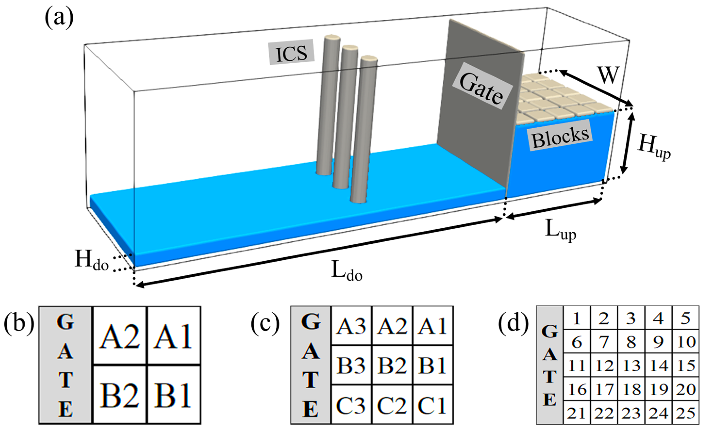
Figure 1 presents schematic of the TC and Table 1 summarize their characteristics. The experimental dimensions utilized by Amaro et al. [31] and Billy et al. [33] is similar to those employed in previous experimental studies [43,44,45]. It is important to note that these experiments were not directly designed to replicate field observations from a specific study site, but rather to assess the capabilities of numerical models to simulate such dynamic events. The detail of the experimental procedures, experimental setup scaling, material properties definition and estimation, and the numerical methods used for their simulations can be found in Amaro et al. [31] and Billy et al. [33].

Figure 1.
(a) Schematic view of the TC, and arrangement of blocks with (b) TC4, (c) TC9, and (d) TC25. Hdo and Hup show downstream and upstream water depth, Ldo and Lup indicate water length downstream and upstream of the gate, and W displays the width of the tank. Note that TC4 and TC9 did not have ICS downstream of the gate.

Table 1.
Details of experimental setup and materials used in the test cases as well as the numerical parameters used for respective simulations.
The first and second TC, TC4 and TC9, were proposed by Amaro et al. [31] and involve dam-breaks, with different downstream depths, with 4 and 9 floating artificial ice blocks (for TC4 and TC9, respectively), without any downstream structure. Experiments were conducted at the hydraulic laboratory of Polytechnique Montreal. Amaro et al. [31] used a fully Lagrangian particle-based numerical method, based on DEM and MPS methods (within their in-house model MPARS) to simulate their TCs. In total, eight different scenarios were simulated as shown in Table 1. In absence of structures, these test cases evaluate the ability of the present model in simulation of wave-ice interaction simulation.
The third TC, TC25, is based on the experimental and numerical study of Billy et al. [33] in the same facility as the previous TC. It involves dam-break, with 25 floating ice blocks with several piers downstream of the dam replicates as an ICS.
Billy et al. [33] maintained fixed water depth for both upstream and downstream and performed two experimental scenarios utilizing two different materials for the blocks, real and artificial PP (Polypropylene) ice blocks (Table 1). Billy et al. [33] simulated these TC using the DualSPHysics open-source model, which is based on SPH and DEM particle-based numerical methods.
Several factors influenced the selection of these TC for the objectives of this research. Firstly, detailed and comprehensive experimental data as well as referenced numerical modeling results are available for these TC. Secondly, the TC incrementally add complexity, which is crucial for studying wave-ice-structure interactions near ICS. In TC4 a dam break scenario with 4 blocks is presented, and then the number of blocks increased to 9 blocks for TC9, both with varying downstream water depths, which introduces greater complexity to the analysis. TC25 further increase the complexity by not only increasing the number of blocks to 25 but also incorporating ICS, thereby enriching the study’s ability to simulate more intricate interactions. Additionally, TC25 compares the use of real ice versus artificial ice for simulating water and ice movement alongside ICS. One should mention that in the reference experimental result, up to three repetitions (here referred as R1, R2, and R3) were performed to confirm the repeatability of the results. Limitations on the laboratory TC and reasons for missing data of laboratory TC are explained in Amaro et al. [31] and Billy et al. [33].
2.2. Numerical Methods
For this research, the commercial modeling software FLOW-3D V.2023 R1 was employed. Detailed governing equations and the numerical methods are extensively documented in the software’s manual [46]. An overview of the procedures employed is provided here. In this study, the system is modeled in two phases: the fluid phase, which is simulated using the CFD module, and the solid phase, involving rigid blocks, which is solved using the DEM-like rigid body’s motion module. The modeling framework independently solves separate sets of governing equations for each phase and integrates their interactions through a coupling algorithm.
For the problems that involve moving objects interacted with a free surface fluid flow, the flow governing equations include the continuity (Equation (1)) and momentum (Equation (2)) equations, as well as a transport equation for the Volume of Fluid (VOF) (Equation (3)) used to tracking the free surface.
where, is the fluid density, is time, is the fluid velocity, is the volume fraction, the area fraction, the pressure, the viscous stress tensor, gravity, and the fluid fraction.
The rigid body’s motion is decomposed into translational (Equation (4)) and rotational (Equation (5)) components given by [46,47,48]:
where, represents the total force, denotes the mass of the rigid body, represents translational velocity, is the total torque about the center of mass G, is the moment of inertia tensor about G within a body-fitted reference system, and represents angular velocity. The velocity of any point on a rigid body can be expressed as the sum of the velocity of a selected base point on the object plus the velocity resulting from the object’s rotation about that base point. In scenarios involving six degrees of freedom (6-DOF), the General Motion Object (GMO) model identifies the body’s center of mass as the base point. An impulse-based contact force algorithm handles three-dimensional rigid-body collisions. This algorithm operates under the assumption that all interacting bodies are rigid, which implies that any deformation during collisions is negligible, and velocity changes occur instantaneously upon impact. Friction, which may be present during collisions involving bodies with rough surfaces, is modeled based on Coulomb’s Law of friction. Additionally, the energetic coefficient of restitution, as defined by Stronge [49], is used to finalize the collision integration process. Notably, this model does not incorporate Newton’s law for impact nor Poisson’s hypothesis for collision due to potential increases in energy where friction exists [49,50].
It’s crucial to understand that the collision model in the current numerical model does not directly calculate contact force or collision time; rather, it determines the impulse, representing the product of these two quantities [51]. However, several limitations are inherent to this built-in collision model. As Wei [51] points out, when an object encounters multiple objects simultaneously, the model segments these interactions into sub-collisions. The sequence in which these sub-collisions are addressed can significantly impact the simulation outcomes. Moreover, ongoing contact between moving objects is modeled as a sequence of micro-collisions. In cases where collisions are only partially elastic or the simulation timestep is unsuitable, there is a risk of mutual penetration between bodies, which could undermine the accuracy of the simulation results. These issues are critical considerations when employing the built-in collision model in current numerical model, as they can affect both the behavior and the fidelity of the simulated collision processes [41,51].
In the GMO model, Equations (4) and (5) are resolved at each time step, either explicitly or implicitly, depending on the object’s motion in relation to the fluid. For coupled solid-fluid motion, the explicit scheme is utilized only when the moving object is heavier than the fluid. In contrast, the implicit scheme can be applied regardless of the object’s relative weight to the fluid. The implicit GMO method used in this study employs an implicit approach to solve these equations. Unlike the explicit GMO method, which processes object and fluid motions separately, the implicit method integrates them through iterative solutions, enhancing the robustness of the coupling between flow and object motion calculations. This approach continuously monitors and updates the positions and orientations of all moving objects, along with the area and volume fractions. Ultimately, the new position of the solid phase is calculated.
2.3. Numerical Model Setup
In this section, some of the parameters used to set up the FLOW-3D numerical model are presented. In the current paper, FLOW-3D results are referred to as “the current numerical results”. For all simulations, the gravity acceleration (g) was set to 9.81 m/s2. The density of water () was chosen as 998.2 kg/m3, which is typical for water at 20 °C. The density does not vary significantly within the tested temperature range [52]. As outlined in the section on numerical modeling methods, the current numerical model computes the impulse within the collision model. Consequently, the parameters utilized by the current numerical model include the restitution and friction coefficients for each material, as defined in Table 1. The RNG turbulence model was selected to estimate the shear stress near the wall, as it has been proven to be sufficiently accurate.
The Unsplit Lagrangian method and the Split Lagrangian method (also known as TruVOF) represent advanced implementations of the VOF technique used in the current numerical model. These methods are specifically designed to enhance the accuracy and definition of fluid interfaces. TruVOF increases the precision of tracking fluid interfaces through a more sophisticated treatment of the advection of the volume fraction . This approach minimizes numerical diffusion of the interface, thereby maintaining a sharp and clear distinction between different fluids [46]. TruVOF also incorporates adaptive time-stepping mechanisms to manage rapid changes in fluid interfaces, ensuring stability and accuracy without unduly restricting the time step sizes needed for convergence. The Split Lagrangian method is favored for these simulations because it typically produces a lower cumulative volume error compared to other methods available in the current numerical model, although the volume error may increase when this method is combined with GMO.
The FAVOR™ (Fractional Area/Volume Obstacle Representation) method is an essential component used in the current numerical model to effectively simulate fluid flows around complex geometries. However, like all discrete methods, it is influenced by the resolution of the computational grid. The preprocessor calculates area fractions for each cell face within the grid by determining which corners of the face lie inside a defined geometry. The FAVOR Tolerance option sets the minimum cell volume fraction, which in these simulations is considered to be 0.0001, based on recommendations from the manual [46]. The order of approximation for the momentum equations is set to the second order. The current numerical model utilizes a variety of numerical solvers to compute solutions to the discretized fluid equations, which include:
- -
- Pressure Correction Schemes: These schemes adjust the pressure field to ensure the flow remains incompressible.
- -
- Implicit and Explicit Methods: Depending on the scenario, the current numerical model employs either implicit or explicit time-stepping methods. Implicit methods are typically more stable and allow for larger time steps, though they require more computational effort.
- -
- Adaptive Time-Stepping Approach: The software dynamically adjusts the time step size based on the flow conditions, enhancing both stability and accuracy.
For these numerical simulations, the Generalized Minimal Residual Method (GMRES) solver, implemented in the current numerical model [46,53,54] were chosen due to their high accuracy, efficiency, and good convergence. In the current numerical model, the relaxation factor adjusts the convergence path by modifying each post-iteration value using a weighted average of the old and new values. The default value is one; values less than one slow down and stabilize convergence, while values greater than one can accelerate convergence [46]. A value of 0.3 was used in these simulations based on trial and error. Regarding the time step, although fixed time steps similar to Amaro et al. [31] and Billy et al. [32,33] were initially tested, the adaptive time-stepping approach was ultimately utilized to minimize trials in finding the optimal time step for convergence and stability.
The current numerical model offers a wide range of meshing capabilities such as linked, nested, conforming, and/or partially overlapping mesh blocks [36,37,38]. For this study, various meshing techniques and mesh sizes were evaluated, and a single, uniform mesh with a cell size of 2.6 mm (around 1.8 million cells in total) was chosen for the TC4 and TC9 scenarios, and 3.47 mm (around 1.8 million cells in total) for the TC25 scenarios. This single and uniform meshing approach provided better accuracy and computational efficiency compared to more complex techniques, such as nested meshing. Moreover, as previously mentioned, the current numerical model employs an adaptive time-stepping approach. By utilizing a single uniform mesh size, this approach allows the use of larger time steps to achieve stability and convergence, thereby reducing computational time. The meshing technique and cell sizes were carefully selected in accordance with the guidelines outlined in the software manual. Minimizing the number of mesh blocks (e.g., nested mesh) is crucial, as each additional block introduces new boundaries that require interpolation, potentially leading to truncation errors. In regions characterized by high pressure or momentum gradients, or where surface tension effects are significant, it is particularly important to maintain cell aspect ratios uniformly close to 1.0. The use of an elongated mesh is generally discouraged, as large cell aspect ratios can result in significant challenges with pressure iteration [46]. The coarser mesh was selected for the dam break scenario with ICS (TC25) due to the larger size of the tank compared to the dam break with 4 and 9 blocks (TC4 and TC9). A finer mesh size of 2.5 mm (around 4.8 million cells in total) for the TC25 case demonstrated that the mesh doesn’t have significant impact on the results, and it can triple the computational time (from 55 h to 165 h). Regarding the boundary conditions, all boundaries were set as walls. Additionally, different water levels, as specified in Table 1, were applied as initial conditions in the model. Details on computational time are discussed in the results and discussion section. It should be noted that computational performance is also limited by the number of cores provided with each license, in addition to other parameters.
2.4. Numerical Model Evaluation
Using statistical metrics is essential for assessing model accuracy. For this study the Root Mean Square Error (RMSE) is used because it emphasizes larger errors due to its squaring of error terms [55,56,57]. To assess the accuracy of all numerical models relative to the laboratory experiments, the RMSE was calculated for each model using Equation (6).
In which, is the value obtained from laboratory TC, is the value obtained from numerical models, and is number of all observation. Three different approaches were first considered for the calculation of the RMSE. In the first approach, the RMSE was calculated for each numerical simulation result compared to each individual repetition of the laboratory TC. This approach provides insights into the accuracy of the numerical simulations results versus each laboratory TC, but the volume of data can make it challenging to answer how accurate the results are to simulate the overall behavior of the TC. In the second approach, the median of the laboratory TC results was calculated and compared to each set of numerical simulation results. The disadvantage of this approach is when there was significant missing data, such as for TC25-I, where only two sets of incomplete laboratory TC results were available, this approach is not valid since the median is either only estimated from one data point, or otherwise discontinuous in the timeseries. In the third approach, all data points at each timestep for each repeated laboratory TC were treated as a larger, continuous dataset in each direction (x or z direction). Then the RMSE for each set of numerical simulations were calculated and compared to these combined laboratory datasets. This approach facilitated a more straightforward comparison of the accuracy of numerical simulation results. This third approach was adopted for the estimation of the RMSE in the current study. At each time step, if laboratory data were available, they were used for the RMSE estimation, otherwise, linear interpolation was employed. Given the small timesteps for data collection in numerical simulations, linear interpolation does not significantly impact the calculated RMSE.
3. Results and Discussion
3.1. Ability to Simulate Ice-Structure Interactions
In order to assess the ability of the model to simulate the interaction of floating ice blocks with a dam break wave and/or ICS, the free surface profiles and block positions were analyzed through snapshots at different time steps. For TC4 and TC9, these snapshots were taken at six different timesteps: 0.4, 0.8, 1.2, 1.6, 2.0, and 2.4 s. While all snapshots are included in the Supplementary Materials (Figures S1–S8), for illustration purposes Figure 2 and Figure 3 are presents here for TC4-2.5 and TC9-2.5, respectively (Table 1).
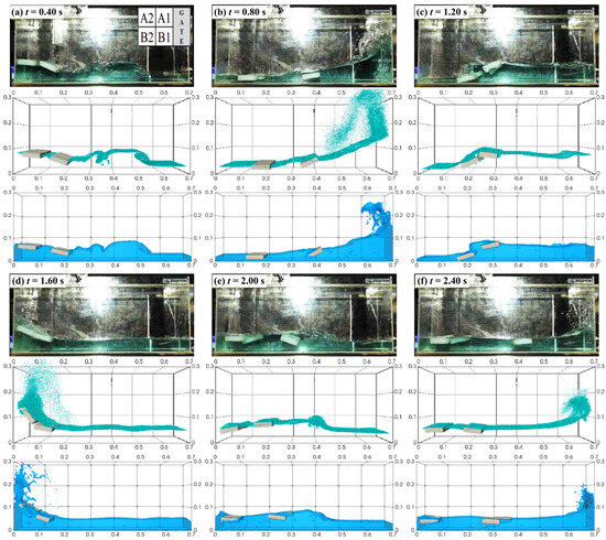
Figure 2.
Snapshots of the TC4-2.5 at time intervals of (a) t = 0.4 s, (b) t = 0.8 s, (c) t = 1.2 s, (d) t = 1.6 s, (e) t = 2.0 s, and (f) t = 2.4 s. Each subfigure comprises three images: the top is the laboratory TC result, the middle is TC4-N by Amaro et al. [31], and the bottom image illustrates the results from the current numerical model.

Figure 3.
Snapshots of the TC9-2.5 at time intervals of (a) t = 0.4 s, (b) t = 0.8 s, (c) t = 1.2 s, (d) t = 1.6 s, (e) t = 2.0 s, and (f) t = 2.4 s. Each subfigure comprises three images: the top is the laboratory TC result, the middle is TC9-N by Amaro et al. [31], and the bottom image illustrates the results from the current numerical model.
In TC4-2.5, at the instant t = 0.40 s, the wavefront travels smoothly downstream and impacts the downstream wall. However, the presence of the initial downstream fluid layer significantly alters the flow behavior. As depicted in Figure 2 (refer also to the Supplementary Material Figures S1–S4), the downstream fluid remains unaffected by the wave, resulting in the formation of a mushroom-like jet, as previously reported by Stansby et al. [58] and M. Jánosi et al. [59]. At t = 0.8 s, a backward wave or fluid run-up is generated in these cases, subsequently moving towards the upstream wall. By t = 1.60 s, the wave moves back to the downstream wall after hitting the upstream wall, creating a flow run-up. Regarding the positioning of the blocks, when the gate opens, the current numerical model indicates that blocks A1 and B1 move slightly faster than observed in the laboratory TC results. As the wave rebounds from both the upstream and downstream walls, the blocks in the current numerical model exhibit more pronounced differences compared to the laboratory TC. Such discrepancies are expected given the challenging and chaotic nature of the phenomena over time, including breaking waves, wave splash, and plunging jets. Similar behavior is observed in the results from the TC4-N [31]. A qualitative comparison of the free-surface profiles and block positioning between the current numerical model and the laboratory TC results indicates that the current numerical model has successfully reproduced the dam-break flow behavior across all the TC4 scenarios.
Results for TC9-2.5 are shown in Figure 3 and the rest of TC9 simulations are presented in Supplementary Material (Figures S5–S8). A reasonable agreement was observed between the current numerical simulation results and the laboratory experiments of TC9 from when the gate opened, and the blocks were released up until t = 1.2 s. Afterward, the convergence of the collapsing upward water flow and the reflected wave significantly disturbed the water surface, resulting in more chaotic motion of the solids, particularly those downstream.
Early in the simulation at t = 0.40 s, the formation of a mushroom-like jet occurs when a downstream fluid layer is present. At the instants t = 0.8 s and t = 1.60 s, an increase in the downstream fluid layer leads to slower wave propagation. In other words, events such as wave impact and run-up occur later as the depth of the downstream fluid increases. Similar observations were reported in the results of TC9-N derived by Amaro et al. [31].
The results of the current numerical simulation indicated that in the TC9-0.0 and TC9-1.0, the last row of blocks adhered to the bottom of the tank and did not float back up after the wave rebounded from the downstream wall (Figures S5 and S6). This issue can be attributed to the characteristics of mesh-based numerical models. When the water height beneath the blocks drops below one cell size, the blocks adhere to the bottom, and there is no uplift force to cause the blocks to float again. Refining the mesh may or may not solve this problem, depending on the nature of the issue. As expected, this issue was resolved when the downstream water level was increased in TC9-2.5 and TC9-5.0 (Figures S7 and S8) and wasn’t noted in the numerical results of TC9-N conducted by Amaro et al. [31].
Figure 4 and Figure 5 display snapshots of the TC25-PP and TC25-I, respectively with their associated numerical simulation results of TC25-N by Billy et al. [33] and current numerical simulation results at different times.
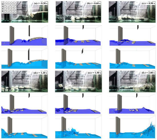
Figure 4.
Snapshots of the TC25-PP at time intervals of (a) t = 0.3 s, (b) t = 0.6 s, (c) t = 0.9 s, (d) t = 1.2 s, (e) t = 1.5 s, and (f) t = 2.0 s. Each subfigure comprises three images: the top is the laboratory TC result, the middle is TC25-N by Billy et al. [33], and the bottom image illustrates the results from the current numerical model.

Figure 5.
Snapshots of the TC25-I at time intervals of (a) t = 0.3 s, (b) t = 0.6 s, (c) t = 0.9 s, (d) t = 1.2 s, (e) t = 1.5 s, and (f) t = 2.0 s. Each subfigure comprises three images: the top is the laboratory TC result, the middle is TC25-N by Billy et al. [33], and the bottom image illustrates the results from the current numerical model.
Following the gate’s removal, a dam-break wave forms and carries the blocks downstream until it encounters the ICS (around 0.9 s). Most of the blocks are obstructed by the ICS, as the blocks are larger than the spaces between the ICS. However, a few blocks rotate and pass through these gaps. There is good overall agreement between the laboratory TC results and current numerical wave profiles and blocks’ positions. In TC25-PP, the wave in the current numerical model propagates slightly faster than in the experiment (Figure 4). This minor discrepancy arises from the constant gate removal speed used in the numerical model, whereas in the laboratory TC, variations occur due to the gate’s friction against the tank’s lateral walls. A complete discussion about the vertical gate speed can be found in Amaro et al. [31]. Slight variations are also observed between laboratory TC’s repetitions, which relate to the chaotic nature of the experiment. For example, in the laboratory snapshot of Figure 4a, block 21 (See Figure 1d) flips at 0.3 s due to friction with the gate, a detail not replicated in the current numerical results. Similar behavior was reported also in the numerical simulation results of TC25-N by Billy et al. [33].
The set of laboratory TC results demonstrates that the last row of blocks (i.e., blocks 5, 10, 15, 20, 25 as shown in Figure 1d are transported downstream, although their motion is much slower in the current numerical simulations for both real ice and PP materials. In the current numerical model, this row of blocks moves faster compared with in the results of simulated model in TC25-N [33], but their movement is still slower than observed in the laboratory TC results. The snapshots at t = 1.2, and 1.5 s display the reflected wave after it hits the downstream tank face. Wave splashes from the reflected wave impacting the ICS can be seen in the laboratory TC experiments and the current numerical model but not in the numerical model results of TC25-N [33]. This feature is captured more effectively by the current numerical model due to the use of the TruVOF method within the framework numerical model. The latter snapshot (Figure 4f) indicates that the wave intensity is very similar between the current numerical model and the laboratory TC results and is slightly higher in the laboratory TC results compared to the model results of TC25-N [33], yet the current numerical model achieves sufficient accuracy.
Regarding Figure 5, the current numerical model generally captured the main features of the laboratory TC. Real ice tended to adhere together more, as observed at t = 0.9, 1.2, and 1.5 s (Figure 5c–e). However, similar to the TC25-N of Billy et al. [33], the current numerical model could not capture this feature. The reverse wave and the resulting splash, due to the presence of the ICS, were captured with sufficient accuracy (Figure 5e). Additionally, the current numerical model showed better agreement in simulating the results compared to TC25-N and the laboratory test case results when the reverse wave reached the upstream wall at t = 2.0 s (Figure 5f).
Some laboratory experiments in a straight channel, based on the work of Billy et al. [33], involving 160 blocks under varying flow conditions (Froude numbers) and block materials (real ice and PP) with ICS were tested to examine the capabilities of the current simulation model with more complex characteristics. Unfortunately, the current numerical model became unstable and failed to converge. It should be noted that, despite the software’s indication that it can handle up to 500 moving and non-moving objects [46], the graphical platform became sluggish with more than 50 blocks. Furthermore, although shapes can be defined by the software and imported using (.stl) files, each block must be defined separately to have 6-DOF. As this software is commercial software, the authors could not verify the exact underlying cause of these issues. Factors such as advection-diffusion, turbulence, the chaotic nature of block interactions with each other and the ICS, and the coupling of the solid phase algorithm with the fluid phase could contribute to these instabilities. These laboratory experiments in long channel and related aspects are suggested for future investigation.
3.2. Accuracy of Simulations
To quantify the accuracy of the results obtained from the current numerical model compared to the laboratory TC and TC-N conducted by Amaro et al. [31] and Billy et al. [33], the longitudinal (x direction) and vertical (z direction) motions of different blocks were tracked and plotted. For the TC4-2.5 and TC9-2.5 scenarios, the longitudinal and vertical motions of blocks B1 and B2, and blocks C1, C2, and C3 are plotted in Figure 6 and Figure 7 respectively. Similar plots for the rest of the TC4 and TC9 scenarios are included in the Supplementary Material Figures S9–S16. It should be noted that the data for the laboratory TC and the TC4-N/TC9-N were extracted from Amaro et al. [31].
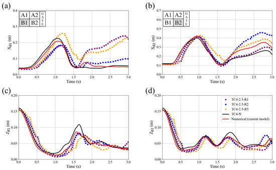
Figure 6.
Comparison of the trajectory of the blocks from the laboratory experiment TC4-2.5 (different lines refer to the results of the different repetitions of the experiments TC4-2.5-R1, TC4-2.5-R2, and TC4-2.5-R3) with TC4-N from Amaro et al. [31] and the current numerical model for the x-direction of (a) block B1 and (b) block B2 and along the z-direction for (c) block B1 and (d) block B2.
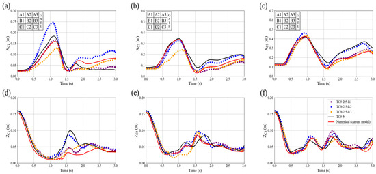
Figure 7.
Comparison of the trajectory of the blocks from the laboratory experiment TC9-2.5 (different lines refer to the results of the different repetitions of the experiments TC9-2.5-R1, TC9-2.5-R2, and TC9-2.5-R3) with TC9-N from Amaro et al. [31] and the current numerical model for the x-direction of (a) block C1, (b) block C2 and (c) block C3, and along the z-direction for (d) block C1, (e) block C2 and (f) block C3.
Regarding TC4-2.5, the simulated motion of the blocks generally follows the same trends observed in the laboratory TC. Looking at Figure 6a,b, the results of the current numerical model show that at around t = 1.0 s, approximately 0.2 s after the reverse wave begins generating, both blocks B1 and B2 reach their maximum movement in the x direction. Subsequently, when the reverse wave hits the blocks, they both move toward the downstream wall until t = 1.5 s. Figure 6c,d, illustrates that both the current numerical model and TC4-N correctly capture the wave amplitude. Comparing the results of the current numerical model and TC4-N [31] reveals a similar tendency in simulating scenarios with 4 blocks across both numerical models (Figure 6). In TC4-0.0 (Figure S9), by around 1.2 s, current numerical model results tend to overestimate the motion of block B1 in the x-direction. This discrepancy may be due to challenges in setting the initial arrangement of the blocks in regular, equally spaced positions, which could lead to values that differ from those computed numerically. Additionally, variations in the gate removal process may also affect the motions. An average gate removal speed of 0.4 m/s was assumed based on the results from Amaro et al. [31]. A similar issue was also reported in the TC4-N when dealing with these scenarios [31].
In all numerical simulations results of TC, after t = 1.5 s, block B1 is propelled by the reflected wavefront, leading to larger discrepancies between the current numerical simulation and laboratory TC results. A similar pattern was observed in the simulation results for block B2 as well. These discrepancies, which also appear between laboratory repetition, are understandable given the chaotic nature of this stage. This chaos is due to an intense splash created by the vertical run-up jet falling onto the underlying fluid, mixing air with water as reported by Amaro et al. [31]. In fact, processes such as wave-splash, plunging jet penetration, and breaking waves typically exhibit chaotic behaviors, as extensively documented through laboratory observations and numerical simulations in Wei et al. [60]. Similar scenarios were observed in the laboratory TC with varying water levels downstream, but the noted differences between simulated values compared to laboratory values generally decrease with the increase of water depth downstream.
Similar to TC4-2.5, the current numerical simulations for TC9-2.5 generally follow the same trends observed in the laboratory experiments. Comparing the results of the current numerical model and TC9-N [31] reveals a similar tendency in simulating scenarios with 9 blocks across both models (Figure 7). For the TC9-0.0 and TC9-1.0 cases, the last row of blocks—specifically C1 as a representative—tends to stick to the bottom of the tank after the downstream wave travels upstream, as shown in the Supplementary Material Figures S13 and S14. A similar movement trend of block C1 was also observed in the TC9-N by Amaro et al. [31]. Similar to the TC4, the fluid flow becomes chaotic at this stage, with solid motions influenced by factors such as wave breaking and multiple solid collisions. Overall, the current numerical simulations demonstrated better agreement in simulating the motion of block C3 in the x-direction compared to blocks C1 and C2. In the z direction, except for the two previously mentioned cases, although the numerical simulations show some local discrepancies when compared with laboratory TC results, the overall characteristics of the vertical motions are well captured by the numerical models.
The RMSE for TC4 and TC9 is presented in Figure 8. For TC4, both numerical models result demonstrate comparable accuracy in simulating block movements in the z-direction with an average RMSE of 0.0114 for current numerical model and 0.0116 for TC4-N. In the x-direction, the accuracy decreases with an average RMSE of 0.0572 for current numerical model and 0.0635 for TC4-N (see Figure 8a). Neither model results exhibit a consistent trend relative to the water level downstream and both show reduced accuracy at TC4-2.5, especially in simulating motion in the X direction, with RMSE values of 0.0650 for current numerical model and 0.0791 for TC4-N. Considering all TC4 across both directions, current numerical model performed better in TC4-5.0 with an RMSE of 0.0313, while simulated numerical results of TC4-N by Amaro et al. [31] excelled in TC4-1.0, achieving an RMSE of 0.0263. Overall, both the current numerical model and TC4-N exhibit sufficient accuracy in handling TC4, with the current numerical model achieving an overall RMSE of 0.0418, and TC4-N recording an RMSE of 0.0472.
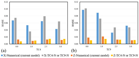
Figure 8.
RMSE for numerical simulation results in the x and z directions comparing the accuracy of the current model with TC4-N and TC9-N for (a) TC4, and (b) TC9, respectively.
For TC9, a general decreasing trend in RMSE with increasing water depth downstream was observed in the accuracy of TC9-N and the current numerical model results, with the exception of the RMSE for the current numerical model for TC9-2.5 being smaller than that of TC9-5.0 (see Figure 8b). Current numerical model results were less accurate (higher RMSE) in the x-direction for the TC9-1.0 and TC9-5.0 when compared to TC9-N. However, the accuracy of current model simulations at TC9-2.5 was considerably higher than TC9-N, with RMSE values of 0.0324 and 0.0124 in the x and z directions, respectively. Overall, both the current numerical model and TC9-N demonstrate sufficient accuracy in handling TC9, with an overall average RMSE of 0.0527, and 0.0507 respectively.
Comparing the accuracy of the results of the current numerical model with TC4-N and TC9-N, it was found that the current numerical model achieves more accurate results in for the TC4 (4 blocks) cases compared to the TC9 (9 blocks) cases.
For TC25-PP and TC25-I, the trajectories of blocks C6 and C12 in the x-direction, and C21 and C22 in the z-direction are plotted in Figure 9 and Figure 10 respectively. The tracking of block positions shows generally good agreement between the laboratory TC and both the current numerical model and the TC25-N results. The trajectories indicate that block positions are highly correlated with free-surface waves (dam-break and return waves) in TC25-N, although the return wave was better simulated in the current numerical model. For example, block C6 in TC25-PP (Figure 9a) in the current numerical model, hits the ICS and then passes it reaching a maximum distance of 0.41 m. However, when the wave returns from the downstream wall, this block becomes jammed downstream of the ICS, causing its trajectory to stall at a distance of about 0.33 m. This issue in the current numerical model maybe can be resolved by refining the mesh. However, the chaotic nature of the phenomena, and the increase in computational time required for refining the mesh is significant enough that this flaw may be deemed acceptable. A similar issue was observed in the trajectory in the z-direction of the TC25-N results of block C21 (Figure 10c). The block remained in the same depth once it hit the ICS and couldn’t move with the returning wave. Regarding Figure 10a, the results of the current numerical model show that until t = 0.7 s, the model closely captures the movement of block C6 compared to the laboratory TC. After this time, some discrepancies are observed, likely due to the chaotic nature of the phenomenon. It should be noted that this block is in the first row, and factors such as gate speed and friction between the block and the gate can significantly impact the results. On the other hand, Figure 10b shows that the results of the current numerical model are more accurate compared to TC25-N by Billy et al. [33] after t = 1.5 s. Regarding the movement in the z-direction and Figure 10c,d, both the current model and TC25-N correctly capture the main features at the earlier stage. Following this, discrepancies can be observed due to the chaotic nature of the phenomenon. These differences were also observed in the repetitions of the laboratory test case and reported by Billy et al. [33], indicating that they are unavoidable. Like in the TC4 and TC9, the numerical models perform better in simulating movement in the z-direction. Overall, the main features of the blocks’ movements were well captured in the current numerical model.
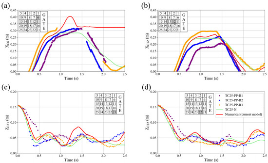
Figure 9.
Comparison of the trajectory of the blocks from the laboratory experiment TC25-PP (different lines refer to the results of the different repetitions of the experiments TC25-PP-R1, TC25-PP-R2, and TC25-PP-R3) with TC25-N from Billy et al. [33] and the current numerical model for the x-direction of (a) block C6 and (b) block C12, and along the z-direction for (c) block C21 and (d) block C22.
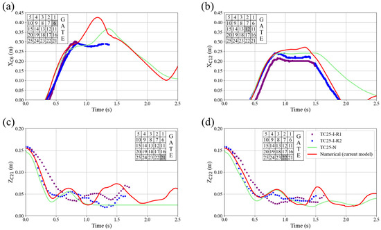
Figure 10.
Comparison of the trajectory of the blocks from the laboratory experiment TC25-I (different lines refer to the results of the different repetitions of the experiments TC25-I-R1, and TC25-I-R2) with TC25-N from Billy et al. [33] and the current numerical model for the x-direction of (a) block C6 and (b) block C12, and along the z-direction for (c) block C21 and (d) block C22.
The RMSE for the trajectory of the blocks in the x- and z-direction for TC25-PP and TC25-I for the current numerical model and TC25-N is illustrated in Figure 11. The RMSE for the x-direction in TC25-PP shows that the current numerical model performs slightly better than the TC25-N with a RMSE of 0.0953, while that for the TC25-N is 0.1081. The same performance is shown for the TC25-I with lower values for the RMSE of 0.0552 and 0.0704 for the current model and TC25-N, respectively. The overall RMSE in both x- and z-direction is 0.0753 and 0.0860 for the current numerical model and TC25-N, respectively. Both models performed better for the TC25-I with an overall RMSE of 0.0441 and 0.0557 for the current numerical model and TC25-N, respectively. The higher values of the RMSE for TC25-PP as opposed to TC25-I arises from the fact that block C6 in the current numerical model and block C16 in the TC25-N became jammed downstream of the ICS when the return wave hit the ICS. This phenomenon was not observed in the TC25-I simulation results, which highlight the benefits and importance of using real ice material properties in the simulations.
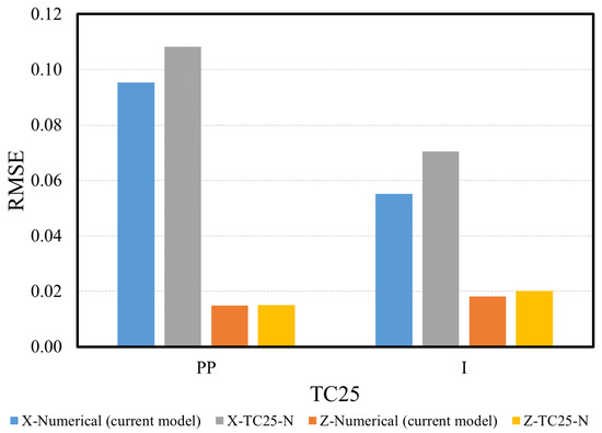
Figure 11.
RMSE for numerical simulation results in the x and z directions comparing the accuracy of the current model with TC25-N for the TC25 experiments for polypropylene (PP) and ice (I) blocks.
3.3. Computational Efficiency
Computational efficiency refers to the performance of algorithms or systems in terms of resource utilization, processing time, and scalability. While current numerical model, and the models used for TC4-N/TC9-N and TC25-N by Amaro et al. [31] and Billy et al. [33], respectively, process different algorithms, to provide a clearer understanding of computational time, the computational cost of each model is reported in Table 2.
Table 2.
Computational performance of numerical models.
The numerical model used in TC25-N by Billy et al. [33] is based on the DEM-SPH method. The DEM method is used to address the solid motion and interaction, while the SPH method is used to solve the fluid conservation equations. The coupling of the two methods is presented in Canelas et al. [61]. The most time-consuming aspect of this model involves calculating contacts between solids. The Lagrangian methods require a large number of particles and have time step restrictions to ensure stability, which incurs high computational costs. However, these costs can be reduced by optimizing the parallelization of the code [32]. A GPU-accelerated version of this model was used in studies by Billy et al. [32,33], and more information about CPU and GPU implementations of the code is detailed in Domínguez et al. [62]. Different computational performances were recorded regarding the available resources for simulating the TC25-N by Billy et al. [33] and is reported in Table 2.
The numerical model used in TC4-N/TC9-N by Amaro et al. [31], is based on the MPS and DEM methods are used to solve the governing equations of the continuum phase (water) and discrete phase (solid ice blocks), respectively. Like other particle-based methods, the DEM-MPS method also suffers from high computational costs associated with the large number of particles required to address large-scale practical engineering problems. The results for TC4-N and TC9-N were obtained using parallel computing in shared memory systems using OpenMP® 3.0 [63] to simulate these cases within a reasonable processing time [31]. Although Amaro et al. [31] did not distinguish the computational performance of this particle method for TC4-N and TC9-N, they reported a range for it, as shown in Table 2.
On the other hand, the current numerical model operates within a Eulerian framework. Factors such as the size of each cell, which determines the number of cells used, parameters to be simulated (e.g., GMO), and the number of cores provided by the software license, dictate the speed of the simulation. In Table 2, simulations were conducted on various machines, including personal computers, the HPC server of Computational Hydrosystems Lab (CHLab) at Polytechnique Montreal, and a Compute Canada server. It should be noted that the computational times for the numerical models results of TC4-N/TC9-N and TC25-N are sourced from Amaro et al. [31] and Billy et al. [33], and the physical simulation time for laboratory TC was 3 s.
4. Conclusions
In this study, the FLOW-3D numerical model (referred to as “current numerical model”) was evaluated to determine its capability to simulate ice blocks movements using the GMO module. The accuracy and efficiency of the numerical model were also investigated by comparing results with laboratory experiments TC and other numerical models (conducted by others) across dam break scenarios with varying numbers of blocks, materials, and the presence or absence of an ICS. The following is a summary of the conclusions drawn from the current study:
- -
- The current numerical model which is a structured mesh-based model, has a user-friendly graphical interface that can model a wide range of hydraulic problems, which is its primary advantage. On the other hand, meshless methods are particularly well-suited for handling complex conditions without the need for a predefined grid, offering greater flexibility in defining material properties and setting up simulations with high accuracy, such as simulating the jamming of blocks behind an ICS. However, these methods can be more challenging to configure. Moreover, meshless models often make more efficient use of computational resources by leveraging GPU acceleration, in contrast to commercial software like the current numerical model, which is typically constrained to CPU processing and the number of cores available under the license. For instance, the computational time for TC25 using a meshless method, as conducted by Billy et al. [33] was approximately 1.5 h, compared to nearly 33 h required by the current numerical model.
- -
- Comparing the qualitative results through the snapshots of the current numerical model and the laboratory TC shows that the current numerical model can accurately capture the main features of the dam breaking, such as the reverse wave and the breaking of the reverse wave. Additionally, the current numerical model produces acceptable results when adding complexity to the cases, such as incorporating floating blocks, increasing the downstream water level, and adding ICS to the tank.
- -
- The results also indicated that the current numerical model could accurately reproduce the movement of blocks in simple dam break cases with varying numbers of blocks and downstream water levels, both with and without an ICS. An RMSE of 0.0418 and 0.0527 was obtained for the current numerical model when dealing with 4 and 9 blocks with different downstream water levels, respectively.
- -
- For the 25 blocks cases with an ICS, the current numerical model showed an RMSE of 0.0441 and 0.0753, for the real and artificial ice blocks, respectively. The lower accuracy is due to the jamming of the block downstream of the ICS when the reverse wave comes back from the upstream wall of the tank. Moreover, the simulation accuracy of real ice blocks (RMSE) is enhanced compared to artificial blocks, therefore, it is essential to define the material properties correctly to obtain correct results, especially in real ice simulations.
- -
- In general, both, the current numerical model and the meshless models were more accurate in reproducing the trajectory of blocks in the z-direction compared to the x-direction. Nevertheless, the current numerical model was slightly more accurate with an average overall RMSE of 0.0534 from all cases (and directions), compared to an average RMSE of 0.0599 for the meshless models.
- -
- Although the current numerical model exhibited a similar computational time (ranging from 25 to 40 h for 3 s of physical time) to the particle method numerical model conducted by Amaro et al. [31], constraints on the number of cores available for use by the processors (depending on the license type) and reliance on CPU processing resulted in greater resource consumption.
- -
- The use of sophisticated mesh techniques, such as nested meshes, not only reduced computational time but also diminished the accuracy of the results. Therefore, a single mesh block was recommended based on the recommendations of the software manual. Like other mesh-based methods, refining the mesh in the current numerical model could enhance accuracy but increases computational time.
- -
- The current numerical model did not converge and became unstable when dealing with more complex phenomena, such as jamming several blocks behind an ICS in a straight channel. This problem could be related to numerous factors, including the chaotic nature of the phenomena, the embedded collision model, the coupling of the solid and fluid phases, among others. These aspects are suggested topics for future investigation.
As a summary, it is recommended to test newer versions of the current numerical model to determine if it can simulate the more complex phenomena of block jamming with increased number of blocks. It is also suggested that the particle methods model be further developed to handle simulations of real-scale ice dynamic problems involving a large number of ice floes, such as ice-jam formation, breakup, and interactions with hydraulic structures. This includes improving the resolution of particle interactions, integrating detailed ice mechanics, and coupling particle methods with high-fidelity hydrodynamic models. Additionally, developments in computational efficiency and scalability are crucial to handle large-scale simulations effectively. Future studies should also consider a numerical model capable of simulating internal ice stress and the ice-breaking processes and coupling them with 3D hydrodynamic flow.
Supplementary Materials
The following supporting information can be downloaded at: https://www.mdpi.com/article/10.3390/w16172454/s1, Figure S1: Snapshots of the TC4-0.0 at time intervals of (a) t = 0.4 s, (b) t = 0.8 s, (c) t = 1.2 s, (d) t = 1.6 s, (e) t = 2.0 s, and (f) t = 2.4 s. Each subfigure comprises three images: the top is the laboratory TC result, the middle is TC4-N by Amaro et al. [31], and the bottom image illustrates the results from the current numerical model; Figure S2: Snapshots of the TC4-1.0 at time intervals of (a) t = 0.4 s, (b) t = 0.8 s, (c) t = 1.2 s, (d) t = 1.6 s, (e) t = 2.0 s, and (f) t = 2.4 s. Each subfigure comprises three images: the top is the laboratory TC result, the middle is TC4-N by Amaro et al. [31], and the bottom image illustrates the results from the current numerical model; Figure S3: Snapshots of the TC4-2.5 at time intervals of (a) t = 0.4 s, (b) t = 0.8 s, (c) t = 1.2 s, (d) t = 1.6 s, (e) t = 2.0 s, and (f) t = 2.4 s. Each subfigure comprises three images: the top is the laboratory TC result, the middle is TC4-N by Amaro et al. [31], and the bottom image illustrates the results from the current numerical model; Figure S4: Snapshots of the TC4-5.0 at time intervals of (a) t = 0.4 s, (b) t = 0.8 s, (c) t = 1.2 s, (d) t = 1.6 s, (e) t = 2.0 s, and (f) t = 2.4 s. Each subfigure comprises three images: the top is the laboratory TC result, the middle is TC4-N by Amaro et al. [31], and the bottom image illustrates the results from the current numerical model; Figure S5: Snapshots of the TC9-0.0 at time intervals of (a) t = 0.4 s, (b) t = 0.8 s, (c) t = 1.2 s, (d) t = 1.6 s, (e) t = 2.0 s, and (f) t = 2.4 s. Each subfigure comprises three images: the top is the laboratory TC result, the middle is TC9-N by Amaro et al. [31], and the bottom image illustrates the results from the current numerical model; Figure S6: Snapshots of the TC9-1.0 at time intervals of (a) t = 0.4 s, (b) t = 0.8 s, (c) t = 1.2 s, (d) t = 1.6 s, (e) t = 2.0 s, and (f) t = 2.4 s. Each subfigure comprises three images: the top is the laboratory TC result, the middle is TC9-N by Amaro et al. [31], and the bottom image illustrates the results from the current numerical model; Figure S7: Snapshots of the TC9-2.5 at time intervals of (a) t = 0.4 s, (b) t = 0.8 s, (c) t = 1.2 s, (d) t = 1.6 s, (e) t = 2.0 s, and (f) t = 2.4 s. Each subfigure comprises three images: the top is the laboratory TC result, the middle is TC9-N by Amaro et al. [31], and the bottom image illustrates the results from the current numerical model; Figure S8: Snapshots of the TC9-5.0 at time intervals of (a) t = 0.4 s, (b) t = 0.8 s, (c) t = 1.2 s, (d) t = 1.6 s, (e) t = 2.0 s, and (f) t = 2.4 s. Each subfigure comprises three images: the top is the laboratory TC result, the middle is TC9-N by Amaro et al. [31], and the bottom image illustrates the results from the current numerical model; Figure S9: Comparison of the trajectory of the blocks from the laboratory experiment TC4-0.0 (different lines refer to the results of the different repetitions of the experiments TC4-0.0-R1, TC4-0.0-R2, and TC4-0.0-R3) with TC4-N from Amaro et al. [31] and the current numerical model for the x-direction of (a) block B1 and (b) block B2 and along the z-direction for (c) block B1 and (d) block B2; Figure S10: Comparison of the trajectory of the blocks from the laboratory experiment TC4-1.0 (different lines refer to the results of the different repetitions of the experiments TC4-1.0-R1, TC4-1.0-R2, and TC4-1.0-R3) with TC4-N from Amaro et al. [31] and the current numerical model for the x-direction of (a) block B1 and (b) block B2 and along the z-direction for (c) block B1 and (d) block B2; Figure S11: Comparison of the trajectory of the blocks from the laboratory experiment TC4-2.5 (different lines refer to the results of the different repetitions of the experiments TC4-2.5-R1, TC4-2.5-R2, and TC4-2.5-R3) with TC4-N from Amaro et al. [31] and the current numerical model for the x-direction of (a) block B1 and (b) block B2 and along the z-direction for (c) block B1 and (d) block B2; Figure S12: Comparison of the trajectory of the blocks from the laboratory experiment TC4-5.0 (different lines refer to the results of the different repetitions of the experiments TC4-5.0-R1, TC4-5.0-R2, and TC4-5.0-R3) with TC4-N from Amaro et al. [31] and the current numerical model for the x-direction of (a) block B1 and (b) block B2 and along the z-direction for (c) block B1 and (d) block B2; Figure S13: Comparison of the trajectory of the blocks from the laboratory experiment TC9-0.0 (different lines refer to the results of the different repetitions of the experiments TC9-0.0-R1, TC9-0.0-R2, and TC9-0.0-R3) with TC9-N from Amaro et al. [31] and the current numerical model for the x-direction of (a) block C1, (b) block C2 and (c) block C3, and along the z-direction for (d) block C1, (e) block C2 and (f) block C3; Figure S14: Comparison of the trajectory of the blocks from the laboratory experiment TC9-1.0 (different lines refer to the results of the different repetitions of the experiments TC9-1.0-R1, TC9-1.0-R2, and TC9-1.0-R3) with TC9-N from Amaro et al. [31] and the current numerical model for the x-direction of (a) block C1, (b) block C2 and (c) block C3, and along the z-direction for (d) block C1, (e) block C2 and (f) block C3; Figure S15: Comparison of the trajectory of the blocks from the laboratory experiment TC9-2.5 (different lines refer to the results of the different repetitions of the experiments TC9-2.5-R1, TC9-2.5-R2, and TC9-2.5-R3) with TC9-N from Amaro et al. [31] and the current numerical model for the x-direction of (a) block C1, (b) block C2 and (c) block C3, and along the z-direction for (d) block C1, (e) block C2 and (f) block C3; Figure S16: Comparison of the trajectory of the blocks from the laboratory experiment TC9-5.0 (different lines refer to the results of the different repetitions of the experiments TC9-5.0-R1, TC9-5.0-R2, and TC9-5.0-R3) with TC9-N from Amaro et al. [31] and the current numerical model for the x-direction of (a) block C1, (b) block C2 and (c) block C3, and along the z-direction for (d) block C1, (e) block C2 and (f) block C3.
Author Contributions
Conceptualization: H.P., T.G. and A.S.; Formal analysis: H.P., T.G. and A.S.; Investigation: H.P., T.G. and A.S.; Methodology: H.P., T.G. and A.S.; Project administration: T.G.; Resources: T.G. and A.S.; Software: H.P.; Supervision: T.G. and A.S.; Validation: T.G. and A.S.; Visualization: H.P., T.G. and A.S.; Writing—original draft: H.P.; Writing—review & editing: T.G. and A.S. All authors have read and agreed to the published version of the manuscript.
Funding
This research project was supported by the Ministère de Sécurité Publique de Québec (MSP) under the FLUTEIS project (project number CPS 18-19-26). Some part of FLOW-3D® V.2023 R1 software made available through the FLOW-3D Academic Program.
Data Availability Statement
The data presented in this study are available on request from the corresponding author due to privacy.
Acknowledgments
The authors would like to thank Jonathan Bouchard and Cristine Webb from Flow Science, Inc. for their continuous support and collaboration. The authors would like to express their sincere gratitude for the invaluable comments provided by the reviewers and editor.
Conflicts of Interest
The authors declare no conflicts of interest.
References
- Perham, R.E. Ice Sheet Retention Structures; Cold Regions Research and Engineering Lab: Hanover, NH, USA, 1983. [Google Scholar]
- Tuthill, A.M. Structural Ice Control: Review of Existing Methods; Cold Regions Research & Engineering Laboratory, U.S. Army Corps of Engineers: Hanover, NH, USA, 1995. [Google Scholar]
- Beltaos, S. Progress in the Study and Management of River Ice Jams. Cold Reg. Sci. Technol. 2008, 51, 2–19. [Google Scholar] [CrossRef]
- Hicks, F.E. An Introduction to River Ice Engineering: For Civil Engineers and Geoscientists; CreateSpace Independent Publishing Platform: Charleston, SC, USA, 2016; ISBN 978-1-4927-8863-8. [Google Scholar]
- Beltaos, S. Hydrodynamic Characteristics and Effects of River Waves Caused by Ice Jam Releases. Cold Reg. Sci. Technol. 2013, 85, 42–55. [Google Scholar] [CrossRef]
- Benin, W.J.; Ghobrial, T.; Pourshahbaz, H.; Pierre, A. Characterization of Ice Retention during Breakup Upstream of an Ice Control Structure Using a Juxtaposed Camera System. In Proceedings of the 27th IAHR International Symposium on Ice, Gdańsk, Poland, 9–13 June 2024. [Google Scholar]
- Pourshahbaz, H.; Ghobrial, T.; Shakibaeinia, A. Field Monitoring of River Ice Processes in the Vicinity of Ice Control Structures in the Province of Quebec, Canada. Can. J. Civ. Eng. 2024, 51, 200–214. [Google Scholar] [CrossRef]
- Ouranos. Vers L’adaptation Synthèse des Connaissances sur les Changements Climatiques au Québec; Ouranos: Montreal, QC, Canada, 2015; ISBN 978-2-923292-18-2. [Google Scholar]
- Lafleur, C.; Nolin, S.; Pelletier, P.; Babineau, L. Understanding, Monitoring and Preventing Ice-Jam Flooding on an Urban River in the Quebec City Area. In Proceedings of the 21st Workshop on the Hydraulics of Ice Covered Rivers, Saskatoon, SK, Canada, 29 August–1 September 2021; p. 12. [Google Scholar]
- Lever, J.H.; Gooch, G. Performance of a Sloped-Block Ice-Control Structure in Hardwick, VT. In Proceedings of the 13th Workshop on the Hydraulics of Ice Covered Rivers, Hanover, NH, USA, 15–16 September 2005; p. 7. [Google Scholar]
- Lever, J.H.; Gooch, G. Cazenovia Creek Ice Control Structure: A Comparison of Two Concepts. In Proceedings of the 10th Workshop on the Hydraulics of Ice Covered Rivers, Winnipeg, MB, Canada, 8–11 June 1999. [Google Scholar]
- Lever, J.H.; Gooch, G. Design of Cazenovia Creek Ice Control Structure. J. Cold Reg. Eng. 2001, 15, 103–124. [Google Scholar] [CrossRef]
- Kolerski, T.; Shen, H.T.; Liu, L. DynaRICE Modeling to Assess the Performance of an Ice Control Structure on the Lower Grasse River. In Proceedings of the 19th IAHR International Symposium on Ice, Vancouver, BC, Canada, 6–11 July 2008. [Google Scholar]
- Carr, M.; Tuthill, A.M.; Vuyovich, C.M. Dam Removal Ice Hydraulic Analysis and Ice Control Alternatives. In Proceedings of the 16th Workshop on River Ice, Winnipeg, MB, Canada, 18–22 September 2011. [Google Scholar]
- Nolin, S.; Pelletier, P.; Groux, F. Modelling the Impacts of Dam Rehabilitation on River Ice Jam: A Case Study on the Matane River, QC, Canada. In Proceedings of the 19th Workshop on the Hydraulics of Ice Covered Rivers, Whitehorse, YT, Canada, 9–12 July 2017; p. 12. [Google Scholar]
- Hatta, M.P.; Widyastuti, I.; Makkarumpa, A.M.M. The Effect of Triangle Slope Variation on Froude Number with Numerical Simulation. Civ. Eng. J. 2023, 9, 3136–3146. [Google Scholar] [CrossRef]
- Pu, J.H.; Wallwork, J.T.; Khan, M.A.; Pandey, M.; Pourshahbaz, H.; Satyanaga, A.; Hanmaiahgari, P.R.; Gough, T. Flood Suspended Sediment Transport: Combined Modelling from Dilute to Hyper-Concentrated Flow. Water 2021, 13, 379. [Google Scholar] [CrossRef]
- U.S. Army Corps of Engineers HEC-RAS River Analysis System. Hydraulic Reference Manual, Version 5.0; Institute of Water Resources, Hydrologic Engineering Center: Davis, CA, USA, 2016.
- Shen, H.T.; Wang, D.S.; Lal, A.M.W. Numerical Simulation of River Ice Processes. J. Cold Reg. Eng. 1995, 9, 107–118. [Google Scholar] [CrossRef]
- Lindenschmidt, K.-E. RIVICE—A Non-Proprietary, Open-Source, One-Dimensional River-Ice Model. Water 2017, 9, 314. [Google Scholar] [CrossRef]
- Shen, H.T.; Su, J.; Liu, L. SPH Simulation of River Ice Dynamics. J. Comput. Phys. 2000, 165, 752–770. [Google Scholar] [CrossRef]
- Shen, H.T. Mathematical Modeling of River Ice Processes. Cold Reg. Sci. Technol. 2010, 62, 3–13. [Google Scholar] [CrossRef]
- Cundall, P.A.; Strack, O.D.L. A Discrete Numerical Model for Granular Assemblies. Géotechnique 1979, 29, 47–65. [Google Scholar] [CrossRef]
- Tuhkuri, J.; Polojärvi, A. A Review of Discrete Element Simulation of Ice–Structure Interaction. Phil. Trans. R. Soc. A 2018, 376, 20170335. [Google Scholar] [CrossRef] [PubMed]
- Daly, S.; Hopkins, M. Estimating Forces on an Ice Control Structure Using DEM. In Proceedings of the 11th Workshop on the Hydraulics of Ice Covered Rivers, Ottawa, ON, Canada, 8–10 November 2001. [Google Scholar]
- Hopkins, M.A.; Tuthill, A.M. Ice Boom Simulations and Experiments. J. Cold Reg. Eng. 2002, 16, 138–155. [Google Scholar] [CrossRef]
- Gingold, R.A.; Monaghan, J.J. Smoothed Particle Hydrodynamics: Theory and Application to Non-Spherical Stars. Mon. Not. R. Astron. Soc. 1977, 181, 375–389. [Google Scholar] [CrossRef]
- Koshizuka, S.; Oka, Y. Moving-Particle Semi-Implicit Method for Fragmentation of Incompressible Fluid. Nucl. Sci. Eng. 1996, 123, 421–434. [Google Scholar] [CrossRef]
- Sun, X.; Sakai, M.; Yamada, Y. Three-Dimensional Simulation of a Solid–Liquid Flow by the DEM–SPH Method. J. Comput. Phys. 2013, 248, 147–176. [Google Scholar] [CrossRef]
- Canelas, R.B.; Crespo, A.J.C.; Domínguez, J.M.; Ferreira, R.M.L.; Gómez-Gesteira, M. SPH–DCDEM Model for Arbitrary Geometries in Free Surface Solid–Fluid Flows. Comput. Phys. Commun. 2016, 202, 131–140. [Google Scholar] [CrossRef]
- Amaro, R.A.; Mellado-Cusicahua, A.; Shakibaeinia, A.; Cheng, L.-Y. A Fully Lagrangian DEM-MPS Mesh-Free Model for Ice-Wave Dynamics. Cold Reg. Sci. Technol. 2021, 186, 103266. [Google Scholar] [CrossRef]
- Billy, C.; Shakibaeinia, A.; Jandaghian, M.; Taha, W.; Lokhmanets, I.; Carbonneau, A.S.; Larouche, M.-E. Three-Dimensional Fully Lagrangian Continuum-Discrete Modeling of River Ice Jam Formation. In Proceedings of the 26th IAHR International Symposium on Ice, Montreal, QC, Canada, 19–23 June 2022. [Google Scholar]
- Billy, C.; Shakibaeinia, A.; Ghobrial, T. Three-Dimensional Fully-Lagrangian DEM-SPH Modeling of River Ice Interaction with Control Structures. Cold Reg. Sci. Technol. 2023, 214, 103939. [Google Scholar] [CrossRef]
- Finlayson, B.A. Numerical Methods for Problems with Moving Fronts; Ravenna Park Publishing, Inc.: Seattle, WA, USA, 1992; ISBN 978-0-9631765-0-9. [Google Scholar]
- Hirt, C.W.; Nichols, B.D. Volume of Fluid (VOF) Method for the Dynamics of Free Boundaries. J. Comput. Phys. 1981, 39, 201–225. [Google Scholar] [CrossRef]
- Pourshahbaz, H.; Abbasi, S.; Taghvaei, P. Numerical Scour Modeling around Parallel Spur Dikes in FLOW-3D. Drink. Water Eng. Sci. Discuss. 2017, 1–16. [Google Scholar] [CrossRef]
- Pourshahbaz, H.; Abbasi, S.; Pandey, M.; Pu, J.H.; Taghvaei, P.; Tofangdar, N. Morphology and Hydrodynamics Numerical Simulation around Groynes. ISH J. Hydraul. Eng. 2022, 28, 53–61. [Google Scholar] [CrossRef]
- Choufu, L.; Abbasi, S.; Pourshahbaz, H.; Taghvaei, P.; Tfwala, S. Investigation of Flow, Erosion, and Sedimentation Pattern around Varied Groynes under Different Hydraulic and Geometric Conditions: A Numerical Study. Water 2019, 11, 235. [Google Scholar] [CrossRef]
- Safari Ghaleh, R.; Aminoroayaie Yamini, O.; Mousavi, S.H.; Kavianpour, M.R. Numerical Modeling of Failure Mechanisms in Articulated Concrete Block Mattress as a Sustainable Coastal Protection Structure. Sustainability 2021, 13, 12794. [Google Scholar] [CrossRef]
- Wei, G. A Fixed-Mesh Method for General Moving Objects in Fluid Flow. Mod. Phys. Lett. B 2005, 19, 1719–1722. [Google Scholar] [CrossRef]
- Wang, P.; Ji, C.; Sun, X.; Xu, D.; Ying, C. Development and Test of FDEM–FLOW-3D—A CFD–DEM Model for the Fluid–Structure Interaction of AccropodeTM Blocks under Wave Loads. Ocean. Eng. 2024, 303, 117735. [Google Scholar] [CrossRef]
- Pourshahbaz, H.; Ghobrial, T.; Shakibaeinia, A. Evaluating a CFD Model for Three-Dimensional Simulation of Ice Structure Interaction. In Proceedings of the 22nd Workshop on the Hydraulics of Ice Covered Rivers, Canmore, AB, Canada, 9–12 July 2023. [Google Scholar]
- Healy, D.; Hicks, F.E. Experimental Study of Ice Jam Formation Dynamics. J. Cold Reg. Eng. 2006, 20, 117–139. [Google Scholar] [CrossRef]
- Lucie, C.; Nowroozpour, A.; Ettema, R. Ice Jams in Straight and Sinuous Channels: Insights from Small Flumes. J. Cold Reg. Eng. 2017, 31, 04017006. [Google Scholar] [CrossRef]
- Wang, J.; Hua, J.; Chen, P.; Sui, J.; Wu, P.; Whitcombe, T. Initiation of Ice Jam in Front of Bridge Piers—An Experimental Study. J. Hydrodyn. 2019, 31, 117–123. [Google Scholar] [CrossRef]
- Flow Science, Inc. FLOW-3D® Version 12.0 Users Manual; Flow Sciences Inc.: Santa Fe, NM, USA, 2018. [Google Scholar]
- Goldstein, H.; Poole, C.P.; Safko, J. Classical Mechanics, 3rd ed.; Addison-Wesley: Washington, DC, USA, 2002; ISBN 978-0-201-65702-9. [Google Scholar]
- Wei, G. An Implicit Method to Solve Problems of Rigid Body Motion Coupled with Fluid Flow; Flow Science Inc.: Santa Fe, NM, USA, 2006. [Google Scholar]
- Stronge, W.J. Impact Mechanics; Cambridge University Press: Cambridge, UK, 2018; ISBN 978-0-521-84188-7. [Google Scholar]
- Mirtich, B.V. Impulse-Based Dynamic Simulation of Rigid Body Systems; University of California: Berkeley, CA, USA, 1996. [Google Scholar]
- Wei, G. Three-Dimensional Collision Modeling for Rigid Bodies and Its Coupling with Fluid Flow Computation. 2006. Available online: https://citeseerx.ist.psu.edu/document?repid=rep1&type=pdf&doi=3b7717ab7d887e0677ccc604fd0a2d5161bc3973 (accessed on 1 July 2024).
- Morozova, T.I.; García, N.A.; Barrat, J.-L. Temperature Dependence of Thermodynamic, Dynamical, and Dielectric Properties of Water Models. J. Chem. Phys. 2022, 156, 126101. [Google Scholar] [CrossRef]
- Ashby, S.F.; Manteuffel, T.A.; Saylor, P.E. A Taxonomy for Conjugate Gradient Methods. SIAM J. Numer. Anal. 1990, 27, 1542–1568. [Google Scholar] [CrossRef]
- Saad, Y. Iterative Methods for Sparse Linear Systems; PWS Publishing Company: Belmont, CA, USA, 1996; ISBN 978-0-534-94776-7. [Google Scholar]
- Pandey, M.; Pu, J.H.; Pourshahbaz, H.; Khan, M.A. Reduction of Scour around Circular Piers Using Collars. J. Flood Risk Manag. 2022, 15, e12812. [Google Scholar] [CrossRef]
- Taghvaei, P.; Pourshahbaz, H.; Pu, J.H.; Pandey, M.; Pourshahbaz, V.; Abbasi, S.; Tofangdar, N. Semi-Analytical Solution of Solute Dispersion Model in Semi-Infinite Media. ZAMM J. Appl. Math. Mech./Z. Für Angew. Math. Und Mech. 2022, 102, e202000271. [Google Scholar] [CrossRef]
- Khan, M.A.; Sharma, N.; Aamir, M.; Pandey, M.; Garg, R.; Pourshahbaz, H. Chapter 27-The Hole Size Analysis of Bursting Events around Mid-Channel Bar Using the Conditional Method Approach. In Current Directions in Water Scarcity Research; Zakwan, M., Wahid, A., Niazkar, M., Chatterjee, U., Eds.; Water Resource Modeling and Computational Technologies; Elsevier: Amsterdam, The Netherlands, 2022; Volume 7, pp. 483–495. [Google Scholar]
- Stansby, P.K.; Chegini, A.; Barnes, T.C.D. The Initial Stages of Dam-Break Flow. J. Fluid. Mech. 1998, 374, 407–424. [Google Scholar] [CrossRef]
- Jánosi, I.M.; Jan, D.; Szabó, K.G.; Tél, T. Turbulent Drag Reduction in Dam-Break Flows. Exp. Fluids 2004, 37, 219–229. [Google Scholar] [CrossRef]
- Wei, Z.; Li, C.; Dalrymple, R.A.; Derakhti, M.; Katz, J. Chaos in Breaking Waves. Coast. Eng. 2018, 140, 272–291. [Google Scholar] [CrossRef]
- Canelas, R.B.; Brito, M.; Feal, O.G.; Domínguez, J.M.; Crespo, A.J.C. Extending DualSPHysics with a Differential Variational Inequality: Modeling Fluid-Mechanism Interaction. Appl. Ocean. Res. 2018, 76, 88–97. [Google Scholar] [CrossRef]
- Domínguez, J.M.; Fourtakas, G.; Altomare, C.; Canelas, R.B.; Tafuni, A.; García-Feal, O.; Martínez-Estévez, I.; Mokos, A.; Vacondio, R.; Crespo, A.J.C.; et al. DualSPHysics: From Fluid Dynamics to Multiphysics Problems. Comp. Part. Mech. 2022, 9, 867–895. [Google Scholar] [CrossRef]
- Dagum, L.; Menon, R. OpenMP: An Industry Standard API for Shared-Memory Programming. IEEE Comput. Sci. Eng. 1998, 5, 46–55. [Google Scholar] [CrossRef]


Disclaimer/Publisher’s Note: The statements, opinions and data contained in all publications are solely those of the individual author(s) and contributor(s) and not of MDPI and/or the editor(s). MDPI and/or the editor(s) disclaim responsibility for any injury to people or property resulting from any ideas, methods, instructions or products referred to in the content. |
© 2024 by the authors. Licensee MDPI, Basel, Switzerland. This article is an open access article distributed under the terms and conditions of the Creative Commons Attribution (CC BY) license (https://creativecommons.org/licenses/by/4.0/).