Abstract
When water pipelines undergo scenarios such as valve closure or leakage, they often operate in a gas-liquid two-phase flow state, which can easily cause abnormal pressure fluctuations, exacerbating the destructiveness of water hammer and affecting the safe operation of the pipeline. To study the problem of abnormal fluctuations in complex water pipelines, this paper establishes a transient flow model for gas-containing pipelines, considering unsteady friction, and solves it using the discrete gas cavity model (DGCM). It also studies the influence of factors such as valve closing time, initial flow rate, gas content rate, leakage location, and leakage amount on the end-of-valve pressure. Furthermore, it locates the leakage position using a genetic algorithm-backpropagation neural network (GA-BP neural network). The results show that increasing the valve closing time, increasing the gas content rate, decreasing the initial flow rate, and increasing the leakage amount all reduce the pressure peak inside the pipeline. The model constructed using the GA-BP neural network effectively predicts the leakage location with a mean absolute percentage error (MAPE) of 9.26%. The research results provide a reference for studies related to the safety protection of water conveyance projects.
1. Introduction
Water pipeline systems have efficient transport capabilities, allowing for the quick and effective delivery of water from the source to the demand area. However, due to leakage, blockage, and valve closures, water pipelines often operate in a gas–liquid two-phase flow state, causing abnormal transient pressure fluctuations. This can lead to severe vibrations, which may cause pipeline cracking, leakage, or bursts, resulting in significant resource wastage, economic loss, and even irreversible environmental damage.
Therefore, ensuring the safe operation of water pipelines has become an urgent problem to solve [1,2,3]. Investigating the transient flow characteristics of gas-containing water pipelines and predicting leakage locations is of great importance. The gas–liquid two-phase flow state in pipelines is highly complex. When solving transient water hammer variations, factors such as pipeline material characteristics, fluid-structure interaction, and unsteady friction all affect model accuracy [4,5,6].
Currently, many scholars are optimizing models in different aspects to better approximate real-world conditions [7,8,9,10,11,12,13,14]. Srinivasan et al. [15] established a transient flow model in fractured media using graphical methods. Pan et al. [16] analyzed energy exchange in leaking transport pipeline systems and compared it with intact pipelines, revealing that leakage can alter the intensity of transient internal energy and kinetic energy to some extent. Mojtaba et al. [17] designed a pressure transient behavior analysis model responsive to leakage for early leakage detection. Fathi-Moghadam et al. [18] numerically simulated transient flows in viscoelastic networks, establishing a corresponding viscoelastic model and finding that the viscoelastic effect of linear viscoelastic models can be neglected in both single pipes and networks. Kermat et al. [19] studied fluid-structure interaction in viscoelastic pipelines during transient flow and found that early fluid–structure interaction effects are more important than pipeline wall viscoelastic effects. Yan [20] compared the discrete vaporous cavity model (DVCM) and the discrete gaseous cavity model (DGCM), finding that the DGCM model is more suitable for gas–liquid two-phase flow, with vibration intensity in horizontal pipelines being more influenced by gas content than water flow speed.
Pipeline failures are a widespread and important global issue. Currently, models for predicting pipeline failures include physical models, statistical models, and machine learning models [21]. Machine learning, due to its automatic pattern recognition capability, has achieved good results in pipeline failure prediction [22]. Feng et al. [23] introduced an innovative hybrid model, the convolutional long short-term memory-Fourier neural operator (CL-FNO), for long-term prediction of three-dimensional two-phase flow. Jiawei et al. [24] constructed a physics-informed neural network (PINN) that combines measurement data and transient physical laws during training to predict transient pressures in pipelines. Wang et al. [25] developed an artificial neural network (ANN) model for leakage prediction in pipelines and verified, through additional testing, that the model’s maximum error is within 10%. Ribeiro et al. [26] used acoustic methods to detect gas leaks in pipelines, converting acoustic signals into the frequency domain as input for an ANN to determine if leakage occurred. Pérez-Pérez et al. [27] proposed an online pressure and flow measurement technique using ANN to detect and locate pipeline leaks. Bohorquez [28] significantly enhanced leakage location prediction by adding transient pressure head to CNN training samples. Zhengjie et al. [29] constructed a multi-channel multi-scale convolutional neural network (MCMS-CNN) model and demonstrated its practicality in diagnosing valve leakage faults in ship pipelines.
Many studies have shown that neural networks have high accuracy in pipeline leakage detection. However, previous neural networks have considered fewer input factors, failing to comprehensively reflect the influence of various factors on leakage location.
Therefore, this paper constructs a transient flow model of gas-containing water pipelines, considering unsteady friction, and numerically simulates the transient flow characteristics of gas-containing pipelines. The study explores the response relationships between different valve closing times, initial flow rates, gas content rate levels, leakage locations, leakage amounts, and the end-of-valve pressure. It analyzes abnormal water pressure phenomena within the water pipelines. Based on the model simulation results, a neural network was trained to predict the leakage location of the pipelines, providing a reliable basis for the safety protection of water conveyance pipelines.
2. Transient Flow Model for Gas-Containing Water Pipelines Leakage
2.1. Computational Model
Assuming the pipeline is laid flat, without considering the effects of pipeline inclination, and letting JS be the constant friction and JUbe the unsteady friction, we have
where H represents the water head in the pressure measurement pipe (m), v is the flow velocity at the cross-sectional area of the water flow (m/s), a is the water hammer wave speed (m/s), g is the acceleration due to gravity (m/s2), t is the time (s), and x is the coordinate position (m). The calculation formula for JS is as follows:
where f represents the Darcy–Weisbach friction factor and D is the inner pipe diameter (m).
2.2. Unsteady Friction Model
The unsteady friction model mainly includes the convolution-based (CB) model, which considers the effects of historical velocity and historical acceleration based on a weighting function; the modified instantaneous acceleration-based (MIAB) model, which is based on instantaneous acceleration; and the instantaneous acceleration-based (IAB) model, which considers both instantaneous variable acceleration and displacement acceleration. To better apply to situations where transient flow is introduced by rapid valve closure, this paper selects the instantaneous acceleration-based (IAB) model, which considers both instantaneous variable acceleration and displacement acceleration. The calculation formula is as follows:
where k3 represents the Brunone coefficient. Re is the Reynolds number. The calculation formulas for k3, C*, and k are as follows:
2.3. Discrete Gas Cavity Model
The discrete gas cavity model (DGCM) is used to solve gas-containing transient flows. Its principle is as follows: When a liquid column separation occurs in the pipeline, a gas cavity forms at the interface of the computational nodes. The gas cavity disappears when the liquid column approaches zero or becomes negative. Therefore, the wave speed of the gas-containing transient flow in the pipeline is considered variable, meaning that the instantaneous gas volume at each node of the pipeline changes accordingly during transient flow, and this change follows the ideal gas law. The DGCM model provides good simulation results for pipeline pressure under low gas content rate conditions (α < 0.02). The expression for transient flow wave speed is
where ρ1 represents the density of water (kg/m3), K1 is the bulk modulus of water (Pa), P is the absolute pressure (Pa), C1 is the pipeline constraint coefficient, e is the pipe wall thickness (m), and E is the elastic modulus of the pipe material. The calculation formula for the instantaneous gas content rate α is as follows:
where ha represents the pressure head at standard atmospheric pressure (m), α0 is the initial gas content rate of the pipeline, Z is the elevation head (m), and HVis the vacuum degree (m).
2.4. Calculation Method
2.4.1. Subsubsection
Since the wave speed a is much greater than the absolute value of v, the convective terms involving v and H in Equation (1) are neglected. By converting the flow velocity v in the pipeline to the flow rate Q, Equation (1) can be expressed as
Using the method of characteristics, Equation (4) is converted into ordinary differential equations, yielding the positive and negative characteristic line equations as follows:
Integrating along the characteristic lines C+ and C− in the interpolation grid of Figure 1 yields
where is the flow rate of gas-containing water entering node i at time j (m3/s) and is the flow rate of gas-containing water exiting node i at time j (m3/s). The calculation formulas for C0, R, and B are as follows:
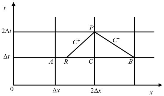
Figure 1.
Characteristic line method interpolation grid. Note(s): The horizontal coordinate Δx represents a unit length in meters (m), and the vertical coordinate Δt represents a time step in seconds (s). In the figure, A, B, C, and P denote points on the grid, R represents an interpolation point, and C+ and C− represent the two characteristic lines.
The pressure and flow rate parameters at point R in Figure 1 can be obtained by linear interpolation between points A and C. Consequently, simplifying Equation (6) yields the following system of equations:
The calculation formulas for the unknown parameters are as follows:
2.4.2. DGCM Model Solution Method
When using the DGCM model, both the time step and spatial discretization must satisfy the Courant–Lewy stability criterion. The maximum pressure in the transient flow can be estimated using the Rykov formula:
where represents the maximum pressure in the pipeline at the initial state (m), a0 is the wave speed of water (m/s), v0 is the flow velocity in the pipeline at the initial state (m/s), and g is the acceleration due to gravity (m/s2).
Substitute the maximum pressure obtained from Equation (8) into Equation (2) to find the maximum wave speed amax. Then, substitute amax into Equation (9) to determine the time step.
In the DGCM model, the gas cavity volume at the nodes changes continuously with the pipeline pressure. When liquid column separation occurs and Hi,j − Zi − HV < 0, calculations cannot be performed at this time. Therefore, a minimum pressure value hmin = 0.1 is defined. When Hi,j − Zi − HV < hmin, liquid column separation occurs in the pipeline. By simultaneously solving Equation (7) and the ideal gas law, the pressure and flow rate can be determined.
(1) When no liquid column separation occurs in the pipeline, that is, when Hi,j − Zi − HV > hmin, the solution is as follows:
The calculation formulas for the unknown parameters are as follows:
where Vi,j represents the gas cavity volume at node i at time j (m3), V0 is the volume between two adjacent nodes in the pipeline (m3), where V0 = A∆x, and φ is the weighting factor, taken as 1.0 in this study.
After computing using Equation (10), it is necessary to determine if liquid column separation has occurred. If Hi,j − Zi − HV > hmin, then the computed results are valid. If Hi,j − Zi − HV ≤ hmin, recalculation must be performed according to the liquid column separation model.
(2) When liquid column separation occurs in the pipeline, that is, when Hi,j − Zi − HV ≤ hmin, the solution is as follows:
After completing the calculation using Equation (11), it is necessary to check whether the gas cavity volume has recovered to the volume at the minimum pressure, where . If V − Vmin > 0, the computed results are valid. If V − Vmin ≤ 0, then Equation (10) needs to be recalculated.
2.5. Boundary Conditions
2.5.1. Leakage Boundary Conditions
Let be the upstream flow rate at the leakage hole, be the downstream flow rate at the leakage hole, and be the leakage flow rate at the hole. The external environment of the leakage hole is at atmospheric pressure. According to the principle of continuity of flow, the following relationship can be obtained:
Due to the occurrence of leakage, the compatibility characteristic Equation (6) can be rewritten as
Assuming the leakage flow at the leakage hole exits through the orifice, the leakage flow rate at the hole can be calculated using the following equation:
By solving Equations (12)–(14) simultaneously, the pressure HL at the leakage hole node and the upstream and downstream flow rates and of the leakage hole in the pipeline system can be determined.
2.5.2. Upstream Reservoir Boundary Conditions
The upstream boundary condition is a fixed water level, where the upstream head pressure remains constant, where H = H0. By combining the constant pressure H0 with the negative characteristic line equation C−, the reservoir flow rate at the upstream node can be determined.
2.5.3. Downstream Valve Boundary Conditions
The end of the water conveyance pipeline is equipped with a valve. The flow rate and pressure at this location are related to the valve’s opening and flow coefficient. The expression for calculating the flow rate QN at the valve is as follows:
where τ represents the relative opening of the valve, Qm is the flow rate when the valve is fully open under constant flow conditions, and Hm is the pressure when the valve is fully open under constant flow conditions. By combining Equation (17) with the positive characteristic line equation, the pressure at the downstream valve node can be obtained, as shown in Equation (18).
3. Result and Discussion
3.1. Subsection
The model constructed in this paper has the following basic operating conditions: The pipeline is at an elevation of 0 m and is horizontally positioned, without considering the effect of pipeline inclination α. The liquid in the pipeline is constant temperature tap water with a density of ρ = 1000 kg/m3, the upstream water level is constant at H0 = 15 m, the valve closes linearly over a time period of T = 3 s, the initial flow rate is Q0 = 0.03 m3/s, and the initial gas content rate is α0 = 0.01. The leakage location is XA = 500 m from the upstream water head, with an initial leakage amount of QL = 0.1, Q0 = 0.003. The valve starts closing at 100 s, the step length for unit pipeline length is dx = 10 m, and the time step length is dt = 0.02 s. The experimental system is illustrated in Figure 2, where 1 denotes the flow meter and 2 denotes the valve.
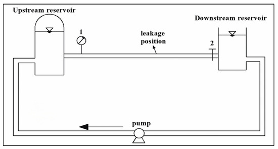
Figure 2.
Experimental setup diagram.
To validate the effectiveness and accuracy of the model and calculation program presented in this paper, the experimental data from Yipeng Zhang [30] was selected for comparison. Figure 3 shows the comparison between the measured and simulated results. In the initial stage, the measured and simulated results are quite consistent, with the error at the peak value being less than 5%. However, as time progresses, the error in the amplitude and phase of the transient flow increases. The possible reasons for this are as follows: the valve closure in the simulation is linear, which may differ from the valve closure method used in the experiment; there are discrepancies between the unsteady friction used in the simulation and the actual pipeline friction; and the DGCM model allows for variable wave speeds, leading to phase lags during the attenuation process. Although the numerical simulation in this paper shows a phase lag after 100.5 s, the simulated results are still highly consistent with the experimental results from the literature, validating the accuracy of the model constructed in this paper.
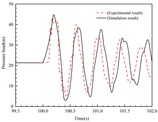
Figure 3.
Model verification.
3.2. Simulation Results and Analysis
3.2.1. The Impact of Valve Closing Time on End-of-Valve Pressure
Initial flow rate is Q0 = 0.03 m3/s, initial gas content rate is α0 = 0.01, leakage location distance from upstream head is XA = 500 m, and initial leakage amount is QL = 0.003 m3/s; keeping other basic conditions unchanged, change the valve closing time by setting it to T = 1 s, 2 s, 5 s, 10 s. The numerical simulation of the relationship between valve closing time and end-of-valve pressure is shown in Figure 4.
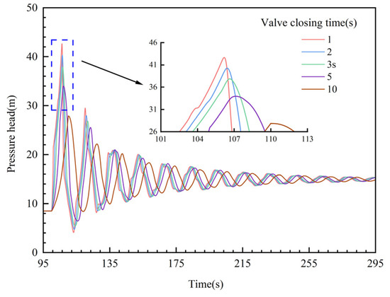
Figure 4.
Impact of valve closing time on end-of-valve pressure.
As shown in Figure 4, before the valve is closed, the end-of-valve pressure head remains at 8.63 m. As the valve closes, the end-of-valve pressure increases rapidly. However, this pressure rise occurs in two distinct phases: a pressure increase during the valve closing process and a pressure increase after the valve is fully closed. The mechanism of pressure increase is as follows: During the valve closing process, the inertia of the fluid causes it to continue flowing towards the valve, resulting in a temporary rise in pressure. After the valve is fully closed, the sustained increase in pressure is primarily due to fluid inertia and pressure wave effects. Additionally, the pressure waves generated by the valve closing propagate and reflect within the pipeline, causing further increases in pressure. These effects lead to a continued rise in pressure even after the valve is completely closed.
As the valve closing time increases, the time required to reach the peak pressure also increases. Under the five different conditions, the rate of pressure increase in the first phase slows down, while the time for the pressure to increase in the second phase decreases or even disappears, however, the rate of increase in this phase remains nearly consistent. When the valve closure time is 1 s, the pressure at the end continues to rise even as the valve is fully closed at 101 s, until the pressure head reaches its peak of 42.67 m at 106.2 s. When the valve closing time is increased to 10 s, the end-of-valve pressure head reaches its peak of 27.92 m at 110 s, the moment the valve is fully closed. This indicates that after extending the valve closing time for a certain period, the peak pressure occurs at the time when the valve is fully closed. It can also be inferred that the peak pressure time can be adjusted and controlled at this point. Extending the valve closing time aligns the peak pressure with the moment the valve is fully closed, which helps to smooth out pressure changes and reduce water hammer effects and pressure fluctuations. This means that in pipeline system design and operation, it is important to consider a longer valve closing time to decrease equipment pressure load, avoid instantaneous pressure shocks, and thereby improve the safety and reliability of the system.
3.2.2. The Impact of Initial Flow Rate on End-of-Valve Pressure
With an initial gas content rate of α0 = 0.01, a leakage location distance from the upstream head of XA = 500 m, an initial leakage amount of QL = 0.003 m3/s, and a valve closing time of T = 3 s, while keeping other initial conditions unchanged, the initial flow rate is varied. The initial flow rates are set to Q0 = 0.005 m3/s, 0.01 m3/s, 0.02 m3/s, 0.03 m3/s, and 0.04 m3/s. The numerical simulation of the relationship between different initial flow rates and the end-of-valve pressure is shown in Figure 5.
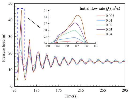
Figure 5.
Impact of initial flow rate on end-of-valve pressure.
As shown in Figure 5, before the valve is closed, the end-of-valve pressure remains constant. The initial flow rate is negatively correlated with the end-of-valve pressure. When the initial flow rate is 0.05 m3/s, the end-of-valve pressure is 14.8 m; whereas when the initial flow rate is 0.04 m3/s, the end-of-valve pressure is 3.9 m. A higher initial flow rate results in a lower end-of-valve pressure, which aligns with the well-known Bernoulli principle: For fluid flow at the same elevation, a higher flow velocity corresponds to lower pressure. After the valve is closed, a higher initial flow rate increases the rate of pressure rise in both the first and second phases under the five conditions, and the pressure peak is also delayed accordingly. When the initial flow rate is 0.005 m3/s, the pressure peak is 18.52 m; as the initial flow rate increases to 0.04 m3/s, the pressure peak rises to 45.92 m. An increase of 0.035 m3/s in flow rate results in a 147.95% increase in end-of-valve pressure. This indicates that, at valve closure, there is a significant positive correlation between the initial flow rate and the end-of-valve pressure. After the valve is closed, the initial increase in flow rate leading to a sharp rise in pressure indicates that even small changes in flow rate can significantly impact the pressure at the end of the valve. This sensitivity is particularly dangerous in systems with potentially large flow fluctuations, as it may cause the pipeline to rupture under the immense pressure, affecting the safe operation of the pipeline.
3.2.3. The Impact of Gas Content Rate on End-of-Valve Pressure
With an initial flow rate of Q0 = 0.03 m3/s, a leakage location distance from the upstream head of XA = 500 m, an initial leakage amount of QL = 0.003 m3/s, and a valve closing time of T = 3 s, while keeping other conditions constant, the gas content rate is varied. The initial gas content rates are set to α0 = 0.001, 0.005, and 0.01. The numerical simulation of the relationship between the gas content rate α₀ and the end-of-valve pressure is shown in Figure 6.
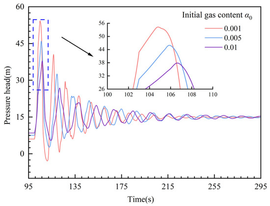
Figure 6.
The impact of gas content rate on end-of-valve pressure.
As shown in Figure 6, before the valve is closed, the water flow in the pipeline is stable. The end-of-valve pressure is positively correlated with the gas content rate; the higher the gas content rate in the pipeline, the greater the end-of-valve pressure. When the valve begins to gradually close, the time required for the end-of-valve pressure to reach its peak for the three conditions are 104.8 s, 105.9 s, and 106.6 s, respectively. This indicates that the gas content rate has a certain impact on the time required for the end-of-valve pressure to reach its peak. As the gas content rate increases, the rate of pressure-increase in the first phase of the three conditions remains largely unchanged, while the rate of pressure-increase in the second phase decreases. As the gas content rate in the pipeline increases, the amplitude of the end-of-valve pressure curve decreases. When the gas content rate is 0.001, the pressure peak is 54.27 m. As the gas content rate increases to 0.01, the pressure peak decreases to 37.89 m, representing a reduction of 30.18%. As the gas content rate increases, the time required for the pressure at the valve end to stabilize after the valve is closed also increases. This is because a higher gas content rate reduces the water hammer wave velocity, resulting in a longer time for the water hammer pressure wave to propagate over the same distance, thereby mitigating the impact on the pipeline. This characteristic can be considered in pipeline design to optimize gas content rate, thereby enhancing the system’s shock resistance, reducing the risk of pipeline damage, and improving overall safety and reliability.
3.2.4. The Impact of Leak Location on End-of-Valve Pressure
With an initial flow rate of Q0 = 0.03 m3/s, an initial gas content rate of α0 = 0.01, an initial leakage amount of QL = 0.003 m3/s, and a valve closing time of T = 3 s, while keeping other conditions constant, the leak location is varied. The leak locations are set to XA = 100 m, 300 m, 700 m, and 900 m. The numerical simulation of the relationship between different leak locations and the end-of-valve pressure is shown in Figure 7.
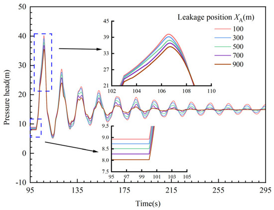
Figure 7.
The impact of leak location on end-of-valve pressure.
As shown in Figure 7, there is a negative correlation between the leakage location and the end-of-valve pressure both before and after valve closure. As the distance of the leakage location from the upstream reservoir increases, the end-of-valve pressure during stable flow before valve closure, as well as the pressure peak after valve closure, decreases. As the distance of the leakage location from the upstream reservoir increases, the pressure-increase patterns in the first and second phases remain largely consistent across the five scenarios. While the leakage location does affect the magnitude of the end-of-valve pressure, it does not influence the time at which the pressure peak is reached.
3.2.5. The Impact of Leakage Amount on End-of-Valve Pressure
With an initial flow rate of Q0 = 0.03 m3/s, an initial gas content rate of α0 = 0.01, a leakage location at XA = 500 m from the upstream head, and a valve closure time of T = 3 s, and keeping other conditions unchanged, the leakage amount is varied to QL = 0.01Q0, 0.1Q0, 0.2Q0, and 0.3Q0. The numerical simulation of the relationship between different leakage amounts and the pressure at the end of the valve is shown in Figure 8.
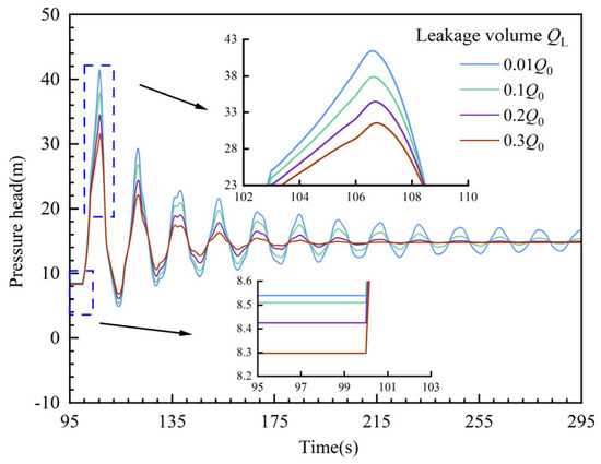
Figure 8.
The impact of leakage amount on end-of-valve pressure.
As shown in Figure 8, before the valve closure, different leakage amounts have little impact on the pressure at the end of the valve, with the maximum pressure difference among the four conditions being only 0.24 m. As the valve closes, the pressure at the end of the valve increases sharply, and the leakage amount is negatively correlated with the pressure at the end of the valve. As the leakage amount increases, the pressure-increase trends in the first and second sections under the four conditions are generally similar. With increasing leakage amount, the peak pressure at the end of the valve decreases. When the leakage amount is 0.01Q0, the peak pressure is 41.84 m; when the leakage amount increases to 0.3Q0, the peak pressure decreases to 31.57 m, representing a reduction of 24.55%. The variation in leakage amount will affect the pressure magnitude at the valve outlet but will not affect the time at which the pressure peak at the valve outlet is reached.
4. Prediction of Leakage Location
4.1. Data Preprocessing
This paper develops a leakage location prediction model for water supply pipelines based on a backpropagation (BP) neural network and employs a genetic algorithm to optimize the prediction accuracy of the model. Firstly, the creation of the dataset and the preprocessing of the data are conducted. The study selects four parameters from the numerical simulation variables—valve closing time, initial flow rate, gas content, and leakage amount—as input feature vectors. To eliminate the dimensional differences among the aforementioned parameters, normalization of the data is performed before training the neural network. This normalization process helps to improve the model’s performance and training stability. In this paper, all sample values in the dataset are within the [0, 1] interval. The transformation formula is as follows:
where represents the normalized input value and Xi denotes the original input sample data. Xmax is the maximum value of the original data and Xmin is the minimum value of the original data.
The experimental data used in constructing the neural network model comprises 262 samples. During the data preprocessing stage, the dataset is divided into a training set of 227 samples and a validation set of 35 samples. Firstly, the training set is used to fit the data samples and generate the training model. During this process, the validation set is employed to assess the model’s performance, and model parameters are adjusted based on the results obtained from the training set. Thus, by leveraging the neural network’s powerful learning capabilities and function approximation abilities, a mapping relationship between the leakage location and the various influencing factors can be established.
4.2. Neural Network Model
The backpropagation (BP) neural network is a type of artificial neural network that updates weights through error feedback. The BP neural network model consists of three components: the input layer, the hidden layer, and the output layer. It possesses non-linear mapping capabilities and good self-learning abilities; however, it is prone to becoming trapped in local optima and may have limitations in fitting complex non-linear systems. Therefore, it is necessary to optimize the BP neural network. This paper employs the genetic algorithm (GA) to simulate the natural evolution process in order to seek an optimal solution for improving the BP neural network. The topology of the BP neural network model is shown in Figure 9. The number of nodes in the input layer is 4, and the number of nodes in the output layer is 1, corresponding to the number of features for the input and output variables, respectively. The number of nodes in the hidden layer is estimated using the following empirical formula:
where M represents the number of neurons in the hidden layer of the BP network. m and n represent the number of nodes in the input and output layers. a is a constant within the range [0, 10].
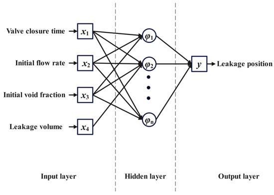
Figure 9.
Neural network architectures.
The genetic algorithm-backpropagation neural network (GA-BP neural network) utilizes a genetic algorithm to optimize the weights and thresholds of the neural network. The fitness of each individual is calculated, with individuals having low fitness being eliminated and those with high fitness being retained. The new population inherits information from the previous generation and is superior to it. This process is repeated iteratively to find the optimal solution. The GA-BP genetic algorithm encodes the initial weights and thresholds, and then employs mechanisms such as selection, crossover, and mutation to ultimately obtain an approximate solution. This optimal solution is then used to replace the initial weights and thresholds in the BP neural network, followed by training the optimized network. In this study, a population size of 40 is selected, with a crossover probability of 0.6 and a mutation probability of 0.05. The algorithm terminates when the fitness of the optimal individual no longer decreases or when the maximum number of iterations is reached. The flowchart of the GA-BP algorithm is shown in Figure 10:
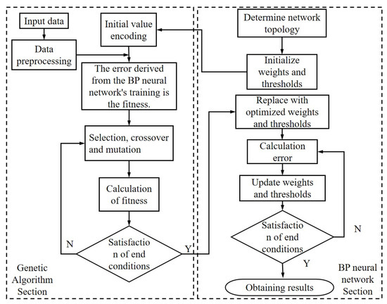
Figure 10.
GA-BP algorithm procedure.
The specific training operations of the GA-BP neural network are as follows:
- Population Initialization. Before solving the problem, parameters need to be encoded to form the initial solutions of the population. Real-number encoding is used to connect the weights and thresholds between the layers. Each individual is represented as a real number string, consisting of four parts: the weights connecting the input layer and hidden layer, the thresholds of the hidden layer, the weights connecting the hidden layer and output layer, and the thresholds of the output layer. The length of the encoding is calculated using the following formula:where l represents the encoding length. m is the number of nodes in the input layer of the BP neural network. sl is the number of neurons in the hidden layer. n is the number of nodes in the output layer.
- Fitness Function. The fitness function measures the quality of the individuals in the population by summing the absolute errors between the actual outputs and the desired outputs of the neural network. In this study, it refers to the difference between the true leakage location and the predicted value. A smaller error indicates a better fitness of the individual. The formula for the fitness function is as follows:where F represents the fitness value. n is the number of training samples. yi and represent the actual value and predicted value of the i-th node in the BP neural network.
- Selection Operation. The purpose of the selection operation is to increase the probability of selecting individuals with smaller errors. Since the fitness function indicates that a smaller fitness value corresponds to a smaller error, the reciprocal of the fitness value is used. The formula is as follows:where represents the fitness value of the i-th individual. k is a coefficient. is the probability of the individual being selected. n is the number of individuals in the population.
- Crossover Operation. The crossover operation involves performing position-based crossover between different chromosomes to achieve gene exchange, thereby forming new individuals. Since the individuals are encoded using real numbers, real-number crossover methods are used. The crossover operation between the -th chromosome and the -th chromosome at the -th position is performed as follows:where b is a random number within the interval [0, 1].
- Mutation Operation. Select the -th individual’s -th gene for mutation. The operation method is as follows:where amax and amin represent the upper and lower bounds of the gene aij. g is the current iteration number. Gmax is the maximum number of evolutionary iterations. r is a random number within the interval [0, 1] and r2 is another random number.
4.3. Leakage Location Prediction
Table 1 compares the performance of different numbers of neurons in the hidden layer. It can be concluded that with 10 neurons, both the correlation coefficient and the error are relatively optimal. Therefore, the number of neurons in the hidden layer is chosen to be 10.

Table 1.
Performance comparison of neuron numbers in different hidden layers.
Figure 11a,b presents the prediction results of the test set for the BP neural network and the GA-BP neural network, respectively. In this study, 227 samples were used for training and 35 samples for prediction. To prevent overfitting, the data for the test set and training set were randomly selected. The results indicate that the GA-BP neural network model performs better.
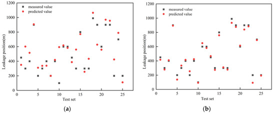
Figure 11.
Predict results. (a) BP neural network predicted results. (b) GA-BP neural network predicted results.
To investigate the discrepancy between the predicted and measured values of the GA-BP neural network model, this study predicted experimental data using the trained model. The prediction error of the GA-BP neural network model is shown in Figure 12a. The results indicate a mean absolute percentage error (MAPE) of 9.26%, demonstrating good prediction performance with errors concentrated within the 10% range. To further validate the model’s accuracy and generalization ability, an additional 16 simulation conditions were tested, as shown in Figure 12b. The results revealed a MAPE of 10.13%, indicating satisfactory prediction performance. This indicates that neural networks can predict pipeline leakage locations with a relatively high degree of accuracy.
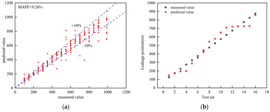
Figure 12.
Error between experimental and predicted values. (a) Error between experimental and predicted values. (b) Comparison of predicted results with experimental results.
5. Conclusions
This paper establishes a transient flow model of water pipeline leakage considering the effects of unsteady friction, analyzes the impact of different factors on the end-of-valve pressure, and uses a neural network model to predict the leakage location of the pipeline. The main conclusions are as follows:
- (1)
- Valve closing time has a significant impact on the end-of-valve pressure. When the valve closing time is increased from 1 s to 10 s, the pressure peak decreases from 42.67 m to 27.92 m, a reduction of 34.57%. Increasing the valve closing time also delays the arrival time of the pressure peak at the valve end.
- (2)
- Initial flow rate, leakage amount, and gas content rate have a certain impact on the end-of-valve pressure. After valve closure, the larger the initial flow rate, the lower the gas content rate, and the smaller the leakage amount, the greater the pressure peak at the valve end. When the initial flow rate increases from 0.005 m3/s to 0.04 m3/s, the pressure peak rises from 18.52 m to 45.92 m, an increase of 147.95%. When the gas content rate increases from 0.001 to 0.01, the pressure peak decreases from 54.27 m to 37.89 m, a reduction of 30.18%. As the leakage rate increases from 0.01Q₀ to 0.3Q₀, the pressure peak decreases from 41.81 m to 31.57 m, a decrease of 24.55%.
- (3)
- The GA-BP neural network can accurately predict the leakage location. The prediction model constructed using the GA-BP neural network had a mean absolute percentage error (MAPE) of 7.72% when predicting experimental data, indicating good prediction performance. The GA-BP neural network model can effectively solve complex prediction problems influenced by multiple factors, providing a new feasible approach for predicting pipeline leakage locations.
Author Contributions
Conceptualization, Q.Z., Z.Z., B.H., Z.Y. (Ziyuan Yu), X.L. and Z.Y. (Zhendong Yang); Data curation, B.H.; Formal analysis, Z.Z.; Investigation, Z.Z.; Methodology, Q.Z., Z.Z., B.H. and Z.Y. (Zhendong Yang); Project administration, Q.Z.; Software, Z.Z. and B.H.; Supervision, Q.Z. and Z.Y. (Ziyuan Yu); Validation, Z.Z.; Writing—original draft, Z.Z.; Writing—review and editing, Q.Z. All authors have read and agreed to the published version of the manuscript.
Funding
This work is financially supported by the General Program of National Natural Science Foundation of China (No. 52376149), and the Key Scientific Research Program Funded by Shaanxi Provincial Education Department (No. 20JY044).
Data Availability Statement
Data is contained within the article.
Conflicts of Interest
Author Ziyuan Yu was employed by the Qingdao Warbus Intelligent Experiment Technology Co., Ltd. The remaining authors declare that the research was conducted in the absence of any commercial or financial relationships that could be construed as a potential conflict of interest.
References
- Cao, H.; Nistor, I.; Mohareb, M. Effect of Boundary on Water Hammer Wave Attenuation and Shape. J. Hydraul. Eng. 2020, 146, 4020001. [Google Scholar] [CrossRef]
- Kim, S.; Lee, K.; Kim, K. Water hammer in the pump-rising pipeline system with an air chamber. J. Hydrodyn. Ser. B 2015, 26, 960–964. [Google Scholar] [CrossRef]
- Bergant, A.; Simpson, A.R.; Tijsseling, A.S. Water hammer with column separation: A historical review. J. Fluids Struct. 2006, 22, 135–171. [Google Scholar] [CrossRef]
- Bergant, A.; Tusseling, A.S.; Vitkovsky, J.P.; Covas, D.I.C.; Simpson, A.R.; Lambert, M.F. Parameters affecting water-hammer wave attenuation, shape and timing Part 1: Mathematical tools. J. Hydraul. Res. 2008, 46, 373–381. [Google Scholar] [CrossRef]
- Bergant, A.; Tijsseling, A.S.; Vitkovsy, J.P.; Covas, D.I.C.; Simpson, A.R.; Lambert, M.F. Parameters affecting water-hammer wave attenuation, shape and timing Part 2: Case studies. J. Hydraul. Res. 2008, 46, 382–391. [Google Scholar] [CrossRef]
- Wang, C.; Yang, J.; Nilsson, H. Simulation of Water Level Fluctuations in a Hydraulic System Using a Coupled Liquid-Gas Model. Water 2015, 7, 4446–4476. [Google Scholar] [CrossRef]
- Duan, H.; Ghidaoui, M.; Lee, P.J.; Tung, Y. Unsteady friction and visco-elasticity in pipe fluid transients. J. Hydraul. Res. 2010, 48, 354–362. [Google Scholar] [CrossRef]
- Zhou, L.; Wang, H.; Liu, D.; Ma, J.; Wang, P.; Xia, L. A second-order Finite Volume Method for pipe flow with water column separation. J. Hydro-Environ. Res. 2017, 17, 47–55. [Google Scholar] [CrossRef]
- Adamkowski, A.; Lewandowski, M. Investigation of Hydraulic Transients in a Pipeline with Column Separation. J. Hydraul. Eng. 2012, 138, 935–944. [Google Scholar] [CrossRef]
- Adamkowski, A.; Lewandowski, M. Consideration of the Cavitation Characteristics of Shut-off Valves in Numerical Modelling of Hydraulic Transients in Pipelines with Column Separation. Procedia Eng. 2014, 70, 1027–1036. [Google Scholar] [CrossRef][Green Version]
- Jiang, D.; Li, S.; Edge, K.A.; Zeng, W. Modeling and simulation of low pressure oil-hydraulic pipeline transients. Comput. Fluids 2012, 67, 79–86. [Google Scholar] [CrossRef]
- Warda, H.A.; Wahba, E.M.; El-Din, M.S. Computational Fluid Dynamics (CFD) simulation of liquid column separation in pipe transients. Alex. Eng. J. 2020, 59, 3451–3462. [Google Scholar] [CrossRef]
- Mehmood, K.; Zhang, B.; Jalal, F.E.; Wan, W. Transient flow analysis for pumping system comprising pressure vessel using unsteady friction model. Int. J. Mech. Sci. 2023, 244, 108093. [Google Scholar] [CrossRef]
- Daude, F.; Galon, P.; Douillet-Grellier, T. 1D/3D Finite-Volume coupling in conjunction with beam/shell elements coupling for fast transients in pipelines with fluid–structure interaction. J. Fluids Struct. 2021, 101, 103219. [Google Scholar] [CrossRef]
- Srinivasan, S.; O’Malley, D.; Hyman, J.D.; Karra, S.; Viswanathan, H.S.; Srinivasan, G. Transient flow modeling in fractured media using graphs. Phys. Rev. E 2020, 102, 052310. [Google Scholar] [CrossRef]
- Pan, B.; Keramat, A.; Duan, H. Energy Analysis for Transient-Leak Interaction and Implication to Leak Detection in Water Pipeline Systems. J. Hydraul. Eng. 2023, 149, 04023031. [Google Scholar] [CrossRef]
- Mosaheb, M.; Zeidouni, M. Pressure Transient Analysis to Determine Anisotropic Fault Leakage Characteristics. J. Hydrol. Eng. 2020, 25, 04020046. [Google Scholar] [CrossRef]
- Fathi-Moghadam, M.; Kiani, S. Simulation of transient flow in viscoelastic pipe networks. J. Hydraul. Res. 2020, 58, 531–540. [Google Scholar] [CrossRef]
- Keramat, A.; Tijsseling, A.S.; Hou, Q.; Ahmadi, A. Fluid-structure interaction with pipe-wall viscoelasticity during water hammer. J. Fluids Struct. 2012, 28, 434–455. [Google Scholar] [CrossRef]
- Zhu, Y. Study on Steady-State Vibration and Transient Process in Water Conveyance Pipeline Based on Gas-Liquid Two-Phase Flow. Ph.D. Thesis, Harbin Institute of Technology, Harbin, China, 2018; p. 154. [Google Scholar]
- Medeiros, V.d.S.; dos Santos, M.D.; Brito, A.V. Case Study for Predicting Failures in Water Supply Networks Using Neural Networks. Water 2024, 16, 1455. [Google Scholar] [CrossRef]
- Gorenstein, A.; Kalech, M.; Hanusch, D.F.; Hassid, S. Pipe fault prediction for water transmission mains. Water 2020, 12, 2861. [Google Scholar] [CrossRef]
- Feng, G.; Zhang, K.; Wan, H.; Yao, W.; Zuo, Y.; Lin, J.; Liu, P.; Zhang, L.; Yang, Y.; Yao, J.; et al. Enhancing Oil–Water Flow Prediction in Heterogeneous Porous Media Using Machine Learning. Water 2024, 16, 1411. [Google Scholar] [CrossRef]
- Ye, J.; Do, N.C.; Zeng, W.; Lambert, M. Physics-informed neural networks for hydraulic transient analysis in pipeline systems. Water Res. 2022, 221, 118828. [Google Scholar] [CrossRef]
- Wang, W.; Sun, H.; Guo, J.; Lao, L.; Wu, S.; Zhang, J. Experimental study on water pipeline leak using In-Pipe acoustic signal analysis and artificial neural network prediction. Measurement 2021, 186, 110094. [Google Scholar] [CrossRef]
- Ribeiro, A.M.; Grossi, C.D.; Santos, B.F.; Santos, R.B.; Fileti, A.M.F. Leak Detection Modeling of a Pipeline Using Echo State Neural Networks. Comput. Aided Chem. Eng. 2018, 43, 1231–1236. [Google Scholar]
- Pérez-Pérez, E.J.; López-Estrada, F.R.; Valencia-Palomo, G.; Torres, L.; Puig, V.; Mina-Antonio, J.D. Leak diagnosis in pipelines using a combined artificial neural network approach. Control. Eng. Pract. 2021, 107, 104677. [Google Scholar] [CrossRef]
- Bohorquez, J.; Lambert, M.F.; Alexander, B.; Simpson, A.R.; Abbott, D. Stochastic Resonance Enhancement for Leak Detection in Pipelines Using Fluid Transients and Convolutional Neural Networks. J. Water Resour. Plan. Manag. 2022, 148, 04022001. [Google Scholar] [CrossRef]
- Liu, Z.; Yang, X.; Wu, M.; Mu, W.; Liu, G. Leveraging deep learning techniques for ship pipeline valve leak monitoring. Ocean. Eng. 2023, 288, 116167. [Google Scholar]
- Zhang, Y. Numerical Simulation and Experimental Research on Transient Characteristic and Leak Detection of Pressurized Pipeline. Ph.D. Thesis, Wuhan University, Wuhan, China, 2018; p. 144. [Google Scholar]


Disclaimer/Publisher’s Note: The statements, opinions and data contained in all publications are solely those of the individual author(s) and contributor(s) and not of MDPI and/or the editor(s). MDPI and/or the editor(s) disclaim responsibility for any injury to people or property resulting from any ideas, methods, instructions or products referred to in the content. |
© 2024 by the authors. Licensee MDPI, Basel, Switzerland. This article is an open access article distributed under the terms and conditions of the Creative Commons Attribution (CC BY) license (https://creativecommons.org/licenses/by/4.0/).