Abstract
Wastewater remaining in pipes for extended periods can create anaerobic environments, fostering the growth of anaerobic bacteria and producing harmful gases such as methane and hydrogen sulfide. Additionally, certain structures within drainage systems, such as drop shafts and vertical shafts, induce turbulent flow, causing the release of dissolved harmful gases, which pose significant risks to public health and urban infrastructure. This study focused on the investigation and analysis of vertical shafts with helical tray structures in drainage systems. Using ANSYS 2021 R2 software, simulations of the shafts were conducted by employing the standard k-ε turbulence model and Eulerian multiphase flow method to simulate the shaft’s operation and obtain various parameters of hydrogen sulfide release. Concurrently, a scale model constructed in the laboratory was used to study and analyze the release of hydrogen sulfide gas dissolved in water from this type of structure. Combining the simulation and laboratory experiments, the hydrogen sulfide gas release rate from water in this structure was 0.05–0.4%. This research provides a reference for the study and control of hydrogen sulfide gas release.
1. Introduction
Urban drainage systems are crucial infrastructure for modern cities and industrial enterprises, essential for maintaining the normal functioning of urban life, protecting the environment from pollution, and ensuring public health and quality of life [1]. These systems encompass multiple aspects including the collection, transportation, treatment, utilization, and final discharge of wastewater, forming a complex and efficient processing network [2]. With the accelerated urbanization process and continuous population growth, the scale of urban wastewater drainage systems has expanded, leading to longer pipelines. Prolonged retention of wastewater in these pipes creates anaerobic environments, fostering the growth of anaerobic microorganisms [3,4]. These anaerobic bacteria produce harmful gases such as methane and hydrogen sulfide. Methane, a colorless, odorless, and flammable gas, can cause explosions when its concentration in the air reaches a certain level [5]. Hydrogen sulfide, a highly toxic gas, strongly irritates the respiratory system and mucous membranes [6,7]. The continuous release of these gases not only poses a threat to human health, but also risks causing corrosion and explosions in urban sewage pipelines, severely endangering the safe operation of cities and social stability [8,9].
In urban drainage system design, topography and pipeline length are crucial factors determining the layout and functionality of drainage networks. Especially in areas with complex terrain or large urban expanses, drainage pipelines often need to overcome significant elevation differences to ensure the smooth flow of wastewater [10,11]. In order to effectively connect pipelines at different heights, engineers have designed special structures such as ordinary drop wells and deeper vertical shafts to ensure the efficiency and safe operation of the system [12]. Drop structures are used to control the flow rate and direction of wastewater, allowing it to safely fall from higher to lower pipes. Without drop shafts, direct flow from high to low areas could result in excessively high flow speeds, increasing the pipe wear and potentially causing pipe damage or overflow accidents due to the high impact force [13,14]. Inside drop shafts, structures like buffer platforms or energy dissipation devices are often designed to mitigate the impact of water flow, thus dispersing energy and reducing physical stress on the pipes [15]. Vertical shafts are another critical facility connecting horizontal sewage pipes to vertical (or inclined) drainage structures, facilitating vertical or inclined wastewater transport within the system [16]. Adding special structures inside vertical shafts can achieve similar energy dissipation effects as drop shafts. However, due to the significant elevation differences in these systems, such structures can cause turbulent flow, leading to the release of dissolved harmful gases and posing greater risks [17,18].
Therefore, to ensure the safe and effective operation of urban drainage systems, it is essential to study the concentration of harmful gases and their release rates in various structures within the drainage system. Additionally, necessary cleaning and flushing should be conducted to eliminate potential safety hazards.
2. Mathematical and Experimental Models
2.1. Simulation Experiment Mathematical Model
2.1.1. Calculation Area and Mesh Division
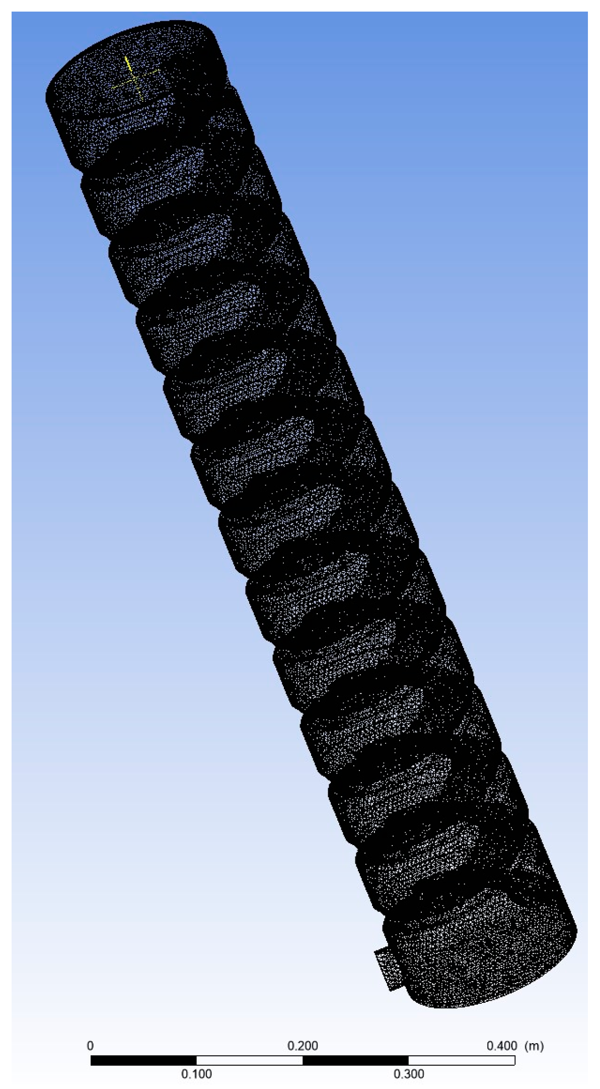
Based on a 1:60 scale, a simulation model was created using SolidWorks in combination with SpaceClaim 2021 R2 software. The model parameters are shown in Table 1, and the final model is illustrated in Figure 1. Using Fluent 2021 R2 software, an unstructured mesh was applied to the computational domain, as depicted in Figure 2.

Table 1.
Simulation experimental model parameters.
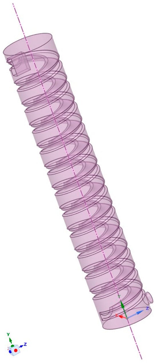
Figure 1.
Simulation experimental model.
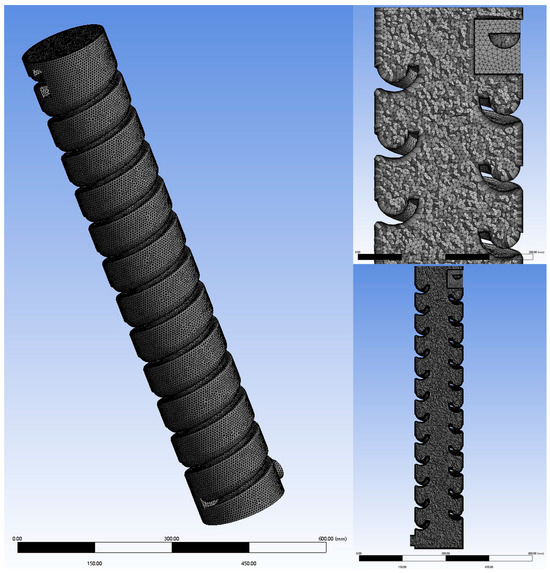
Figure 2.
Model meshing.
2.1.2. Boundary Conditions
The inlet boundary condition was defined as a velocity inlet, using water as the solvent. The volume fractions of water and hydrogen sulfide were calculated using Equation (1), resulting in 0.993 and 0.007 for a hydrogen sulfide solution of 10 mg/L, 0.985, and 0.015 for 20 mg/L, and 0.971, and 0.029 for 40 mg/L, respectively. Water flowed through an open inlet into the vertical shaft, subsequently descending along the helical tray inside the shaft. The outlet boundary condition was set as a pressure outlet; when the water level is high, the flow in the shaft is under pressure. To reasonably simulate the outlet flow, the outlet pressure was taken as the average of the measured maximum and minimum pressures [19,20].
The hydrogen sulfide volume fraction calculation formula is as follows:
In the formula, represents the volume fraction of hydrogen sulfide; is the mass of hydrogen sulfide dissolved in water; is the density of hydrogen sulfide with a value of ; is the density of the solvent water with a value of ; and is the total volume of the solution.
The wall boundary condition was set as a no-slip boundary. In viscous flow, the wall is assumed to be a no-slip boundary condition by default, with the viscous sublayer treated using the wall function method. The algorithm employed the finite volume method with implicit scheme iteration, and the velocity–pressure coupling was handled using the phase coupled SIMPLE algorithm [21,22].
2.1.3. Standard k-ε Turbulence Model
The k-ε turbulence model was employed for the complex curved free surface and boundary conditions, using unstructured meshes to discretize the three-dimensional computational domain. The Eulerian method, suitable for multiphase flow, was introduced for the solution [23]. The k-ε model assumes isotropy for each component of the Reynolds stress and uses the Eulerian method to calculate, which aligns well with the actual situation. The continuity equation, momentum equation, and k-ε equations of the standard k-ε turbulence model are as follows [24,25].
Continuity equation:
Momentum equation:
equation:
equation:
In the formula, is time; and are the velocity and coordinate components, respectively; and are the density and molecular viscosity coefficients, respectively; is the modified pressure; is the turbulent viscosity coefficient, which can be derived from the turbulent kinetic energy and the turbulent dissipation rate ; and . is an empirical constant, ; and are the turbulent Prandtl numbers for and , respectively, , ; and are equation constants , , respectively; and is the term representing the generation of turbulent kinetic energy due to the mean velocity gradients, specifically:
2.1.4. Mass Transport and Component Diffusion Equations
Mass and component transport occur between water and hydrogen sulfide.
The mass transport equation is [26]:
In the equation, and represent the turbulent fluctuations of the velocity and liquid phase mass fraction. The right side of the equation is the diffusion source term caused by turbulence, which is closed using Fick’s law.
In the equation, is the turbulent dynamic viscosity and is the Schmidt number.
Component diffusion equation [27]:
The component transport equation estimates the mass fraction of each substance through the convection–diffusion equation of the th substance. The general form of the component transport equation is:
In the equation, is the mass fraction of the th component; is the kinematic viscosity of the gas; is the net production rate of the th component due to chemical reactions; is the diffusion flux of the th component; and represents the additional production rate of the th component caused by discrete phases and user-defined source terms.
2.2. Experimental Model
2.2.1. Experimental Model Parameters
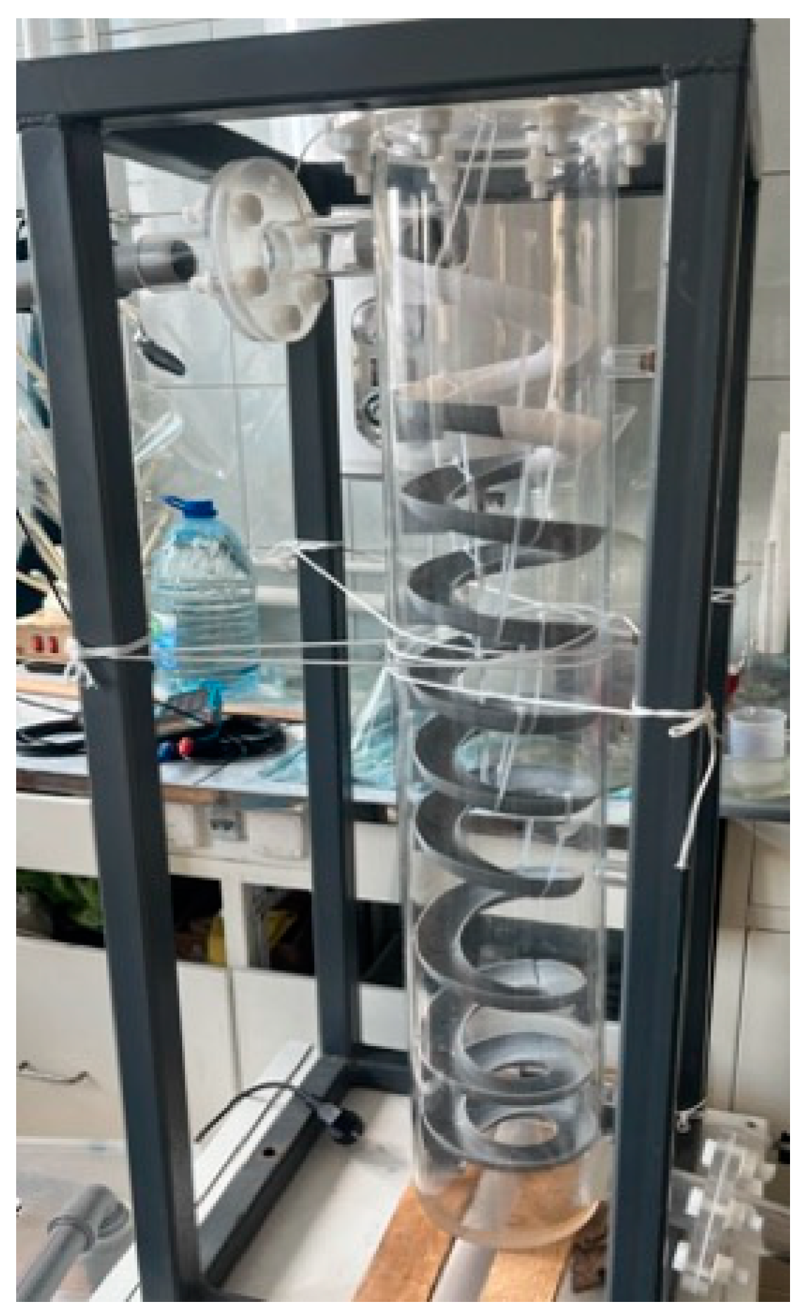
This experimental model was based on an engineering project in the northern part of Saint Petersburg, created at a 1:60 scale. The model is shown in Figure 3. The vertical shaft of the model was made of acrylic, which offers corrosion resistance and high transparency [28], ensuring the safety and effectiveness of the experiment. The helical tray structure inside the shaft was produced using 3D printing technology, which allows for the convenient design and manufacturing of the required components [29]. This structure was printed and installed inside the vertical shaft. The parameters of the vertical shaft model and the internal helical tray are presented in Table 2.

Figure 3.
Experimental shaft model.
Table 2.
Experimental model parameters.
2.2.2. Experimental Water Parameters
Due to the difficulty in obtaining actual wastewater and the significant variability among different wastewater samples, sodium sulfide nonahydrate was used to prepare the experimental water. Its dissolution in water is described by the following chemical equation:
The experimental sulfide ion A concentrations were set at 10 mg/L, 20 mg/L, and 40 mg/L. Given the low concentration settings, a 5 g/L sodium sulfide nonahydrate solution was prepared first. Then, a specific amount of this prepared solution was added to a reagent bottle containing 5 L of pure water to achieve the desired concentrations [30]. The solution preparation table, derived from the following equation, is shown in Table 3.
Table 3.
Solution preparation table.
In the equation, is the required mass of sodium sulfide nonahydrate; is the required mass of sulfide ions; is the molar mass of sodium sulfide nonahydrate with a value of ; and is the molar mass of sulfur with a value of .
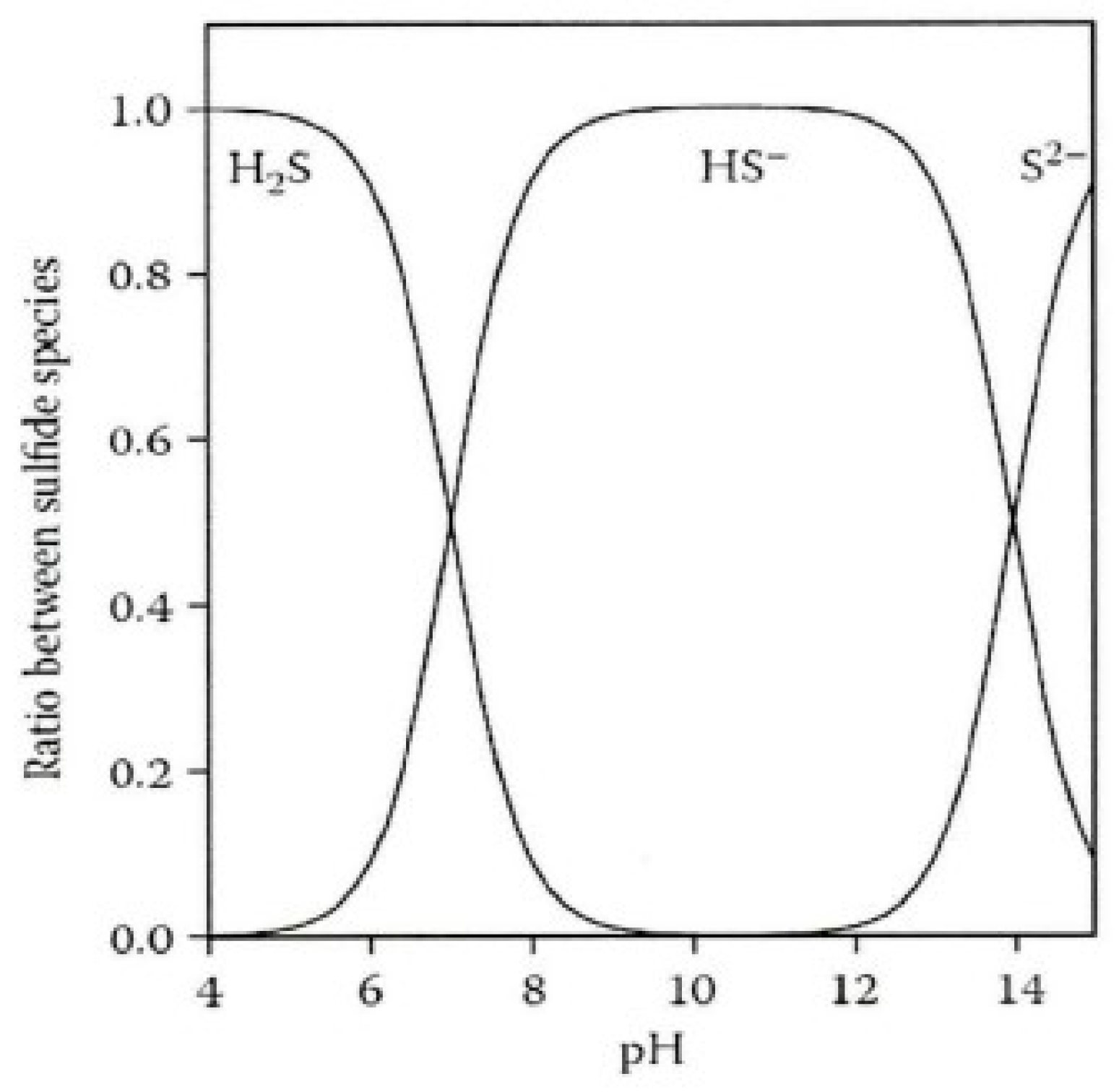
Given the varying conversion rates of hydrogen sulfide at different pH levels (see Figure 4), this experiment used an experimental water environment with a pH of 5 [31]. The equation for its degassing release from water is:
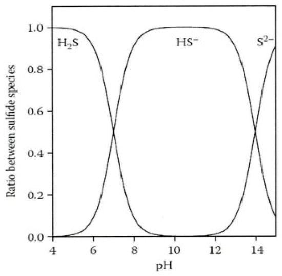
Figure 4.
Morphological transformation of sulfides under different pH environments.
The degassing rate of hydrogen sulfide gas should be:
where is the degassing rate; represents the hydrogen sulfide concentration data measured by the gas detector; denotes the volume of hydrogen sulfide gas released into the gas detector; is the concentration of hydrogen sulfide in the solution; and is the volume of the aqueous solution.
2.2.3. Experimental Circulation System
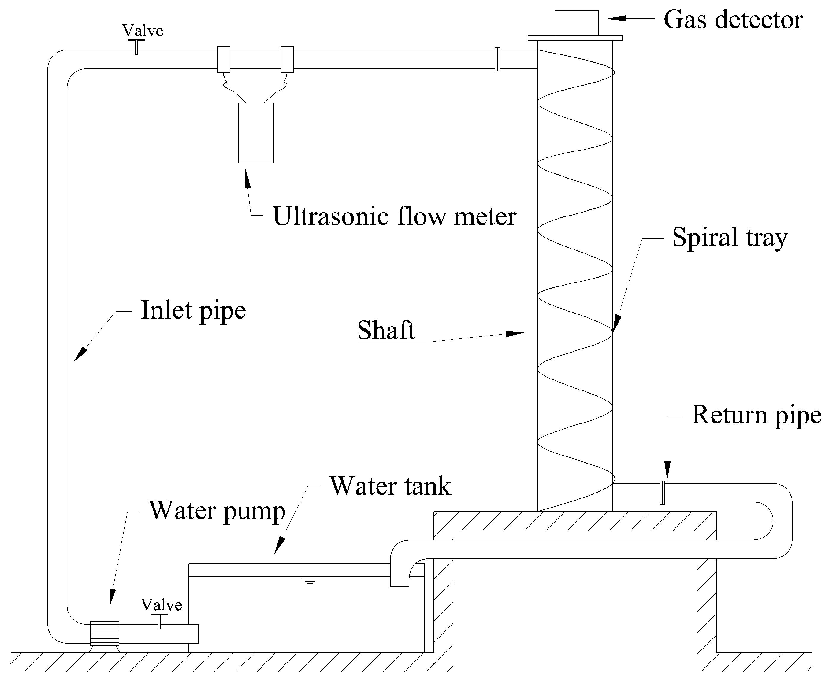
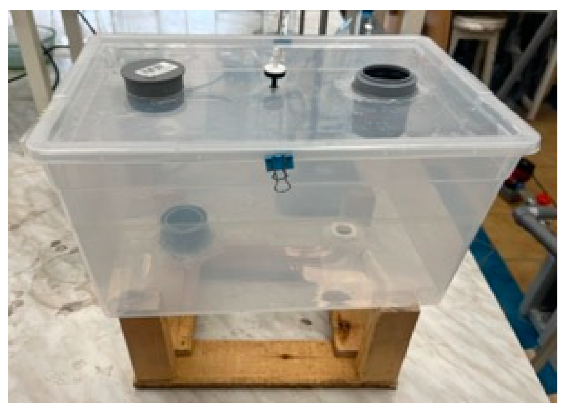
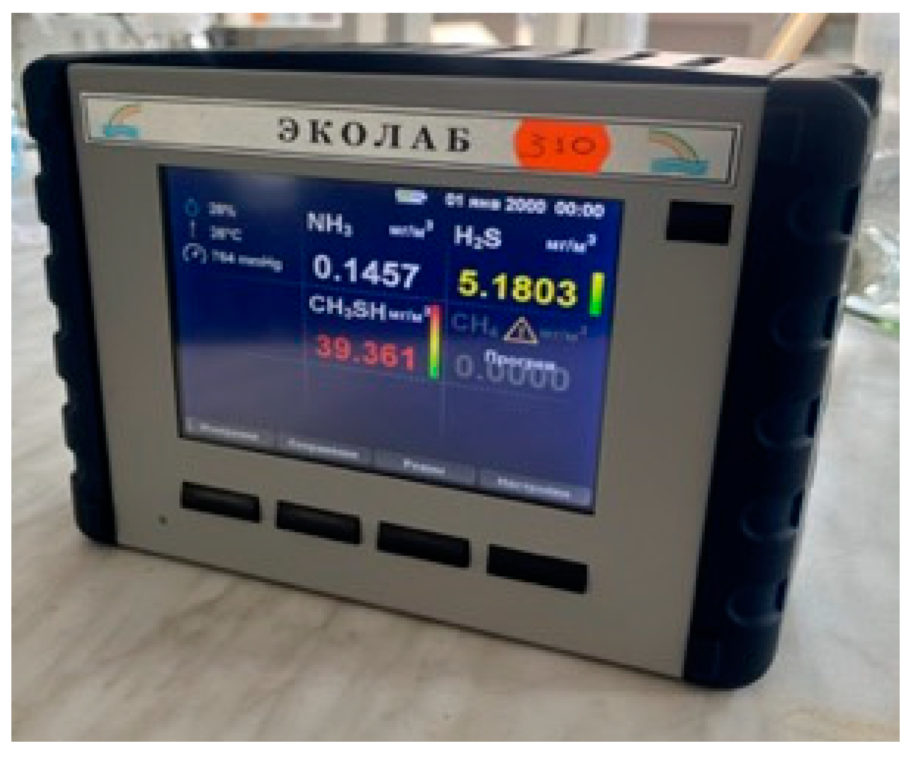
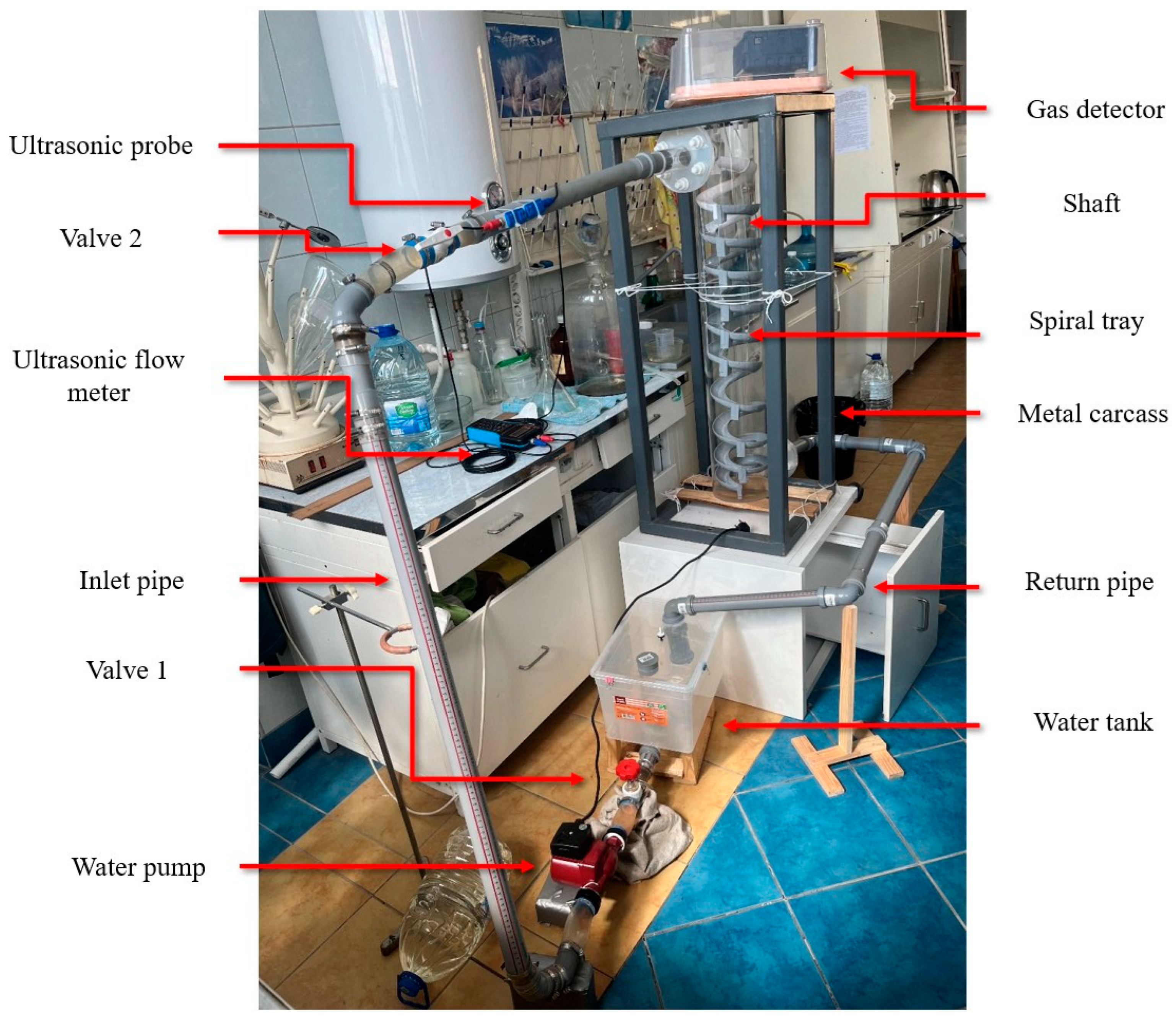
For experimental convenience, a water circulation system was constructed for this experiment, as shown in Figure 5. Since this system was to be used continuously in subsequent research, a water tank for the circulation system was created under limited conditions. The tank consisted of an experimental water inlet, an air inlet, a circulation water outlet, a circulation water inlet, and a drain outlet. The tank lid was sealed tightly, with rubber gaskets added around the lid and secured with clips to enhance the tank’s airtightness. The experimental water tank is shown in Figure 6. The tank was connected to valves and water supplies, with an ultrasonic flowmeter installed on the inlet pipe to measure the water flow rate and velocity entering the vertical shaft. A valve before the flowmeter was used to adjust the flow rate. Finally, the experimental water flowed back into the circulation tank through the drainage pipe. A hydrogen sulfide gas detector was placed at the top of the vertical shaft (the gas detector is shown in Figure 7) to record the concentration of hydrogen sulfide gas released. The gas detector employed solid-state metal oxide semiconductor sensing technology, utilizing a sensor composed of two thin films—one as a heating element and the other as a hydrogen sulfide-sensitive gas sensor. Both films were vacuum-deposited on a silicon chip. The heating element increased the operating temperature of the gas sensor to a level where it could react with the hydrogen sulfide gas. The metal oxide on the gas sensor dynamically displayed changes in the hydrogen sulfide concentration with high sensitivity, ranging from parts per billion to percent levels. This technology ensures that the detector will remain stable and durable in most industrial environments for over a decade. The circulation system is shown in Figure 8.
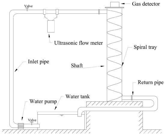
Figure 5.
Experimental system diagram.

Figure 6.
Experimental water tank.

Figure 7.
Gas detector.

Figure 8.
Experimental circulation system.
3. Research and Analysis of Results
3.1. Analysis of Gas Flow within the Shaft
As water flowed through the helical tray, the turbulent current released hydrogen sulfide gas dissolved in the water. Simultaneously, the water flow agitated the air, as shown in Figure 9. The entrainment of air caused the released hydrogen sulfide gas to move upward and reach the top. The entrainment phenomenon observed during the operation of the vertical shaft aligned with its actual operating conditions.
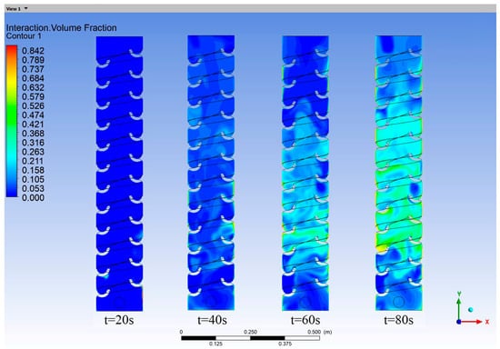
Figure 9.
Hydrogen sulfide gas volume fraction contour map in the vertical shaft at different times.
3.2. Simulation Analysis of Hydrogen Sulfide Release
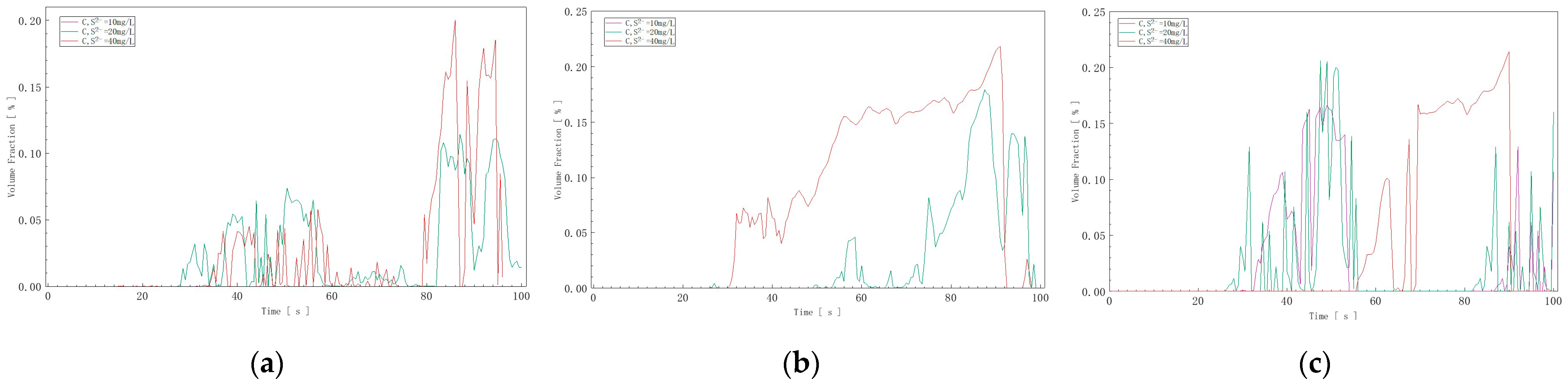
As shown in Figure 10 (Monitoring points are marked with yellow crosses), a monitoring point was set at the top to obtain the curve of the hydrogen sulfide gas concentration at this point over time. This corresponded to the actual laboratory experiment detection location (see Figure 8 for the position of the gas detector in the experiment).

Figure 10.
Monitoring points in the simulation model.
Based on the curves exported from ANSYS 2021 R2 (Figure 11), as seen in Figure 11a, with an inflow velocity of 0.05 m/s, the sulfur ion volume fraction released into the air and reaching the monitoring point was 0.05% at a sulfur ion concentration of 10 mg/L in water, 0.1% at 20 mg/L, and 0.18% at 40 mg/L. In Figure 11b, with an inflow velocity of 0.075 m/s, the sulfur ion volume fraction was 0.06% at 10 mg/L, 0.15% at 20 mg/L, and 0.20% at 40 mg/L. In Figure 11c, with an inflow velocity of 0.1 m/s, the sulfur ion volume fraction was 0.08% at 10 mg/L, 0.18% at 20 mg/L, and 0.22% at 40 mg/L.
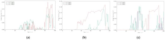
Figure 11.
Hydrogen sulfide volume fraction curves at three different inflow speeds: (a) V = 0.05 m/s; (b) V = 0.075 m/s; (c) V = 0.1 m/s.
Based on the charts and data analysis, it was evident that as the flow rate and concentration increased, the hydrogen sulfide concentration reaching the monitoring point also increased. This demonstrates that during vigorous water movement, the degassing effect of the water increases with the concentration of sulfur ions in the water. Comparing the data at the monitoring point with the initial concentration, the degassing rate of hydrogen sulfide was determined to be 0.05% to 0.22%.
3.3. Experimental Analysis of Hydrogen Sulfide Gas Release
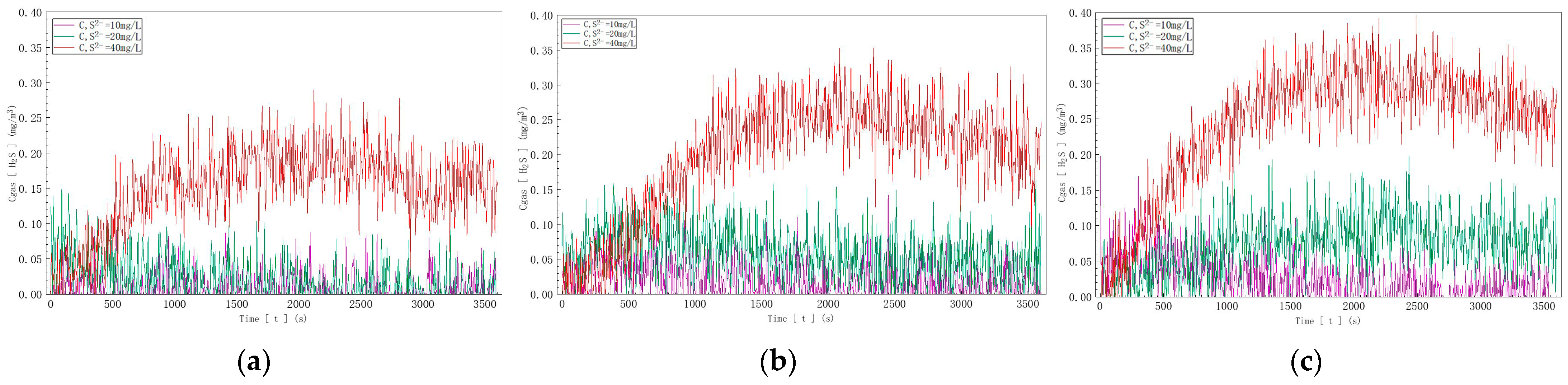
The experiment utilized a gas detector for measurement. To prevent large amounts of hydrogen sulfide gas from being released into the air and affecting the data, the gas detector was placed in a sealed box, which was connected to an opening at the top of the shaft with a gas transmission tube.
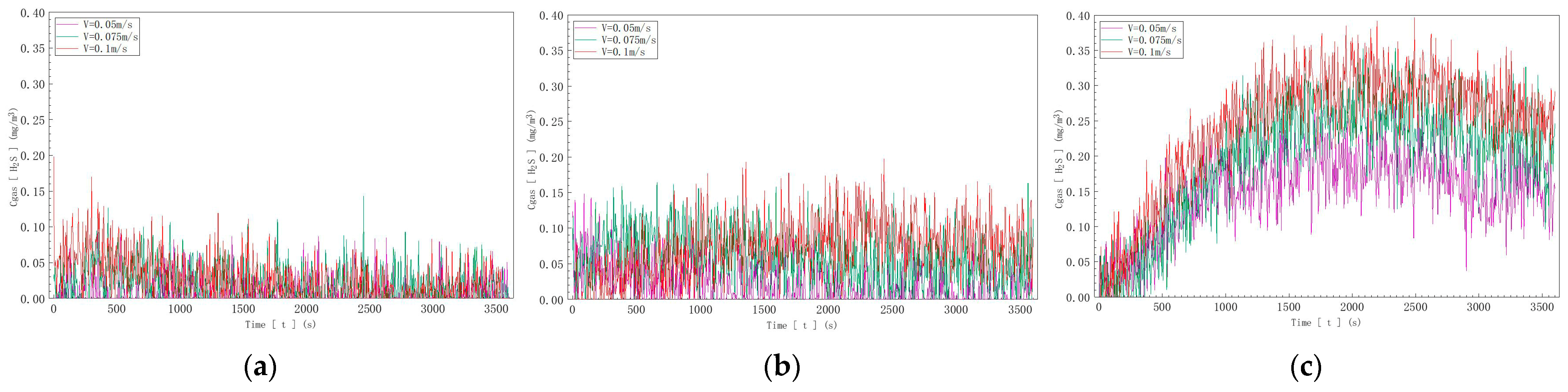
The gas detector data are shown in Figure 12. In Figure 12a, with an inflow velocity of 0.05 m/s and a sulfur ion concentration of 10 mg/l in water, the hydrogen sulfide concentration measured by the gas detector fluctuated between 0.01 mg/m3 and 0.09 mg/m3. At a sulfur ion concentration of 20 mg/L, it fluctuated between 0.03 mg/m3 and 0.14 mg/3, and at 40 mg/L, it fluctuated between 0.05 mg/m3 and 0.27 mg/m3. In Figure 12b, with an inflow velocity of 0.075 m/s, the measured hydrogen sulfide concentration fluctuated between 0.02 mg/m3 and 0.12 mg/m3 at 10 mg/L, between 0.05 mg/m3 and 0.16 mg/m3 at 20 mg/L, and between 0.06 mg/m3 and 0.35 mg/m3 at 40 mg/L. In Figure 12c, with an inflow velocity of 0.1 m/s, the measured hydrogen sulfide concentration fluctuated between 0.03 mg/m3 and 0.15 mg/m3 at 10 mg/L, between 0.07 mg/m3 and 0.19 mg/m3 at 20 mg/L, and between 0.07 mg/m3 and 0.40 mg/m3 at 40 mg/L.
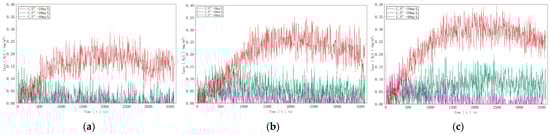
Figure 12.
Hydrogen sulfide concentration curves at three different inflow speeds: (a) V = 0.05 m/s; (b) V = 0.075 m/s; (c) V = 0.1 m/s.
In summary, it is known that under the same velocity conditions, the concentration of hydrogen sulfide gas released into the air increases with the increase in sulfur ion concentration in the water. This demonstrates that at a determined pH value, the degassing rate of water increases with the increase in sulfur ion concentration in the water.
According to the data depicted in Figure 13, in Figure 13a, with a sulfur ion concentration of 10 mg/L, the hydrogen sulfide gas concentration detected reached a maximum of 0.15 mg/m3 as the inflow velocity increased; in Figure 13b, with a sulfur ion concentration of 20 mg/L, the detected hydrogen sulfide gas concentration reached a maximum of 0.20 mg/m3 as the inflow velocity increased; and in Figure 13c, with a sulfur ion concentration of 40 mg/L, the detected hydrogen sulfide gas concentration reached a maximum of 0.40 mg/m3 as the inflow velocity increased.

Figure 13.
Hydrogen sulfide concentration curves at three different sulfide ion concentrations: (a) C, S2− = 10 mg/L; (b) C, S2− = 20 mg/L; (c) C, S2− = 40 mg/L.
In summary, for solutions with identical sulfur ion concentrations, the concentration of hydrogen sulfide gas released into the air increases with the increase in water inflow velocity. This demonstrates that at a determined pH value, the degassing rate of water increases with the increase in water inflow velocity.
In summary, and based on the comparison between the detection location data and initial concentration calculations, the degassing rate of hydrogen sulfide was determined to be 0.1–0.4%.
Based on the above analysis, the study indicates that with the increase in flow rate and the concentration of sulfide ions in the water, the concentration of hydrogen sulfide gas reaching the monitoring point significantly rises. This phenomenon suggests that during vigorous water movement, the degassing effect of the water intensifies with the increase in sulfide ion concentration. Compared to previous studies, our experimental results further validate the behavior of hydrogen sulfide transport and release in flowing water bodies. While existing research has shown that hydrogen sulfide release is closely related to water pH and sulfide ion concentration, this study particularly highlights the significant impact of increased flow rate on the degassing efficiency at the same sulfide ion concentration. However, despite these results providing critical insights into the release mechanism of hydrogen sulfide, controlling its release in real-world environments still requires further investigation. Future studies could explore optimizing hydrogen sulfide control strategies by adjusting the water pH, flow rate, and sulfide ion concentration as well as introducing chemical inhibitors. These control measures could not only reduce hydrogen sulfide emissions, but also mitigate potential environmental impacts, offering more effective solutions.
4. Conclusions
This paper focused on a shaft project in St. Petersburg and innovatively introduced a spiral tray structure into the design. Detailed simulation experiments were conducted using ANSYS finite element analysis to assess the impact of the spiral tray on the hydrogen sulfide degassing rate. The simulation results indicated that the degassing rate of hydrogen sulfide fluctuated between 0.05% and 0.22%. To further validate the reliability of the simulation, a proportional experimental model was constructed in the laboratory, where systematic testing determined the hydrogen sulfide degassing rate to be between 0.1% and 0.4%.
The findings revealed that as the concentration of sulfide ions in water increases, the rate at which hydrogen sulfide is released into the shaft significantly rises. Additionally, an increase in the inflow velocity of water also accelerates the hydrogen sulfide release rate. This phenomenon was not only confirmed under laboratory conditions, but also observed during actual shaft operations. Therefore, by controlling the concentration of hydrogen sulfide in the water and reducing the turbulence of the water flow during real-world shaft operations, the release of hydrogen sulfide can be effectively minimized, thereby enhancing the efficiency and safety of the shaft’s operation.
The results of this study are of significant theoretical importance and demonstrate broad practical application prospects. By appropriately adjusting the design parameters of the shaft, such as controlling the water flow velocity and sulfide ion concentration, the safe and stable operation of the shaft can be ensured while significantly reducing the negative impact of hydrogen sulfide on the surrounding environment and human health. These findings provide a robust scientific basis for optimizing the design and operation of shaft projects, and can be applied to similar engineering projects.
More importantly, this study revealed the potential contribution of shaft projects to achieving sustainable development goals. By effectively reducing hydrogen sulfide emissions, this research not only helps to mitigate the environmental impact of engineering projects, but also offers practical solutions for reducing air pollution and protecting the ecological environment. These research outcomes are not only widely applicable in the field of shaft engineering, but also provide important references for the design, construction, and operation of other similar infrastructure projects. This innovative integration of design and environmental protection represents the future direction of engineering technology development and offers new ideas and methods for achieving sustainable development goals.
Funding
This research received no external funding.
Data Availability Statement
The raw data supporting the conclusions of this article will be made available by the authors on request.
Acknowledgments
First and foremost, I extend my heartfelt gratitude to Fedorov Svyatoslav Viktorovich. His guidance and support have been invaluable both academically and personally. Throughout the entire process of selecting my thesis topic, conducting the experimental research, and writing my dissertation, his dedication and insight have been profoundly influential. His integrity, rigorous scholarly approach, and patient instruction have left an indelible mark on me, shaping my future work and life profoundly. I also wish to express my deep appreciation to the professors who assisted in the writing and reviewed my thesis, taking time out of their busy schedules to provide their expertise. I extend my sincerest respect and gratitude to them. Finally, I am deeply thankful to my parents for their unwavering support and selfless love, enduring great hardships to ensure my growth and success.
Conflicts of Interest
The authors declare no conflict of interest.
References
- Xing, Y.; Cao, X.; Liu, T.; Xu, G.; Yang, C.; Lu, C.; He, J. Current Status, Problems, and Development Suggestions of Urban Drainage Systems in China. China Water Wastewater 2020, 36, 19–23. [Google Scholar]
- Li, H.; Zhang, L.; Tang, X.; Chen, W. Analysis of the Causes and Influencing Factors of Hydrogen Sulfide Gas Production in Urban Drainage Pipelines. Environ. Sci. Manag. 2012, 37, 95–97+107. [Google Scholar]
- Sun, H.; Hao, Y.; Long, T. Drainage Engineering (Volume I); China Architecture & Building Press: Beijing, China, 1999; pp. 1–3. [Google Scholar]
- Xu, W. Study on the Overflow Law of H_2S in Urban Sewage Drainage Systems. Master’s Thesis, Lanzhou University of Technology, Lanzhou, China, 2014. [Google Scholar]
- Su, S.; Yang, X.; Chen, S.; Peng, S. Study on Methane Explosion in Urban Sewers. Urban Gas 2021, 153–157. [Google Scholar]
- Hu, W.; Du, Y. Hazards and Detection Methods of Hydrogen Sulfide Gas. Materials Prot. 1996, 29, 17–18. [Google Scholar]
- Zhu, Y.; Wang, X.; Zhang, L.; Zhang, J. Hazards and Preventive Measures of Hydrogen Sulfide in Drainage Systems. China Water Wastewater 2000, 16, 45–47. [Google Scholar]
- Zhang, Y. Experimental Study on Methane Chlorination Reaction with Pulsed Corona Plasma. Master’s Thesis, Zhejiang University of Technology, Hangzhou, China, 2009. [Google Scholar]
- Robert, W.; Seabloom, P.E. Emeritus Professor of Civil and Environmental Engineering Dept. of Civil and Environmental Engineering. Septic Tank; Ted Loudon Professor of Agricultural Engineering Farall Hall.
- Li, H. Analysis of Key Points in the Design of Municipal Drainage Networks. Urban Archit. Space 2023, 30 (Suppl. S2), 197–198. [Google Scholar]
- He, J. Analysis of Construction and Operation Problems of Urban Drainage Networks. Urban Constr. Theory Res. (Electron. Ed.) 2022, 142–144. [Google Scholar]
- Chen, W.; Wu, Z.; Xu, C.; Bian, G.; Ma, Z.; Dai, L. CFD-Based Design and Energy Dissipation Analysis of Vertical Drop Shaft Structures. Software 2020, 41, 170–174. [Google Scholar]
- Lin, B. Planning and Optimization Design of Municipal Drainage Networks. Eng. Technol. Res. 2022, 7, 181–182. [Google Scholar]
- Chen, Z.; Wei, H.; Qin, J. Research on Large Drop Shaft Model Tests in Shanghai Drainage Projects. J. Northwest Inst. Archit. Eng. (Nat. Sci. Ed.) 2000, 69–75. [Google Scholar]
- Wu, H.; Ma, N. Model Test Research on Energy Dissipation Effect of Drop Shafts. J. Chongqing Univ. 2022, 45 (Suppl. S1), 111–114. [Google Scholar]
- Wang, L.; Guo, J.; Wei, J.; Liang, R. Application Research of Vertical Shaft Structures in Urban Drainage Systems. J. Lanzhou Petrochem. Vocat. Coll. 2022, 22, 23–26. [Google Scholar]
- Ma, Y. Research on Gas Entrainment and Energy Dissipation in Drop Structures of Drainage Systems. Ph.D. Thesis, Zhejiang University, Hangzhou, China, 2016. [Google Scholar]
- Ding, C. Research on the Movement and Distribution of Harmful Gases in Sewage Pipelines. Master’s Thesis, Xi’an University of Architecture and Technology, Xi’an, China, 2015. [Google Scholar]
- Lu, S.; Qiao, S. Optimization and Numerical Simulation of Pressure Characteristics of Vertical Drop Shaft Structures. Adv. Water Sci. Technol. 2023, 43, 24–29+43. [Google Scholar]
- Liu, C. Numerical Simulation of Energy Dissipation in Vertical Shaft Flood Discharge Tunnels Based on CFD. Hydraul. Sci. Cold Reg. Eng. 2022, 5, 10–13. [Google Scholar]
- Gao, M. Hydraulic Characteristics Simulation Analysis of Vertical Swirling Flood Discharge Shaft Based on FLUENT. Shaanxi Water Resour. 2022, 4–8. [Google Scholar] [CrossRef]
- Yao, Y. Experimental Study on Hydraulic Characteristics of Deflector Plate Type Deep Tunnel Vertical Shaft Energy Dissipation. Master’s Thesis, Southwest Jiaotong University, Chengdu, China, 2020. [Google Scholar]
- Vallet, A.; Burluka, A.A.; Borghi, R. Development of a Eulerian model for the “Atomization” of a liquid jet. At. Sprays 2001, 11, 619–642. [Google Scholar] [CrossRef]
- Wu, P. Numerical Simulation Study of a New Energy Dissipation Device for Horizontal Swirling Flow in Vertical Shafts. Master’s Thesis, Hefei University of Technology, Hefei, China, 2010. [Google Scholar]
- Lu, J.; Ding, C. Verification of a Mathematical Model for Ventilation in Sewage Pipelines Based on CFD. China Water Wastewater 2014, 30, 67–70. [Google Scholar]
- Li, L.; Xie, M.; Jia, M. Numerical Analysis of Different Turbulence Models for Sprays Using the New Euler Model. J. Intern. Combust. Engines 2018, 36, 76–82. [Google Scholar]
- Zhu, D.; Gu, P.; Chu, H.; Lin, F.; Lu, S. Numerical Study on the Layout and Optimization of Airflow Organization in the Grate Room of Sewage Pumping Stations. J. Nanjing Norm. Univ. (Eng. Technol. Ed.) 2019, 19, 43–49+81. [Google Scholar]
- Gao, W.; Ma, L.; Zhu, X.; Li, S.; Jiang, X. Non-Isothermal Thermal Decomposition Kinetics of Acrylic Artificial Stone Waste Powder/ABS Composites. Plastics 2024, 53, 52–57. [Google Scholar]
- Zheng, S.; Li, W.; Yang, H.; Chen, S.; Wei, Q. Research and Application Progress on the Modification of 3D Printed Polylactic Acid. Mater. Rev. 2024, 38, 256–265. [Google Scholar]
- Teng, Y. Dissolution Behavior of Hydrogen Sulfide in Water. Arid. Environ. Monit. 1994, 11–13+60. [Google Scholar]
- Zhang, L.; De Schryver, P.; De Gusseme, B.; De Muynck, W.; Boon, N.; Verstraete, W. Chemical and biological technologies for hydrogen sulfide emission in sewer systems: A review. Water Res. 2008, 42, 1–12. [Google Scholar] [CrossRef] [PubMed]


Disclaimer/Publisher’s Note: The statements, opinions and data contained in all publications are solely those of the individual author(s) and contributor(s) and not of MDPI and/or the editor(s). MDPI and/or the editor(s) disclaim responsibility for any injury to people or property resulting from any ideas, methods, instructions or products referred to in the content. |
© 2024 by the author. Licensee MDPI, Basel, Switzerland. This article is an open access article distributed under the terms and conditions of the Creative Commons Attribution (CC BY) license (https://creativecommons.org/licenses/by/4.0/).