Abstract
Several cities are facing an increasing flood risk due to the coupled effect of climate change and urbanization. Non-structural protection strategies, such as Early Warning Systems (EWSs), have demonstrated significant potential in mitigating hydraulic risk and often become the primary option when the implementation of structural measures is impeded by the complexities of urban environments. This study presents a new EWS designed specifically for fluvial floods in the city of Palermo (Italy), which is crossed by the Oreto River. The system is based on the preliminary definition of various Flood Event Scenarios (FESs) as a function of typical precursors, such as rainfall forecasts, and antecedent wetness and river flow conditions. Antecedent conditions are derived from real-time water stage observations at an upstream river section, while rainfall forecasts are provided by the Italian National Surveillance Meteorological Bulletins with a preannouncement time of up to 36 h. An innovative feature of the system is the use of rainfall Depth–Duration Thresholds to predict the expected hydrograph peak, significantly reducing warning issuing times. A specific FES, immediately accessible from a pre-built library, can be linked to any combination of precursors. Each FES predicts the timing and location of the first points of flooding; flood-prone areas and water depths; and specific hazard maps for elements typically exposed in cities, such as people, vehicles, and buildings. The EWS has been tested on a historical flood event, demonstrating satisfactory accuracy in reproducing the location, extent, and severity of the flood.
1. Introduction
According to a recent report by the European Commission [1], damage caused by natural disasters in Europe from 1980 to 2017 exceeded 500 million euros, 90% of which was due to rare and intense meteorological events for which an early warning had not been issued and no adequate spatial planning measures had been taken.
Ongoing climate change is leading to an intensification of meteorological events and an increase in the frequency of extreme events, especially in some hot-spots of the Mediterranean basin [2]. Moreover, the progressive expansion of urbanized areas on a global scale [3] has deeply modified land use and the density of the elements that are exposed to flood hazards in urban settlements. The increment of impervious surfaces implies alterations to the processes of generation and propagation of surface runoff, typically exacerbating the impacts of rainfall on the ground; this is mainly due to the reduction of infiltrated water, with faster generation and routing of surface runoff, along with higher stormwater volumes and peak flows [4]. All this could severely stress the urban natural and artificial drainage systems and trigger unprecedented catastrophic phenomena of urban pluvial and fluvial floods.
Hydraulic risk reduction strategies are urgently needed, especially in areas particularly affected by climate change and already vulnerable to flood risks, such as Italy, where there is clear evidence [5] of the extreme weakness of the territory, with approximately 12% of the national population (i.e., over 7 million inhabitants) living in areas classified at significant flooding risk (i.e., from “moderate” to “very-high” according to the national risk classification, aligned with the Floods Directive 2007/60/EC).
The United Nations International Strategy for Disaster Reduction [6] reported some risk reduction efforts undertaken across the world, identifying ten practices referred to as “essentials” supporting each of them. “Essential 9” (effective preparedness, early warning, and response) highlights the importance of strengthening non-structural preparedness measures to ensure that cities, communities, and individuals can act appropriately to reduce the threats posed by natural and human-induced disasters. From this perspective, Early Warning Systems (EWSs) are low-cost and adaptive non-structural protection measures for the reduction in flood impacts in urban areas [7].
The typical architecture of an EWS consists of four key components [8]:
- Risk knowledge through the identification of hazards, exposures, and vulnerability;
- Forecasting and monitoring of hydro-meteorological variables, such as water stage, flow velocity, and rainfall and data processing using computational models;
- Dissemination and communication of alerts;
- Reaction to the alerts issued.
One of the main features of an EWS is the time required to issue the alert; in small basins (e.g., <100 km2), preannouncement activity must be based on medium–high temporal prediction horizons, referring to forecasting and/or nowcasting activities rather than real-time monitoring. The use of forecasts in EWSs finds further difficulties due to possible limitations of the forecasting models, which often fail to simulate events with reduced space-time scales [9]; current meteorological models can accurately predict events occurring in a temporal window of 24–48 h over large portions of territory (e.g., >100 km2) [10].
In nowcasting, the major issues involve the need for limited execution times required for the EWS during (i) event monitoring to correct the Quantitative Precipitation Forecasts (QPFs) via real-time data assimilation [11], (ii) hydrological–hydraulic processing using computational models, (iii) population reaction to alerts. Different forecasting schemes for pluvial flash floods based on QPFs were presented in [12], including susceptibility assessment (i.e., flooding is linked to specific hydrometeorological precursors like rainfall depth, relative humidity, basin soil moisture); rainfall comparison with surface conditions neglected (i.e., flooding occurs when QPF exceeds specific rainfall thresholds, obtained from statistical analyses on historical precipitation data [13,14]) or with surface conditions considered (similar to the previous but includes thresholds obtained from hydrological modelling [15,16]); flow comparison (i.e., expected flow rate, determined from QPF via hydrological modelling, is compared with threshold values, obtained through hydrological simulations [17] or statistical analyses [18]).
Weather forecasts can be performed using three methodologies [13]: radar-based models, numerical weather predictions, or blending products. Probabilistic and deterministic radar-based models are mainly used in nowcasting [19,20,21]. Numerical weather predictions are used both in nowcasting and forecasting. Generally, outputs require dynamic (LAM, Limited Area Model) or statistical downscaling (e.g., the rainFARM model [22] to increase the spatial resolution). Integrated approaches can also be used [23]. Finally, both LAM models and ground-based measurements with remote sensors or meteorological radar are used for blending products [24].
In some cases, EWSs are based on the construction of offline libraries of Flood Event Scenarios [23,25,26], linking rainfall forecasts to hazards and expected damages. Through the exploration of different simulated scenarios, it is possible to define a relationship between event precursors, elements exposed to flood risk, and the potential damages.
The present study proposes a novel EWS for urban fluvial floods developed for the focal area of the Oreto River, which crosses the city of Palermo (Italy). Although the system was developed considering the peculiarities of the case study, the general framework is easily transferrable and replicable in other territorial contexts and complex urban areas.
A pre-built library of Flood Event Scenarios (FESs) was preliminarily developed to characterize the relationship between flood precursors and associated potential hazards. To this aim, a hydrological study was carried out using the model HEC-HMS (Hydrological Modeling System) [27], determining a set of design hydrographs with predefined peak values (Qpeak,FES). The hydraulic propagation of all design hydrographs within the computational domain was simulated using the open-source calculation code HEC-RAS (River Analysis System) [28], considering different initial conditions (Qinit,FES) and obtaining a total of 76 FESs. Each FES, associated with a given pair of Qpeak,FES and Qinit,FES values, provides the timing and location of potential first points of flooding, the flood area extension with the maximum expected water depths, and specific hazard maps for three typologies of elements typically exposed to the flood hazard in urban areas, i.e., people, vehicles, and infrastructures. The Flood Directive 2007/60/CE highlights the importance of considering hydrodynamic factors that can characterize flood evolution in the hazard assessment, explicitly referring to flow velocities. Flow velocity is strictly related to some important potential damaging actions of floods in urban areas since it influences hydrodynamic pressures, erosion processes, buoyancy forces, and debris flow. The scientific literature has developed various contributions useful for the definition of criteria for the classification of vulnerability and/or damage in relation to the types of elements exposed to risk; most of them, including those adopted for this study, consider the combined effect of water level and flow velocity. Some criteria and adopted indicators for the evaluation of human, vehicle, and building stability under the influence of flood actions can be found, for example, in [29,30,31,32,33,34,35,36,37,38]. An important aspect in the generation of the FES library for the proposed EWS was the high-resolution definition of the computational domain. This was obtained from a Digital Elevation Model (DEM) with a spatial resolution of 2 m, opportunely ground-corrected to account for the geometries of bridges, buildings, and other infrastructures potentially influencing the surface runoff routing.
The approach adopted, based on an offline library of FESs, offers the significant advantage of enabling rapid alert issuance, thereby serving as an effective decision-support tool for civil protection systems during both the planning and emergency management phases. For instance, the prediction of a given FES in response to rainfall forecast allows for localizing potential hazards and planning consequentially appropriate civil protection actions at the local level during the emergency phase, such as the inhibition of pedestrian and/or vehicular transit on some roads and underpasses and the issuing of warnings to the population.
The case study, the EWS, and the general framework are defined in the first part of the paper (Section 2). In particular, the EWS relies on (i) a rainfall forecast system; (ii) real-time river stage observations recorded by a water stage gauge station located in an upstream section of the river; (iii) rainfall Depth–Duration–Frequency (DDF) and Depth–Duration Thresholds (DDTs) curves, with these last defined for the basin under analysis in a previous work [39]. Rainfall forecasts and initial river flow conditions are herein considered potential flood event precursors. Expected rainfall is obtained from the 36 h QPF provided daily by the Italian National Surveillance Meteorological Bulletins (NMBs), deriving an expected rainfall trajectory based on DDF curves. The expected hydrograph peak is assessed by combining the obtained rainfall trajectory with the numerical rainfall DDTs. River stages, monitored in real-time by the Oreto at Ponte Parco (OPP) hydrometric station, are used to estimate the initial river flow condition (Q0).
The use in real-time of the EWS consists of the following procedural steps:
- Acquiring the NMB and the associated maximum expected cumulative depth and accumulation period from the QPF to derive the expected rainfall trajectory;
- Retrieving the water stage at the OPP station at the time of issuing of the NMB, assessing Q0, and identifying 1 out of 10 possible reference families of iso-critical discharge DDT curves (Qinit,DDT);
- Deriving the expected hydrograph peak flow from the DDTs (Qpeak,DDT) based on the rainfall trajectory (point 1) and the selected reference family of DDT curves (point 2);
- Associating Q0 (point 2) with one out of four possible initial discharge conditions (Qinit,FES) considered for the generation of the FES library;
- Associating Qpeak,DDT (point 3) with 1 of the 19 possible peak values (Qpeak,FES) considered for the generation of the FES library;
- Retrieving from the library the expected FES associated with the paired Qinit,FES − Qpeak,FES values.
An analysis of the fluvial flood risk in the study area based on the outcomes of the FES library is discussed in Section 3, also proposing possible urban planning measures that could be associated with specific FESs. The EWS was also tested with respect to a historical flood event that occurred in 2018, demonstrating satisfactory performance in terms of predicted flood area extension and associated water depths, as reported in Section 3. A discussion section and some concluding remarks conclude the paper.
2. Materials and Methods
2.1. Study Area: The City of Palermo and the Oreto River Basin
Palermo is the largest (160 km2) and most populated (855,000 inhabitants) city in Sicily, southern Italy. The city is noted for its history, culture, and architecture, with innumerable monuments and goods of inestimable value and a particularly active economic tissue. According to [40], Palermo was the sixth most vehicular traffic-congested city in the world in 2022. All this contributes to making Palermo particularly exposed to flood risk.
The original hydrographic configuration of the city has been completely changed over the years; two rivers that originally crossed the city (i.e., the Kemonia and the Papireto rivers) have been forced underground, and the only river still flowing on the surface is the Oreto. The hydrographic basin of the Oreto River (Figure 1) has an extension of about 110 km2. It extends southwest of the urban area of Palermo and is surrounded by the Pioppo, Monreale, and Altofonte hills. The hydrographic network is composed of two main tributaries that drain the water from two sub-basins (SB1 and SB2 in Figure 1) and converge close to the Ponte Corleone bridge. The Input Control Section (ICS) for the reference area of the proposed EWS is located slightly downstream of this bridge.

Figure 1.
Oreto River Basin. (a) Indications of the two contributing sub-basins (SB1 and SB2), the computational domain (red contour) for the EWS, the location of the six bridges crossing the river (from 1 to 6), the Palermo–SIAS rain gauge, the Oreto a Ponte Parco hydrometric station (OPP), and the Input Control Section (ICS) for the hydraulic modelling. Righthand boxes show the different domains considered to calculate the hazard maps for (b) people, (c) vehicles, and (d) buildings.
The Ponte Parco bridge, which is located at the OPP hydrometric station, is within the larger sub-basin SB1. The OPP station, supporting the river monitoring telemetry system of the Basin Authority of the Sicilian Regional District (Autorità di Bacino della Regione Sicilia, hereafter AdB), is located 10 km upstream of the outlet at elevation of 608 m a.s.l., and it has a drainage area of 77 km2; it has collected data since 1921, and it also includes an ultrasonic water stage telemetry sensor, recently installed.
The sub-basin SB2 originates from the Boccadifalco’s artificial channel, which was realized after the catastrophic fluvial flood of 1931. Downstream of the ICS, the river crosses the city for about 5.5 km before flowing into the Tyrrhenian Sea. It has meandering shapes with steep and incised banks within calcarenites. The final part of the river has been regularized by building a spillway and it was subjected to floodplain modifications with concrete coverage and the creation of vertical walls. This stretch of the river is crossed by six bridges, whose location is also reported in Figure 1a: (1) the railway bridge of the Palermo-Trapani line; (2) a walkway (corner via Guadagna-via Paternò); (3) the road bridge of via Oreto; (4) the railway bridge of the Palermo–Agrigento line; (5) the road bridge of Corso dei Mille; (6) the road bridge of via Messina Marine.
Palermo has a Mediterranean climate with hot and dry summers and cold and wet winters. The average annual temperature is about 22 °C, while the annual average precipitation is about 800 mm, mainly concentrated in autumn and winter. In the last years, the city has experienced some extreme rainfall events, usually concentrated at the end of summer, which have frequently caused severe pluvial floods. The Oreto River has flooded more than 30 times since 1912, with the last event, herein considered to test the proposed EWS, recorded in November 2018.
2.1.1. Flow Rating and Flow Duration Curves at OPP
The Flow Rating Curve (FRC) and the Flow Duration Curve (FDC) derived at the OPP are used for the development of the proposed EWS. The FRC indicates the stage–flow relationship for a specified section of interest; it is usually reconstructed based on a large dataset of paired measures of discharge and river stage collected in different periods of the year. Since cross-sections may vary over time due to vegetation growth and riverbed movements, FRCs typically require periodic recalibrations. The FDC provides a representation of the streamflow frequency distribution, describing the basin attitude to provide flows of various magnitudes and offering a simple yet comprehensive, graphical view of the streamflow regime and variability [41]; it is usually derived from long (e.g., >20 years) historical time series of observed daily streamflow and, although the FDCs are less variable in time than the FRC, period updating should also be performed.
Part II of the official AdB Annual Reports (i.e., Annali Idrologici, available online at the ISPRA web portal: http://www.bio.isprambiente.it/annalipdf/; accessed on 5 July 2024) provides measurements of river stage and discharge, FRCs, and historical FDCs for the main Italian river basins. Data at the OPP are available from 1921 to 1997 and refer to the old manual water stage gauge, replaced by the new telemetric sensor in 2012; the last available FDC in the Annual Reports dates to 1941.
In this study, we considered an updated FRC, derived in 2022 within a scientific collaboration agreement between the Department of Engineering of the University of Palermo and the AdB (Figure 2a), whose analytical expression is given by
where Q is the discharge (m3/s) and HAdB is the water stage (m) recorded by the telemetric sensor at the OPP.
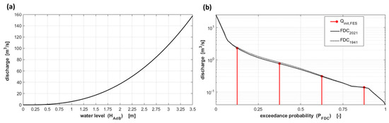
Figure 2.
(a) Flow Rating Curve (FRC) and (b) Flow Duration Curve (FDC2021) derived at the OPP. For the FDC, the discharge is reported in logarithmic form, and vertical grid distinguishes the four different streamflow conditions considered for the FESs generation, with the values of streamflow associated with each class (Qinit,FES = QLF, QLM, QMH, and QHF) highlighted in red. The old version of the FDC (FDC1941) is also reported for comparison (black dashed curve).
A new version of the FDC at the OPP (FDC2021), referring to the period up to 2021, was herein considered; it was derived using all the available daily streamflow data from the Annuals and the recent stage data from the telemetric sensor, opportunely converted in streamflow by Equation (1). According to the FDC (Figure 2b), the ordinary flood (i.e., Q91) and drought (Q274) thresholds were equal to 1.28 and 0.19 m3/s, respectively, while the semipermanent flow (i.e., Q185) was equal to 0.54 m3/s.
These values, representing the quartiles of the FDC, are herein used to classify the initial streamflow at the OPP (Q0) according to four classes, considered proxy measures of the basin’s antecedent wetness conditions: (i) low flow, LF (i.e., Q0 < Q274); (ii) low–medium flow, LM (i.e., Q274 ≤ Q0 < Q185); (iii) medium–high flow, MH (i.e., Q185 ≤ Q0 < Q91); high flow, HF (i.e., Q0 ≥ Q91). In particular, the central value of each range is associated with each class so that, for example, the streamflow value, QLF, associated with all values of streamflow within the LF class, is equal to the 87.5th percentile of the FDC, as described in Table 1. The four values (QLF, QLM, QMH, and QHF) were used as alternative initial river flow conditions at the OPP for the generation of the FES library, and thus, they provide one of the two label values (i.e., Qinit,FES) required to identify the expected FES at a given time. The initial discharge observed at the OPP (Q0) not only determines Qinit,FES but is also utilized to identify the reference family of iso-critical discharge DDT curves, as will be discussed in detail in Section 2.2; consequently, it also contributes to determining the other label value (i.e., Qpeak,FES) necessary for identifying the expected FES.

Table 1.
Classification of the initial discharge, Q0, at the OPP, with the associated initial condition for the FES identification in terms of discharge (Qinit,FES) and exceedance probability from the FDC2021 (PFDC,2021). Values of initial discharge at the OPP (Qinit,DDT) are associated with the ten different families of iso-critical discharge DDT curves derived in [39].
2.1.2. Characterization of the Computational Domain
The reference area for the proposed EWS is located within the historic centre of Palermo, a district with a very high population density and a large presence of highly vulnerable sites, such as hospitals, schools, public offices, basement flats, economic activities, and shops. The area also includes a Natura 2000 Site of Community Importance (SCI: ITA 020012 Valle del Fiume Oreto). A characterization of the hydraulic risk for the study area is given by the Hydrogeological Setting Plan (Piano stralcio per l’Assetto Idrogeologico—PAI) for Sicily, which is the official regional plan mapping the hydraulic and geomorphological hazards and risks. The PAI of this area, which was elaborated in the early 2000s and updated in 2018, shows many areas classified with “high” (class R3) and “very high” (class R4) hydraulic risk.
The hydraulic domain (Figure 1 and Figure 3) covers a surface of 1.77 km2, and it was derived from a DEM with a spatial resolution of 2 m, provided by the Sicilian Region, appropriately edited and corrected by digitalising the built-up elements, such as river embankments, bridges, buildings, roads, railways, walls, underpass roads, traffic islands, sidewalks, curbs, and any other elements potentially influencing flow direction within the study area (Figure 3). To this aim, technical documents provided by the Municipality of Palermo, as well as the results of on-site and remote inspections via Google Earth, were considered. The exact geometry of the bridges, which may potentially affect the streamflow during extreme flooding events, was reconstructed using the original project documents (insets in Figure 3).
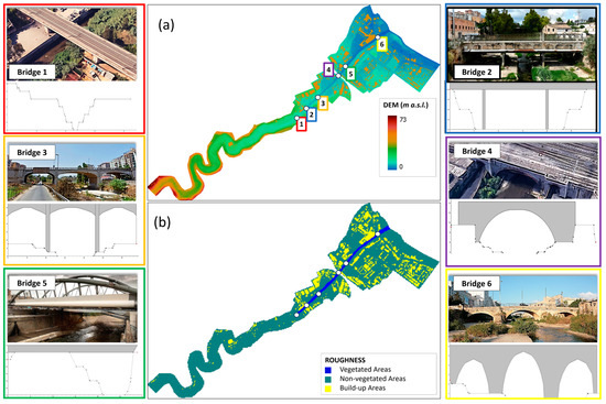
Figure 3.
Computational hydraulic domain: maps of (a) elevation and (b) roughness. Locations of the bridges are also indicated, while their geometry is depicted in the insets.
The computational mesh generated includes a total of 32,691 cells having a regular spatial resolution of 2 m; a variable and more detailed resolution has been used to describe the elevation discontinuity due to elements such as river embankments and walls. A very high, artificial elevation (i.e., 40 m a.s.l.) was assigned to the buildings’ footprints so that the model perceives these elements as “virtual walls”, thus forcing surface runoff to flow around them (Figure 3a).
In terms of roughness, the domain was classified into two homogeneous sub-areas (Figure 3b): vegetated areas, mainly including the riverbed and riverbank, and non-vegetated areas. Values of Manning’s roughness coefficient assigned to the vegetated and non-vegetated areas are 0.03 and 0.04 s m−1/3, respectively, and were retrieved from [42].
Two sub-domains, displayed in Figure 1 and derived from specific maps provided by the Municipality of Palermo, are considered for mapping the hazard for vehicles and buildings, respectively. In particular, the first (Figure 1c) considers only the roads and streets within the main domain, while the second (Figure 1d) considers a buffer zone of 3 m width around the buildings.
2.2. Rainfall Depth–Duration Thresholds
A rainfall Depth–Duration Threshold (DDT) for flood warning is usually defined as the rainfall threshold for a given duration over which a critical discharge is exceeded in a given river section [17,43,44,45]. DDT relies on the hydrological initial conditions of the basin and the rainfall features, i.e., duration, intensity, and shape of the hyetograph. The critical discharge is typically representative of flow conditions beyond which phenomena of hydraulic insufficiency and consequent floods are triggered; in this case, the rainfall threshold can be thought of as the maximal sustainable rainfall for a basin.
Different rainfall DDTs at the OPP river basin were derived through a deterministic approach in [39]. The thresholds were numerically estimated using the TOPDM hydrological model [46], considering different rainfall durations and different combinations of initial basin saturation conditions and storm shapes to obtain the amount of rainfall causing critical flow at the basin outlet. The DDTs were provided in the form of parametric iso-critical discharge curves on a cumulative rainfall, Ec, and duration, d, plot. In particular, after the simulation of the basin, hydrological response for a total of about 16,000 rainfall events with fixed cumulative value, duration, initial soil moisture, and hyetograph type, different families of iso-critical discharge curves on Ec-d plots were obtained. Each plot is specific for a given combination of initial soil moisture and hyetograph type and reports curves associated with critical flow values at the OPP (Qpeak,DDT) up to 1600 m3/s. More specifically, for every possible combination of initial soil moisture and hyetograph type, a total of 528 synthetic rainfall events were considered, ranging from 1 to 24 h and having a cumulative rainfall between 40 and 250 mm. Three possible temporal distributions of the rainfall were considered using the following synthetic hyetograph types: H1, hyetograph with positive gradient; H2, hyetograph with negative gradient; and H3, isosceles triangle hyetograph. Initial soil moisture conditions were taken into account by imposing ten different values of discharge (Qinit,DDT) as contour conditions for the TOPDM simulations; discharges vary from 0.05 m3/s to 7 m3/s (Table 1) and were extracted from the FDC1941 considering exceedance probabilities ranging from 0 to 1 with step 0.1. Thus, a total of 30 (=3 hyetograph types × 10 initial values of discharge) possible contour conditions were considered, generating a total of 30 different Ec-d plots, for which parametric iso-discharge curves (with parameter Qpeak,DDT) were derived by interpolating the obtained maximum discharge values. For more details, interested readers are referred to the original paper [39].
2.3. Flood Event Scenarios: Definition and Products
Flood Event Scenarios (FESs) are tools often used to define the expected hazard level in a specific area after a specific calamitous event [47,48]. FESs can be described with different detail levels. The basic level is based on simplified analyses providing at least a concise description of the areas potentially affected by the event (flooding areas and elements exposed to risks). More detailed levels are usually supported by more complex modelling tools and provide detailed information on the characteristics of the event (flooding areas, water levels, flow velocity, and directions). The flood hazard classification of areas and points within a territory associated with an event of given return period is the main expected product of FESs and represents essential information both in the territorial planning activities, according to the Floods Directive 2007/60/CE, and in the emergency management of risk for civil protection purposes.
In this study, FESs are used with the aim of characterizing the hydrological response of a given area to a forecasted meteorological event and assessing the potential consequences in terms of flood characteristics and hazards. Although each simulated event considered to generate a FES may have a statistical connotation, with a specific return period associated, herein, we explicitly neglect this aspect, considering each FES as the result of the hydraulic propagation of a standard design hydrograph, with known peak flow (Qpeak,FES) and initial conditions (Qinit,FES), over a predefined area.
Each FES is then uniquely identified by paired values of peak flow and initial discharge and includes several products, schematically reported in Figure 4 and described in detail in the following. A large FES library was created considering a set of design hydrographs with different peak flows and initial discharges, according to the procedure that will be fully described in Section 2.5. The modelling chain used allows for simulating the temporal variation of water levels and velocities at all nodes of the computational domain, in response to each hydrograph, under the imposed hydrological and hydraulic boundary conditions.
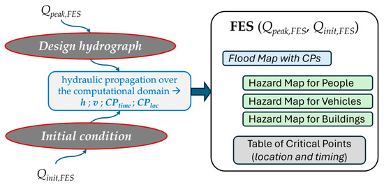
Figure 4.
Schematic representation of a generic FES. Each FES is derived by propagating over the computational domain a standard design hydrograph with given peak flow (Qpeak,FES) and initial discharge (Qinit,FES) and deriving water levels (h) and flow velocity (v) at each node as well as critical flooding points location (CPloc) and timing (CPtime). Each FES provides a report table for the critical points and spatial maps of water levels and hazard maps for people, vehicles, and buildings.
Based on the results of the modelling, the following products, which are deemed fundamental information to plan specific local interventions of defence against floods, are obtained for each FES and stored in a digital repository that acts as a library:
- A report table of “critical flooding points” (CPs) in .cvs format, reporting the location (spatial coordinates, CPloc) and timing (CPtime, time in hours from the beginning of the rainfall) of all points along the river, where water level begins to exceed the bankfull stage, thus triggering the flood;
- A flood map defining the flooding area extension and the maximum flood depth reached at each node of the full computational domain, classified according to the following four classes: “low” (0.05 < h < 0.50 m); “moderate” (0.50 ≤ h < 1.00 m); “high” (1.00 ≤ h < 2.00 m); “extreme” (h ≥ 2.00 m). Each flood map also displays all the CPs occurring for the associated scenario;
- Three specific hazard maps for people, vehicles, and buildings, respectively.
Maps, realized in GeoTIFF, are formatted according to a consistent scheme, ensuring uniform graphic rendering across different scenarios for the same type of map, thereby facilitating easy comparison and analysis.
The choice of the elements considered for the hazard assessment is justified by the fact that human life is the most precious aspect to be protected; vehicles are the elements most frequently impacted by flood-related disasters [49], while buildings, even if less frequently affected by floods, usually imply the most relevant potential economic damage.
Here, the hazard map for people over the full domain is produced for each FES considering the approach proposed in [50], which uses a four-class hazard classification based on the comparison between the Flood Hazard Rating (FHR in m2/s) parameter and predefined thresholds for human stability derived from the literature. FHR is computed as a function of the water level, h (m), and flow velocity, v (m/s), is computed as
where the debris factor, DF (m2/s), in urban areas can be assumed null up to a water level equal to 0.25 m and equal to 1 m2/s for higher water levels. The four possible hazard classes for human stability are (i) “low hazard” for FHR < 0.75 m2/s; (ii) “moderate hazard” for FHR between 0.75 and 1.25 m2/s; (iii) “high hazard” for FHR between 1.25 and 2.50 m2/s; (iv) “extreme hazard” for FHR > 2.50 m2/s.
The hazard maps for vehicles and buildings are derived based on a similar approach with a different hazard indicator, which is the Damage Parameter (DP in m2/s) given by the flow magnitude (i.e., h∙v). The hazard classification for both is based on three possible classes, defined, again, considering threshold values available from the literature and derived within the project RESCDAM [51,52]. In particular, the hazard for vehicles is classified as (i) “low” when DP is comprised between 0.3 and 0.5 m2/s; (ii) “moderate” when DP is comprised between 0.5 and 0.6 m2/s; and (iii) “high” when DP is higher than 0.6 m2/s. The hazard for buildings can occur only where water levels exceed 0.5 m [53] and is classified as (i) “low” when DP is lower than 3 m2/s with velocity not exceeding 2 m/s (potential partial damages to the building due to the direct contact with high water levels); (ii) “moderate” when DP is comprised between 3 and 7 m2/s and the velocity is higher than 2 m/s (potential partial damages to the building also due to water velocity); and (iii) “high” when DP is higher than 7 m2/s and the velocity is higher than 2 m/s (potential building collapse). It is worth emphasizing that these thresholds refer to concrete structures and were selected considering the dominant constructive typology in Italy; different thresholds available in the literature, also provided by the project RESCDAM [51,52], should be considered in regions with structures prevalently of other types (e.g., wood).
2.4. Architecture of the Early Warning System
The key components of the EWS are (i) the telemetry (TLM) hydrometric station in a river section upstream the study area, where FRC and FDC are available, from which it is possible to monitor water stages in real-time and derive the corresponding initial discharge; (ii) QPF forecast, providing predictions of the expected cumulative rainfall and accumulation period referring to a time horizon appropriate for activating the planned protection measures for the expected FES; (iii) rainfall DDT and DDF curves, which provide the expected hydrograph peak flow at the ICS depending on the QPF forecast and the antecedent catchment wetness conditions (derived in turn as a function of the initial discharge); (iv) a library of FESs, previously developed offline, containing the expected scenario for any possible combination of hydrograph peak flow and initial discharge.
Further components, out of the scope of the present work and then herein neglected, could be an Information and Communication Technology (ICT) platform, including modules for storing, sharing, visualizing, and processing data and for the management and communication of warning alerts, as well as a Decision Support System (DSS) for identifying appropriate protection measures in response to the expected FES.
The proposed EWS is schematically reported in the flow chart of Figure 5 and explained in the following. The EWS was designed considering an expected rainfall from QPF with a duration of at least 4 h and a maximum cumulative rainfall depth exceeding 40 mm. According to [39], these parameters are considered the minimum thresholds that could potentially trigger a fluvial flood in the case study and can be regarded as the minimum requirements for the activation of the EWS.
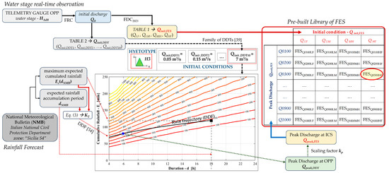
Figure 5.
Flowchart of the proposed Early Warning System [39].
The expected FES is extracted from the pre-built library as a function of the paired Qinit,FES–Qpeak,FES discharge values and is identified by a code made of 7 characters, where the first 5 refer to Qpeak,FES (i.e., Q0100, Q0150, …, Q1000) and the remaining to the initial condition determined by Qinit,FES (i.e., LF, LM, MH, HF); for instance, the FES named Q0500MH refers to the FES obtained considering the design hydrograph with Qpeak,FES equal to 500 m3/s under the low–medium initial discharge class of Qinit,FES (Table 1).
Through the OPP station, it is possible to retrieve the water stage at the time of the EWS evaluation (HAdB) and estimate the corresponding discharge (Q0) using the FRC. Based on Q0, it is then possible to retrieve the nearest values among the ten Qinit,DDT values considered in [39] and reported in Table 1, thus deriving the initial discharge class among the four possible reported in Table 1 (QLF, QLM, QMH, and QHF).
Rainfall forecasts are given by the QPF provided by the National Meteorological Bulletins (NMBs), based on a Sicily LAM. NMBs are issued by the Italian National Civil Protection Department for specific zones every day at 12:00 (Palermo belongs to the zone named “Sicilia S4”). An NMB reports a range of expected cumulative rainfall depth over prefixed accumulation periods of 3, 6, 12, and 24 h. The rainfall forecast refers to a 36 h temporal horizon, from 12:00 of the day of issuing of the bulletin until midnight of the following day. The NMB also provides the possible occurrence (or non-occurrence) of rainfall within regular time windows of 6 h over the forecast period. However, the NMBs do not provide any detailed information about the temporal evolution of the rainfall event, and thus, it is not possible to derive information about the expected hyetograph type.
The value of Qpeak,FES is derived from the QPF and the DDTs described in Section 2.2. More specifically, given the impossibility of deriving predictions about the hyetograph shape from the NMB and adopting a prudential criterion, the EWS refers exclusively to the families of curves relative to the H1 type, which is the hyetograph that generates the maximum flow peak in the case study at equal rainfall volume [39].
The reference family of iso-critical discharge DDT curves at the time of the EWS evaluation is identified exclusively based on the Qinit,DDT value. The following step consists of the computation of a rainfall trajectory based on the QPF from the bulletins, which identifies a curve within the Ec-d plane crossing different iso-critical discharge curves (Figure 5). In particular, the rainfall trajectory is given by the DDF curve passing for the point with the maximum expected cumulated rainfall (Ec in mm) and accumulation period (dNMB in h) indicated in the bulletin. Thus, a couple of values retrieved from the NMB (i.e., Ec and dNMB) are used to determine the return period of the expected rainfall, which is assumed to have critical depth with that return period for any possible sub-duration. The DDF is estimated using the regional rainfall growth curves derived by [54] for the homogeneous subzone of Sicily (i.e., zone S4), including the city of Palermo, characterized by the site-specific couple of parameters a24 = 70.84 and n = 0.36. The rainfall trajectory is generated for a range of duration di varying from 4 h (i.e., minimum duration for the EWS activation) to dNMB as
where the regional growth curve factor KT is obtained by the same Equation (3) considering both the cumulated rainfall E(dNMB) = Ec and duration di = dNMB from the NMB.
E(di) = KT a24 (di/24)n
The parameter associated with the highest iso-critical discharge curves crossing the rainfall trajectory is then identified and is assumed as representative of the highest expected discharge at the OPP section in response to the forecasted rainfall event (Qpeak,OPP). This value is finally incremented by a scaling factor, kp, (discussed in Section 2.5), to take into account the fact that the ICS is downstream the OPP section and finally rounded up to the closest hydrograph peak flow considered for the generation of the FES library in order to determine the corresponding Qpeak,FES; this last, combined with the previously obtained value for Qinit,FES, makes it possible to identify the expected FES from the library.
2.5. Generation of the Pre-Built Library of FESs
The library supporting the EWS includes several FESs that were generated through the following steps:
- Hydrological study aimed to (i) derive six representative hydrographs at the ICS with different return periods (i.e., 10, 25, 50, 100, 300, and 500 years) and (ii) evaluate the scaling factor, kp, between the peak flow at the ICS and the OPP section;
- Normalization of the obtained hydrographs and estimation of a standard Unit Hydrograph (UH);
- Scaling procedure application to the standard UH in order to obtain a set of 19 design hydrographs with peak flow (Qpeak,FES) varying from 100 to 1000 m3/s with steps of 50 m3/s;
- Hydraulic modelling to simulate the propagation of the 19 hydrographs within the computational domain under the four alternative initial conditions defined in Table 1 (i.e., QLF, QLM, QMH, and QHF);
- Derivation of the FES products defined in Section 2.3 (Figure 4) from each simulation;
- Generation of the FES library, where a label, given by paired Qinit,FES and Qpeak,FES values, is associated with each of the 76 generated scenarios (19 Qpeak,FES × 4 Qinit,FES).
2.5.1. Generation of the Design Hydrographs
The hydrological study was carried out using the HEC-HMS [27], which includes a suite of conceptual models that allows for simulating the rainfall–runoff process of a basin. The modelling chain consists of three main components: (1) computation of synthetic hyetographs for a given return period; (2) application of a loss method to derive effective hyetographs; and (3) application of a transform method to derive hydrographs.
The reference area for the hydrological study is the entire drainage area contributing to the runoff generation at the input section (ICS) of the reference computational urban domain for the EWS. It is then constituted by sub-basins SB1 and SB2 (Figure 1). The main characteristics of the two sub-basins are summarized in Table 2. In particular, the SB1, with an extension of approximately 85 km2, has a concentration time of 4 h, while the SB2, with an extension of 29 km2, has a concentration time of 3 h; for both, the concentration times were calculated by the distributed kinematic method.
Table 2.
Main features of sub-basins SB1 and SB2. Tc is the concentration time in h, while CNII and CNIII are the mean areal curve number (SCS-CN method) under the AMC class II (i.e., average moisture condition) and III (i.e., wet moisture condition), respectively.
The rain hyetographs for the six different return periods were generated from the DDFs (Figure 6a) obtained through the regional formulation of [54] and using the Chicago method with centred peak. The highest concentration time between the two sub-basins (i.e., 4 h) was considered critical duration for the rainfall event; this is also consistent with the choice of 4 h as the minimum rainfall duration for the activation of the EWS.
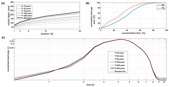
Figure 6.
(a) Depth–Duration–Frequency curves for the 5 considered return periods (i.e., 10, 25, 50, 100, 300, and 500 years); (b) Iso-concentration time curves for the sub-basins SB1 and SB2; (c) Normalized hydrographs for the 5 different return periods and derived standard UH at the ICS (red curve). For helping visualization, this last is reported on logarithmic axes.
The selected loss model for the determination of actual rainfall was the Soil Conservation Service Curve Number (CN) method [55], adopting a prudential criterion by assuming an Antecedent Moisture Condition (AMC) representative of wet conditions (AMC III). Through a geospatial analysis of the most updated (i.e., last update: 2024) version of the Regional Map of the CN available for Sicily, the mean areal values of CNII (i.e., referring to the “average” moisture class, AMC II) were determined for both the sub-basins and then converted into CNIII (i.e., referring to the AMC III), using the specific relationship of the SCS-CN model (Table 2).
The hydrograph for each return period was estimated in HEC-HMS using the User-Specified S-Graph Method, which requires the time–area curve of each sub-basin (Figure 6b), with consideration of temporal discretization of half hour for the precipitation.
For each return period, the obtained hydrograph at the ICS was normalized with respect to its peak flow (Figure 6c). Given that no significant differences were observed among the various normalized hydrographs with reference to a wide range of return periods (i.e., from 10 to 500 years), it was assumed that an acceptable approximation of the normalized hydrograph at the ICS for any return period can be achieved by averaging the 6 normalized hydrographs and deriving a unique standard UH, represented by the red curve in Figure 6c.
The outcomes of the hydrological study were also exploited to explore the relationship between the generic peak flow at the ICS (Qpeak,ICS) and the corresponding peak flow at the upstream section OPP (Qpeak,OPP), which drains only a large portion of the SB1 (Figure 1a). In particular, based on the six simulations with different return periods, this relationship can be well approximated (R2 = 0.98) by a linear regression model with coefficient of 1.33. This value is used as scaling factor, ks, to convert the expected peak flow at the OPP (Qpeak,OPP), obtained according to the procedure described in Section 2.4, into the associated expected peak flow at the ICS (i.e., Qpeak,ICS = ks ∙ Qpeak,OPP), corresponding to the Qpeak,FES of the expected FES.
For the generation of the FES library, we generated a total of 19 design hydrographs, imposing a peak flow value (Qpeak,FES) ranging from 100 m3/s (i.e., corresponding to the peak discharge of the hydrograph with a return period of about 10 years) to 1000 m3/s (i.e., approximately corresponding to the peak discharge of the hydrograph with a return period of 500 years), with a step of 50 m3/s. Each design hydrograph is obtained by multiplying the standard UH (Figure 6c) by the imposed peak flow. The lowest Qpeak,FES selected can be considered the value corresponding to the first event generating CPs within the domain, while the highest is a value over which the number of CPs does not increase, although the water levels, the velocities, and the extension of the flooded areas continue to increase. The step of discretization for Qpeak,FES represents a trade-off solution aimed at reducing the computational effort for creating the library and, at the same time, adequately characterizing the different responses of the basin to different rainfall events.
2.5.2. Hydraulic Modelling
The FESs were obtained by simulating in HEC-RAS [28] the propagation of each design hydrograph within the hydraulic domain and under different initial conditions, according to the approach described in Section 2.3. The HEC-RAS allows for solving De Saint Venant’s shallow water equations by a numerical approach using the finite volume method, simulating the temporal behaviour of water levels and velocities at all nodes of the computational domain. The spatial discretization of the area is based on a polygonal mesh with cells of different shapes, in the centres of which the values of water level and velocity are determined.
The domain is predominantly subject to two-dimensional propagation phenomena; therefore, 2D hydraulic simulations were performed under unsteady flow conditions, for which it was necessary to define (1) the terrain morphology model; (2) the computational mesh; (3) the structural elements affecting flow direction (e.g., walls, river embankments, roads); (4) the spatial variability of Manning’s coefficient across the domain; (5) the boundary conditions; and (6) the parameters of the calculation runs. The HEC-RAS version used in this study (i.e., v.6.4.1) allows for inserting river crossing structures (e.g., bridges and culverts) in the 2D domain, accounting for their geometry and computing energy losses that occur in reaches immediately downstream and upstream of the structure and at the structure itself.
Besides the computational domain definition, which was already discussed in Section 2.1.2, it was necessary to define the initial conditions of simulations along with two boundary conditions of the domain: (i) the upstream condition for incoming flow (i.e., the design hydrograph at the ICS associated with each FES and used to force the model); (ii) the downstream condition for outgoing flow (i.e., transition to the Normal Depth was imposed at the outlet section). The initial conditions are provided by always imposing a null initial water stage for the entire calculation domain and assuming one of the four possible characteristic values of the discharge classes reported in Table 1. These values (i.e., QLF, QLM, QMH, and QHF in Table 1), referring to the OPP section, were rescaled by using the scaling factor, ks, thus obtaining the corresponding discharge values at the ICS, which were used as initial conditions for the hydraulic simulations.
3. Results
3.1. Analysis of the Critical Flooding Points
The hydraulic simulations provide, for each tested scenario, the evolution in time of the flooded areas and the water depth and velocity across the reference domain for the EWS; this allows for determining the location (CPloc) and timing (CPtime) of critical flooding points (CPs) for any FES. In particular, the onset time of a critical flooding point, CPtime, is computed starting from the beginning of the design rainfall event for the considered scenario. The number of CPs and their onset times can vary with the FES; specifically, the number of CPs tends to increase progressively, moving from scenarios with lower hydrograph peaks to those with higher peaks, although different FESs show critical points at the same location. From the analysis of the most severe FES (i.e., Q1000HF), it is then possible to visualize the location (CPloc) of all potential critical points in the study area and assign them an ID code; in particular, the CPs were progressively numbered based on their insurgence time under the FES Q1000HF (Figure 7a). Less severe FESs, such as the Q0300LF (shown in Figure 7b), display only a subset of the CPs of the Q1000HF, which are characterized by different and shorter onset times. The chronological order of the insurgence times of the various CPs could vary with FES with respect to what resulted under the FES Q1000HF, even if this occurred sporadically; thus, for FESs different from the Q1000HF, a CP with a given ID could occur before one identified by a lower ID code.
Figure 7.
(a) Flood map for the most severe FES, i.e., the Q1000HF (Qpeak,FES = 1000 m3/s, Qinit,FES = QHF), with identification of the 34 occurring CPs. (b) flood map for the FES Q0300LF (Qpeak,FES = 300 m3/s, Qinit,FES = QLF), with identification of the 24 occurring CPs (these are identified by the same ID codes relative to the FES Q1000HF).
The knowledge of the number, location, and timing of the expected CPs is a fundamental and strategic aspect of planning and activating efficacious mitigation measures as a function of the expected flood scenario and consequentially reducing the hydraulic risk associated with that event. In the following, an analysis performed for the FESs obtained under Qinit,FES = QHF is presnted. Figure 8 shows a comparison between the different FESs in terms of onset times (in h) at the various CPloc; each segment is relative to a specific CP and shows the lowest onset time on the left limit, which occurs at all CPs for the most severe scenario (i.e., Q1000HF), and the highest onset time on the right limit, with an indication of the corresponding FES. From the figure, it is possible to observe that for most of the FESs, the river begins to flood at the various CPs before the peak time of the design hydrograph (i.e., constant for all FESs and equal to 4 h). For all FESs in the library, floods occur rapidly at the first four CPs (i.e., always in less than 3 h after rainfall onset, with a minimum of 1.5 h), which are also the only critical flooding points occurring for the least severe scenario (i.e., Q0100HF); this would suggest planning some permanent and/or structural measures at those locations, such as a new arrangement of the embankments.
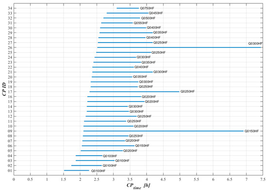
Figure 8.
Onset times of the CPs with respect to the rainfall onset time (CPtime) for FESs obtained with Qinit,FES = QHF. Each segment refers to a specific CP, whose location is reported in Figure 7a, and reports the variation range of CPtime among the various FESs. The left limit of each segment denotes the minimum CPtime, which always occurs for the FES Q1000HF. On the right limit of each segment the maximum CPtime is reported, also indicating the corresponding Qpeak,FES (i.e., from Q0100 to Q0950).
Passing from the FESs Q0100HF to the Q0400HF, the number of CPs increases rapidly up to 30 points, all having onset times ranging approximately between 2 and 4 h, except for the CPs with ID09, ID17, and ID26 that show CPtime over 5 h for the FESs Q0150HF, Q0250HF, and Q0300HF, respectively. Considering the relatively low water levels and velocities for these scenarios, the overall preannouncement time, given by the CPtime plus the forecasting time of the NMB, could allow for activating some temporary mitigation measures there, such as temporary floodproofing barriers.
The four remaining CPs (i.e., from ID31 to ID34) occur as last critical points of flooding only for extreme and relatively rare scenarios with peak flow over 450 m3/s, showing CPtime always between 2.6 and 4.1 h. Under these severe FESs, about half of the CPs occur no later than 2.5 h after the rain onset. To reduce the risks associated with these critical scenarios, more impactful measures should be planned. For instance, in the context of non-structural mitigation strategies, the EWS could recommend temporarily closing certain streets to pedestrian and vehicular traffic, evacuating specific buildings, or even entire districts of the city.
Analogous analyses on the FESs obtained under different initial conditions (i.e., QLF, QLM, QMH), not shown here, highlighted a behaviour very similar to that observed for QHF in terms of the number and displacement of CPs across the study area at equal Qpeak,FES, while a slight and increasing delay can be noticed for any CP when Qinit,FES decreases. The difference in the CPtime between FESs computed under QLF and QHF at equal Qpeak,FES, resulted in being, on average, equal to only 0.3 h.
The outcomes from the analysis of the critical flooding points then indicate that the expected hydrograph peak flow significantly affects the location and timing of flooding. On the other hand, the consideration of different initial conditions (i.e., Qinit,FES), at least in the range from QLF to QHF herein explored, has a much lower effect on the CPs, mainly noticeable in the onset times, especially for the least severe scenarios.
3.2. Floodable Areas and Hazard Variability across Different FESs
Each FES includes various products that allow for a comprehensive assessment of the potential implications related to different flooding events potentially affecting the study area. This makes the EWS a highly effective decision support tool for selecting preventive measures to alert the population and protect the most vulnerable areas of the city. The FES Q1000HF is the worst-case scenario present in the library; beyond the map of the flood extent already shown in Figure 7a, it includes the hazard map for people (Figure 9a), vehicles (Figure 9b), and buildings (Figure 9c), generated according to the criteria discussed in Section 2.3. It is worth emphasizing that the classification of the hazard rate for vehicles and buildings is limited to two specific sub-domains (Figure 1c,d), including the streets and a 3 m buffer zone around each building, respectively. This is emphasized in the inset boxes of Figure 9b,c, specially added for this study to help the map visualization and not provided as FES products.
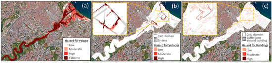
Figure 9.
Flood Event Scenario FES1000HF—hazard maps for (a) people; (b) vehicles; (c) buildings. Inset boxes in Figure 9b,c show a zoom for specific areas to help visualization, and they are not included as final products of the FESs.
Figure 9a presents how under the most catastrophic event considered for FES library generation, the hazard for human stability and people would interest a large portion of the calculation domain (i.e., 45.8%, almost coincident with the flooded portion of the domain), with “high” (mainly around the river’s outlet) or “extreme” (mainly along the river) hazard in the 89.5% of the area with not null hazard. The hazard for vehicles (Figure 9b) would interest almost 30% of the areas covered by streets within the domain, with a hazard ranging from “moderate” to “high” in 80.7% of them, mainly localized in the river’s outlet zone. The areas classified with not null hazard for buildings are the 42% of the considered sub-domain (Figure 9c), even if over 92% of them are classified with a “low” or “moderate” hazard rate, which implies that only partial damage could occur in the buildings located there.
An overview of the complete library reveals that, in agreement with the previous analysis on the CPs, the consequences of the flood events rapidly intensify with increasing Qpeak,FES up to 450 m3/s, while the extent of the flood areas and the associated hazards for FESs grow less rapidly for higher Qpeak,FES. For instance, Figure 10 presents an analysis, again conducted only on all FESs derived under Qinit,FES = QHF, highlighting the variability with Qpeak,FES of the percentage coverage of the domain for each class arising from the flood maps (Figure 10a) and the hazard maps for people (Figure 10b), vehicles (Figure 10c), and buildings (Figure 10d). For Figure 10c,d, the percentages are computed with respect to the specific sub-domains for vehicles and buildings, respectively. From the figure, it can be noticed that all the various hazard classes progressively increase with the expansion of the flooded areas up to Qpeak,FES = 400 m3/s (500 m3/s for the hazard maps for vehicles). Beyond this point, the increase in new areas potentially affected by hazards is less rapid, and the areas already classified with the lowest hazard rate tend to intensify their hazard class, transitioning from the “low” or “moderate” to “high” or “extreme” classes. This explains why, in Figure 10a,b, after the point corresponding to Qpeak,FES = 400 m3/s, there is an overall reduction in the percentage of areas classified as “low”, “moderate”, and “high” with increasing Qpeak,FES, accompanied by an increase in the percentage of areas classified as “extreme”. Analogous analyses on the FESs generated under different Qinit,FES (not shown here) revealed the same trends shown in Figure 10 and highlighted insignificant differences in the percentage coverage of the various classes for all the maps of FESs with equal Qpeak,FES and different Qinit,FES; this confirms that the different initial river flow conditions considered for the FESs generation mainly influence the onset times of floods rather than their extension and magnitude, especially for the most severe FESs.
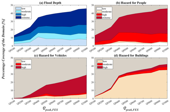
Figure 10.
Flood Event Scenarios derived for Qinit,FES = QHF. Variation in the percentage coverage of the domain of each class for the (a) flood map and the hazard maps for (b) people, (c) vehicles, and (d) buildings as a function of the expected Qpeak,FES.
3.3. Testing the EWS with a Historical Event
The last flooding event of the Oreto River occurred during the night of 3 November 2018 (onset time approximatively at 21:00), and it is herein used as a testing event (TE) for the EWS; actually, this was the only significant fluvial flood interesting the study area since the telemetry hydrometric station installation at the OPP, and, consequentially, the only suitable event for testing the proposed approach on a real case.
The TE occurred with moderate severity, particularly interesting the urban district of Fondo Picone (Figure 11) within an area of the domain where four potential CPs are located (i.e., CP ID06, 07, 09, and 15). Relatively moderate water levels and flow velocities have fortunately caused limited damages, thanks in part to the low traffic on the roads within the flooded areas during nighttime. Minor floodings may have also occurred in other areas of Palermo adjacent to the riverbanks, even if no damage to buildings or people was reported by the Civil Protection Service (SPC) of Palermo for zones different from Fondo Picone. According to the reconstruction operated by the SPC (blue shaded area in Figure 11a), the flooding was due to the overflow of the left embankment of the Oreto River, visible in Figure 11d, without any breach. It reached an extent of about 1.54 ha with estimated maximum water depths averaging around 70 cm and slightly exceeding 1 m in proximity to the river. Actually, considering the reported damages after the event and other information retrieved online and from newspapers, the flood also extended over the areas around via Fondo Picone external to area reported by the SPC, interesting a larger area of about 2.96 ha, delineated by the dashed magenta line in the inset plot of Figure 11a; this is also consistent with the pictures of via Fondo Picone reported in Figure 11b,c,e, also confirming the estimated water depths. No other relevant information emerged from the comparison of the Planet Scope satellite images taken at 9.25 a.m. on 3 November (pre-event) and the 4th (post-event), probably due to the moderate magnitude of the flooding and the time lag in the acquisition of the post-event image.

Figure 11.
(a) Flood map reconstructed by the SPC with the red inset plot showing the reconstruction of the actual flooded area from Google Map Satellite. Post-event pictures from the web portal of the online newspapers Palermo Today (www.palermotoday.it, accessed on 9 November 2018), reported in figures (b,c), and Giornale di Sicilia (www.gds.it, accessed on 11 November 2018), reported in figures (d,e). Their localization in the inset of Figure 11a is denoted by using boxes of different colours associated with the contour line of each picture.
The critical rainfall event causing the TE is herein reconstructed through the analysis of the high-resolution data collected at the Palermo rain gauge managed by the SIAS Regional Agency (Servizio Informativo Agrometeorologico Siciliano), whose location is reported in Figure 1a. Figure 12a shows the rainfall recorded during the forecasting horizon of the bulletins issued on Nov. 2nd (NMB1) and the following day (NMB2), both covering the TE time. The rainfall event started around 14:30 on 2 November and ended at 21:10 of the following day, carrying a total cumulative rainfall of 73.2 mm, with 72.2 mm in about 15 h, starting from 05:50 of 3 November; 79% of this last amount (i.e., 57 mm) was concentrated in only 4 h between 16:20 and 20.20.
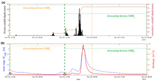
Figure 12.
(a) Rainfall hyetograph (black bar, left y-axis) recorded at the Palermo–SIAS rain gauge and cumulative rainfall depth (purple dashed line, right y-axis) during the time window covering the forecasting horizons for NMB1 and NMB2. (b) Temporal trace of water stages recorded at the OPP (dashed blue line, left y-axis) and corresponding hydrograph (red line, right y-axis) obtained by Equation (1), with indication of the initial discharge at the time of issuing of the two bulletins (black circles). Times of issuing and the forecasting horizons of each bulletin are highlighted in both graphs (in orange for NMB1 and in green for NMB2).
The period antecedent of the TE was extremely rainy, with a total monthly rainfall in October, measured at the same SIAS gauge, equal to 201 mm plus 80 mm, almost equally distributed in the first two days of November, which led to very wet initial moisture conditions. This was also reflected in the temporal trace of the water stages at the OPP, reported in Figure 12b (left y-axis), together with the associated discharge hydrograph (right y-axis), derived using the FRC (Equation (1)). As can be seen in the figure, the hydrograph reached a peak at the OPP of 117 m3/s at 20:10 on 3 November.
As synthetized in Table 3, considering the QPF of NMB1 and NMB2, the EWS would have been activated for both the bulletins, considering rainfall trajectories derived from the DDF curves characterized by Kt equal to 1.84 and 1.18, respectively, according to Equation (3). Given the water stages recorded at the OPP at the issuing time of the bulletins, for both cases, the EWS would have selected FESs associated with high flow initial conditions (QHF) from the library, and families of DDT curves associated with Qinit,DDT10 and Qinit,DDT09 for NMB1 and NMB2, respectively. The Qpeak,DDT at OPP for NMB1 and NMB2, obtained by combining the expected rainfall trajectories with the selected DDT curves, would have been 288 and 125 m3/s, respectively (Figure 13). These last values, incremented by the scaling factor ks (defined in Section 2.5.1) and rounded up, would have provided at the ICS Qpeak,FES values equal to 400 m3/s and 200 m3/s for NMB1 and NMB2, respectively; thus, the expected FES based on the NMB1 would have been the Q0400HF, while a less severe FES would have been predicted based on the NMB2 (i.e., Q0200HF).
Table 3.
Rainfall forecast according to the NMB1 and NMB2, record data at the OPP station, and variables and parameters computed by the EWS at the time of issuing of the two bulletins. On the last row, the FESs retrieved by the EWS from the library are highlighted in bold.
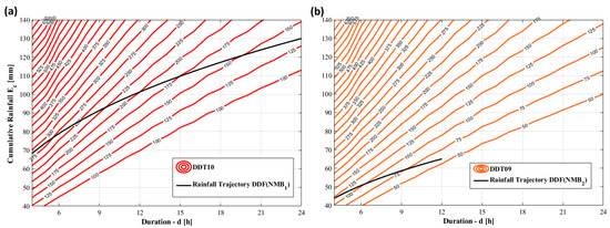
Figure 13.
Family of DDT curves and DDF curves (black curves, providing the expected rainfall trajectory) selected by the EWS for (a) NMB1 and (b) NMB2. For each plot, the coloured lines (red and orange curves) and the associated label indicate the iso-critical discharge DDTs and the corresponding parameter. From the combined use of the two types of curve, the EWS has estimated a Qpeak,DDT equal to 288 m3/s and 125 m3/s for NMB1 and NMB2, respectively, given by the highest DDT crossed by the rainfall trajectory in each plot.
The actual time from the issuing of the bulletin to the onset time of the TE would have been in the order of 33 h and 9 h for NMB1 and NMB2, respectively. As it emerges from the comparison between the values reported in Table 3 and in Figure 12, the maximum QPF predicted by the NMB1 is more than double the value recorded at the Palermo–SIAS rainfall gauge. NMB1, in fact, predicted a cumulative rainfall between 70 and 130 mm in 24 h, with timing coincident with the entire day of 3 November, resulting then consistent with what happened, even if extremely prudential. The following bulletin NMB2 forecasted a range of rainfall from 30 to 65 mm in 12 h, starting at the time of issuing of the same bulletin; in this case, the forecast resulted again consistent with what happened in terms of both total cumulative depth and timing, with a maximum rainfall forecast perfectly aligned with the rainfall recorded. The peak discharge estimated at the OPP by the EWS (Table 3 and Figure 13) would consequently have been much closer to that recorded (Figure 12b) for NMB2 than for NMB1, with percent differences in the order of 146% and 7% for NMB1 and NMB2, respectively. However, it is important to point out that an EWS is always designed according to a cautionary criterium that must consider the uncertainty in the rainfall forecast; an exact reproduction by the EWS of the scenario that occurred was, therefore, not expected, especially for forecasts with longer preannouncement times.
In Figure 14, the flood maps of the FES Q0400HF (i.e., expected FES based on NMB1, Figure 14a) and Q0200HF (i.e., expected FES based on NMB2, Figure 14b) are reported. In the inset graph of each figure, their comparison with the reconstructed flooded area of Fondo Picone (Figure 11a) is also reported. For both cases, the extent of flooding predicted by the EWS fully covers the actual flooded area. The prevision of the EWS based on NMB1 (Figure 14a) results was a little too prudent compared to what actually happened. In particular, due to the considered rainfall that was almost two times that which really occurred in terms of total depth, the EWS would have overestimated the severity of the event, leading to a FES (Q0400HF) that would erroneously have predicted water depths prevalently over 2 m in the test area of Fondo Picone, significant flooding downstream of that area, and the potential triggering of a total of 30 critical flooding points along the right bank of the river, also affecting the right side of the river. The flood dynamic according to the scenario associated with the FES Q0200HF, which the EWS would have provided based on NMB2 (Figure 14b), is extremely close to the characteristics of TE, providing a more accurate estimation of the flooding extent and water depths in the test area (mainly comprised between 1 and 2 m). According to that FES, a total of 11 CPs would have occurred. More specifically, there would have been 5 CPs (i.e., from ID01 to ID05) approximately 1 h before the onset of the 4 CPs within the test area, interesting very small areas near the left bank of the river, consistent with what was observed. Moreover, the CPs ID10 and ID16 would have occurred about 20 min after the onset time of flooding in the test area, with this last affecting a relatively wide downstream zone with low water depths (<0.5 m). No evidence of flooding in this zone has been reported, and it is likely that if flooding did occur, it would have been promptly drained by the urban drainage system.
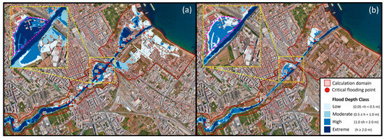
Figure 14.
Flood maps of the FESs Q0400HF (a) and Q0200HF (b), resulting from the application of the EWS based on the NMB1 (bulletin of 2 November 2018) and NMB2 (bulletin of 3 November 2018), respectively. A comparison of both maps with the actual flooded area (dashed magenta contour) in the district of Fondo Picone is reported in the insets.
The EWS would have predicted, in the test area, a predominantly “high” hazard level for human stability for the FES Q0200HF and “extreme” for FES Q0400HF. Regarding the stability of vehicles, they would have provided a prevalent “low” and “extreme” hazard only along the street via Fondo Picone for FES Q0200HF and Q0400HF, respectively. At the same time, the few buildings located around the same street would have been mainly classified with a “low” hazard rate in both FESs. These predictions, especially for the FES Q0200HF, adhere to the fact that only moderate damage related to water infiltration in parked vehicles and some ground-floor apartments has been reported after the flood.
4. Discussion
The proposed EWS for fluvial flood is designed to fully exploit the type of information and instruments available for the study area and minimize the time required to issue alerts. Real-time observations of the water stage at an upstream section of the river and QPF provided by the National Surveillance Meteorological Bulletins (NMBs) have been selected as potential precursors. The former serves as a reliable proxy measure of the overall humidity condition in basins characterized by pluvial regimes, such as the Oreto River basin, where discharges are closely dependent on prior rainfall and antecedent soil moisture in the drainage areas. Alternative approaches, such as those proposed in [56] or those utilizing satellite and/or in situ soil moisture observations, should be considered for systems related to rivers with nival/glacial or ephemeral flow regimes, where discharge may not represent antecedent catchment wetness.
Rainfall forecasting is a key component of any EWS for floods. As demonstrated by the test in Section 3.3, the reliability of the EWS predictions strongly depends on the accuracy of the rainfall forecast. The use of the NMBs offers a good compromise between the forecast accuracy and the potential preannouncement time. The daily frequency of the NMBs and their 36 h temporal forecast horizon ensure a 12 h overlapping window covered by two consecutive NMBs each day. In some cases, such as the one tested here, this overlap can further refine an earlier EWS prediction. For instance, concerning the testing event of this study, the EWS based on NMB1 would have allowed for issuing a warning in a flood-prone area with a long preannouncement time. This would enable civil protection and emergency systems to be alerted and activities to be efficiently prepared (e.g., pre-positioning equipment, supplies, and personnel strategically). Refinement using the following bulletin (NMB2), the last before the event, would have provided a very accurate FES, even if with a shorter preannouncement time (i.e., 9 h), which is still sufficient to implement some protection and/or emergency strategies.
A possible future enhancement of the system could involve incorporating a framework predicting the hyetograph shape from the NMB, for example, considering the information, herein neglected, that distinguishes between “impulsive” and “not impulsive” expected rainfall events, which could be associated with “convective” and “non-convective” events, respectively. Forecasts on the hyetograph shape would allow for fully exploiting the DDTs derived in [39], using all 30 families of iso-critical discharge curves rather than only the 10 considered in this study, thus considerably expanding the FES library.
It is worth emphasizing that, at this early development stage of the proposed EWS, the library includes only FESs generated under the assumption of an unaltered computational domain, neglecting any possible impact that floods may have on altering structures and flood dynamics (e.g., breakage of embankments, collapse of bridges, displacement of large objects induced by high flow, reductions in flow openings due to debris accumulation). Nevertheless, in the future, it would be possible to easily expand the current library with additional scenarios accounting for these negative impacts as well as considering the effects of some protection measures, such as the placement of temporary or permanent floodproofing barriers at critical points.
Moreover, an overview of all FESs in the library could allow for identifying the most susceptible and vulnerable areas in a city, defining potential hazards and risks, and analysing, as performed in Section 3.1 and Section 3.2, the most suitable countermeasures in a cost-benefit framework while considering the city’s peculiarities.
This work primarily focused on non-structural measures for mitigating flood risk. However, an effective and comprehensive flood management strategy in urban areas should combine these measures with structural solutions tailored to the urban context. Such measures might include, for instance, the construction of levees, dikes, and floodwalls; raising embankments along riverbanks, riverbank stabilization, and river widening; repurposing spaces for temporary or permanent floodwater storage (e.g., through detention basins, retention ponds, wetlands, reservoirs, or dams); construction of bypasses, diversion channels, culverts, and stormwater drains; strengthening of existing stormwater management systems; implementation of green spaces; raising of critical infrastructures (e.g., roads, bridges, and utilities) above expected flood levels.
EWS data should inform land use planning, zoning regulations, and building codes to guide future urban development. Policies play a pivotal role in this context. Implementing EWS requires cross-sectoral governance and key policy initiatives that can efficiently lessen the vulnerability of local communities. Governments should mandate the integration of EWS data and technologies into national and local flood management frameworks and update flood preparedness plans. This includes training local officials and communities on interpreting and acting on EWS information. Substantial investment in the infrastructure and technology that support EWSs, such as river monitoring stations, satellite data, and communication systems, is crucial, necessitating government funding allocation for development and maintenance. Policies should also drive public education, awareness campaigns, and community engagement in EWS. This may include the organization of campaigns to educate the public on the necessary actions to take during warnings and the enhancement of community participation in EWS through local committees. Educational programs could lead to changes in public behaviour, making the community more resilient to floods. Finally, policy initiatives might also include social protection and insurance schemes, such as flood insurance and post-disaster financial aid, to mitigate the economic vulnerability of communities.
5. Conclusions
Early Warning Systems (EWS) for fluvial floods are highly suitable and easily implementable non-structural protection measures. They are particularly effective in managing and mitigating the impacts of flooding in urban areas, where the implementation of structural solutions may be hindered by the complex existing urban tissue. Given the growing urbanization and increasing impacts of climate change, the development of this kind of system, even in simple forms like the one proposed here, is becoming increasingly urgent. These systems provide timely and accurate information, enabling authorities and residents to take necessary actions to protect lives and property, and reduce the potential economic losses. Additionally, EWSs facilitate better coordination among various agencies and stakeholders involved in flood management, leading to improved emergency responses and fostering resilient communities.
The EWS proposed in this study can provide the city of Palermo with daily predictions of potential fluvial flood over a 36 h forecast time horizon. Moreover, it could allow for further refinement during the last 12 h of this horizon based on more updated and typically more accurate rainfall forecasts. The computational time is essentially instantaneous since the simulations were previously performed offline during the generation phase of the FES library. This last is easily updateable to account for new urban development processes and expandable to also contemplate other possible scenarios. The products offered by each scenario (i.e., flood map, hazard maps, location and onset time of potential critical flooding points) contain all the essential information needed to assess and localize the potential hazards and activate possible protective actions. For example, in this study, the generation of the FESs’ library has made it possible to identify potential critical flooding points and suggest possible solutions. These include some permanent measures and new arrangements of the embankments, at points particularly susceptible to flooding even for not too severe scenarios, as well as temporary and low-cost mitigation measures, such as floodproofing barriers, whose implementation was suggested at points whose flooding onset time would allow for their activation. Under the most severe scenarios and in areas where other interventions are not practicable, extreme emergency strategies, such as the temporary closure or evacuation of roads, buildings, or entire districts, could be suggested.
The case study discussed here, due to its specific characteristics (e.g., level of urbanization, presence of a river that crosses the city), may serve as a representative example of challenges that many Mediterranean cities may face in the future. Consequently, the proposed EWS could be readily adapted for use in other cities.
Despite its simplicity, the proposed EWS was able to faithfully reproduce a real event, demonstrating a satisfactory ability to issue an alert proportionate to the actual occurrence with a preannouncement time sufficient to activate possible countermeasures. The real flood event considered allowed for testing the EWS in the modality “early prevision and later refinement”, as two consecutive bulletins fully covered the event. This highlighted the key role of rainfall forecasts in the reliability of the EWS predictions. Furthermore, the testing event described in Section 3.3 confirmed the reliability of the different components of the EWS and the results of the simulations for the FES generation.
The EWS should be part of an articulated system that integrates various stakeholders, including communities, authorities, and decision-makers, to achieve risk reduction. This paper mainly focused on the development of some structural components of the EWS, which typically involve the physical infrastructure (e.g., water stage and rain monitoring stations) and technological aspects that enable the generation of timely and meaningful warning information to at-risk communities. Future research directions include the development of non-structural elements, which are effective communication protocols and community engagement to enhance preparedness, prevention, and mitigation efforts. Finally, among the possible future lines of development for the proposed EWS, the possible integration of advanced technologies, such as remote sensing and/or the use of artificial intelligence for predictive analytics, is particularly noteworthy.
Author Contributions
D.P. is the first and corresponding author, and he prepared the original draft. All authors (D.P., M.A., A.F., and L.V.N.) have relevantly contributed to this work, with different and equally important contributions to the conceptualization, methodology, software, validation, formal analysis, investigation, resources, data curation, review and editing, and visualization. All authors have read and agreed to the published version of the manuscript.
Funding
This research did not receive any specific grant from funding agencies in the public, commercial, or not-for-profit sectors.
Data Availability Statement
Most of the data presented in this study are contained within the article. Some of the original data presented in the study are openly available in the repository database cited within the study. Restrictions apply to the availability of water stage records at the OPP and the NMB; data were obtained from AdB and are available with the permission of AdB. The FESs’ Library generated in this study and the included products are available on request from the corresponding author.
Acknowledgments
Thanks to the numerous scientists who provided additional information from their studies. The authors also thank anonymous reviewers for their suggestions on the quality improvement of the present paper.
Conflicts of Interest
The authors declare no conflicts of interest.
References
- European Commission. Datasets, ESM 2015–2019. 2020. Available online: https://ghsl.jrc.ec.europa.eu/esm_R2019.php (accessed on 1 June 2024).
- Noto, L.V.; Cipolla, G.; Francipane, A.; Pumo, D. Climate change in the mediterranean basin (part I): Induced alterations on climate forcings and hydrological processes. Water Resour. Manag. 2023, 37, 2287–2305. [Google Scholar] [CrossRef]
- UN DESA. 2018 Revision of World Urbanization Prospects. UN DESA Publication. 2018. Available online: https://www.un.org/en/desa/2018-revision-world-urbanization-prospects (accessed on 12 June 2024).
- Pumo, D.; Arnone, E.; Francipane, A.; Caracciolo, D.; Noto, L.V. Potential implications of climate change and urbanization on watershed hydrology. J. Hydrol. 2017, 554, 80–99. [Google Scholar] [CrossRef]
- ISPRA. Landslides and Floods in Italy: Hazard and Risk Indicators—Summary Report 2018; Trigila, A., Iadanza, C., Eds.; ISPRA: Rome, Italy, 2018; ISBN 978-88-448-0934-8. Available online: https://www.isprambiente.gov.it/en/publications/reports/landslides-and-floods-in-italy-hazard-and-risk-indicators-2013-summary-report-2018 (accessed on 12 June 2024).
- UNISDR. Towards a Post-2015 Framework for Disaster Risk Reduction. The United Nations Office for Disaster Risk Reduction. 2012. Available online: https://www.undrr.org/publication/towards-post-2015-framework-disaster-risk-reduction (accessed on 12 June 2024).
- Kundzewicz, Z.W. Non-structural Flood Protection and Sustainability. Water Int. 2002, 27, 3–13. [Google Scholar] [CrossRef]
- Acosta-Coll, M.; Ballester-Merelo, F.; Martinez-Peiró, M.; de La Hoz-Franco, E. Real-Time Early Warning System Design for Pluvial Flash Floods-A Review. Sensors 2018, 18, 2255. [Google Scholar] [CrossRef] [PubMed]
- Keil, C.; Craig, G.C. Regime-dependent forecast uncertainty of convective precipitation. Meteorol. Z. 2011, 20, 145–151. [Google Scholar] [CrossRef]
- Silvestro, F.; Rebora, N.; Cummings, G.; Ferraris, L. Experiences of dealing with flash floods using an ensemble hydrological nowcasting chain: Implications of communication, accessibility and distribution of the results. J. Flood Risk Manag. 2017, 10, 446–462. [Google Scholar] [CrossRef]
- Norbiato, D.; Borga, M.; Degli Esposti, S.; Gaume, E.; Anquetin, S. Flash flood warning based on rainfall depth-duration thresholds and soil moisture conditions: An assessment for gauged and ungauged basins. J. Hydrol. 2008, 362, 274–290. [Google Scholar] [CrossRef]
- Zanchetta, A.D.L.; Coulibaly, P. Recent Advances in Real-Time Pluvial Flash Flood Forecasting. Water 2020, 12, 570. [Google Scholar] [CrossRef]
- Alfieri, L.; Salamon, P.; Pappenberger, F.; Wetterhall, F.; Thielen, J. Operational early warning systems for water-related hazards in Europe. Environ. Sci. Policy 2012, 21, 35–49. [Google Scholar] [CrossRef]
- Alfieri, L.; Thielen, J. A European precipitation index for extreme rain-storm and flash flood early warning. Meteorol. Appl. 2015, 22, 3–13. [Google Scholar] [CrossRef]
- Georgakakos, K.P. Analytical results for operational flash flood guidance. J. Hydrol. 2006, 317, 81–103. [Google Scholar] [CrossRef]
- Gourley, J.J.; Erlingis, J.M.; Hong, Y.; Wells, E.B. Evaluation of tools used for monitoring and forecasting flash floods in the United States. Weather Forecast. 2012, 27, 158–173. [Google Scholar] [CrossRef]
- Reed, S.; Schaake, J.; Zhang, Z. A distributed hydrologic model and threshold frequency-based method for flash flood forecasting at ungauged locations. J. Hydrol. 2007, 337, 402–420. [Google Scholar] [CrossRef]
- Javelle, P.; Demargne, J.; Defrance, D.; Pansu, J.; Arnaud, P. Evaluating flash-flood warnings at ungauged locations using post-event surveys: A case study with the AIGA warning system. Hydrol. Sci. J. 2014, 59, 1390–1402. [Google Scholar] [CrossRef]
- Heuvelink, D.; Berenguer, M.; Brauer, C.; Uijlenhoet, R. Hydrological application of radar rainfall nowcasting in The Netherlands. Environ. Int. 2020, 136, 105431. [Google Scholar] [CrossRef] [PubMed]
- Berenguer, M.; Sempere-Torres, D.; Pegram, G.G. SBMcast—An ensemble nowcasting technique to assess the uncertainty in rainfall forecasts by Lagrangian extrapolation. J. Hydrol. 2011, 404, 226–240. [Google Scholar] [CrossRef]
- Vivoni, E.R.; Entekhabi, D.; Bras, R.L.; Ivanov, V.Y.; Van Horne, M.P.; Grassotti, C.; Hoffman, R.N. Extending the predictability of hydrometeorological flood events using radar rainfall nowcasting. J. Hydrometeorol. 2006, 7, 660–677. [Google Scholar] [CrossRef]
- Rebora, N.; Ferraris, L.; von Hardenberg, J.; Provenzale, A. RainFARM: Rainfall downscaling by a Filtered Autoregressive Model. J. Hydrometeorol. 2006, 7, 724–738. [Google Scholar] [CrossRef]
- Silvestro, F.; Rossi, L.; Campo, L.; Parodi, A.; Fiori, E.; Rudari, R.; Ferraris, L. Impact-based flash-flood forecasting system: Sensitivity to high resolution numerical weather prediction systems and soil moisture. J. Hydrol. 2019, 572, 388–402. [Google Scholar] [CrossRef]
- Spyrou, C.; Varlas, G.; Pappa, A.; Mentzafou, A.; Katsafados, P.; Papadopoulos, A.; Anagnostou, M.N.; Kalogiros, J. Implementation of a Nowcasting Hydrometeorological System for Studying Flash Flood Events: The Case of Mandra, Greece. Remote Sens. 2020, 12, 2784. [Google Scholar] [CrossRef]
- Hofmann, J.; Schüttrumpf, H. Risk-Based Early Warning System for Pluvial Flash Floods: Approaches and Foundations. Geosciences 2019, 9, 127. [Google Scholar] [CrossRef]
- Massazza, G.; Tamagnone, P.; Wilcox, C.; Belcore, E.; Pezzoli, A.; Vischel, T.; Panthou, G.; Housseini Ibrahim, M.; Tiepolo, M.; Tarchiani, V.; et al. Flood hazard scenarios of the Sirba river (Niger): Evaluation of the hazard thresholds and flooding areas. Water 2019, 11, 1018. [Google Scholar] [CrossRef]
- US Army Corps of Engineers (USACE). Hydrologic Modeling System HEC-HMS: Technical Reference Manual; Hydrologic Engineering Center: Davis, CA, USA, 2000.
- US Army Corps of Engineers (USACE). HEC-RAS, River Analysis System Hydraulic Reference Manual; Brunner, G.W., Ed.; Hydrologic Engineering Center: Davis, CA, USA, 2016.
- Russo, B.; Gómez, M.; Macchione, F. Pedestrian hazard criteria for flooded urban areas. Nat. Hazards 2013, 69, 251–265. [Google Scholar] [CrossRef]
- Blanco-Vogt, A.; Schanze, J. Assessment of the physical flood susceptibility of buildings on a large scale—Conceptualand methodological frameworks. Nat. Hazards Earth Syst. Sci. 2014, 14, 2105–2117. [Google Scholar] [CrossRef]
- Xia, J.; Falconer, R.A.; Wang, Y.; Xiao, X. New criterion for the stability of a human body in floodwaters. J. Hydraul. Res. 2014, 52, 93–104. [Google Scholar] [CrossRef]
- Xia, J.; Falconer, R.A.; Xiao, X.; Wang, Y. Criterion of vehicle stability in floodwaters based on theoretical and experimental studies. Nat. Hazards J. Int. Soc. Prev. Mitig. Nat. Hazards 2014, 70, 1619–1630. [Google Scholar] [CrossRef]
- Milanesi, L.; Pilotti, M.; Bacchi, R. Using web-based observations to identify thresholds of a person’s stability in a flow. Water Resour. Res. 2016, 52, 7793–7805. [Google Scholar] [CrossRef]
- Martínez-Gomariz, E.; Gómez, M.; Russo, B. Experimental study of the stability of pedestrians exposed to urban pluvial flooding. Nat. Hazards 2016, 82, 1259–1278. [Google Scholar] [CrossRef]
- Martínez-Gomariz, E.; Gómez, M.; Russo, B.; Djordjević, S. A new experiments-based methodology to define the stability threshold for any vehicle exposed to flooding. Urban Water J. 2017, 14, 930–939. [Google Scholar] [CrossRef]
- Chanson, H.; Brown, R. Stability of Individuals during Urban Inundations: What Should We Learn from Field Observations? Geosciences 2018, 8, 341. [Google Scholar] [CrossRef]
- Chen, Q.; Xia, J.; Falconer, R.A.; Guo, P. Further improvement in a criterion for human stability in floodwaters. J. Flood Risk Manag. 2019, 12, e12486. [Google Scholar] [CrossRef]
- Leal, M.; Reis, E.; Pereira, S.; Santos, P.P. Physical vulnerability assessment to flash floods using an indicator-based methodology based on building properties and flow parameters. J. Flood Risk Manag. 2021, 14, e12712. [Google Scholar] [CrossRef]
- Forestieri, A.; Caracciolo, D.; EArnone Noto, L.V. Derivation of Rainfall Thresholds for Flash Flood Warning in a Sicilian Basin Using a Hydrological Model. Procedia Eng. 2016, 154, 818–825. [Google Scholar] [CrossRef]
- INRIX. Inrix 2022 Global Traffic Scorecard. 2022. Available online: https://inrix.com/scorecard (accessed on 12 June 2024).
- Pumo, D.; Viola, F.; La Loggia, G.; Noto, L.V. Annual flow duration curves assessment in ephemeral small basins. J. Hydrol. 2014, 519 Pt A, 258–270. [Google Scholar] [CrossRef]
- Chow, V.T. Open-Channel Hydraulics; McGraw-Hill Book Co.: New York, NY, USA, 1959. [Google Scholar]
- Martina, M.L.V.; Todini ELibralon, A. A Bayesian decision approach to rainfall thresholds based flood warning. Hydrol. Earth Syst. Sci. 2006, 10, 413–426. [Google Scholar] [CrossRef]
- Golian, S.; Saghafian, B.; Maknoon, R. Derivation of probabilistic thresholds of spatially distributed rainfall for flood forecasting. Water Resour. Manag. 2010, 24, 3547–3559. [Google Scholar] [CrossRef]
- Montesarchio, V.; Lombardo, F.; Napolitano, F. Rainfall thresholds and flood warning: An operative case study. Nat. Hazards Earth Syst. Sci. 2009, 9, 135–144. [Google Scholar] [CrossRef]
- Noto, L.V. Exploiting the Topographic Information in a PDM-Based Conceptual Hydrological Model. J. Hydrol. Eng. 2014, 19, 6. [Google Scholar] [CrossRef]
- Radice, A.; Longoni, L.; Papini, M.; Brambilla, D.; Ivanov, V.I. Generation of a Design Flood-Event Scenario for a Mountain River with Intense Sediment Transport. Water 2016, 8, 597. [Google Scholar] [CrossRef]
- Yin, J.; Yu, D.; Yin, Z.; Wang, J.; Xu, S. Modelling the anthropogenic impacts on fluvial flood risks in a coastal mega-city: A scenario-based case study in Shanghai, China. Landsc. Urban Plan. 2015, 136, 144–155. [Google Scholar] [CrossRef]
- Salvati, P.; Petrucci, O.; Rossi, M.; Bianchi, C.; Pasqua, A.A.; Guzzetti, F. Gender, age and circumstances analysis of flood and landslide fatalities in Italy. Sci. Total Environ. 2018, 610, 867–879. [Google Scholar] [CrossRef] [PubMed]
- Wallingford, H.R.; Flood Hazard Research Centre; Middlesex University; Risk & Policy Analysts Ltd. Flood Risks to People, Phase 2, FD2321/TR2 Guidance Document. Defra and UK Environment Agency: Flood and Coastal Defence R&D Programme; Department for Environment, Food and Rural Affairs: London, UK, March 2006; PB NO. 11545. Available online: https://assets.publishing.service.gov.uk/media/602bbc3de90e07055f646148/Flood_risks_to_people_-_Phase_2_Guidance_Document_Technical_report.pdfwww.defra.gov.uk/environ/fcd/research (accessed on 12 June 2024).
- Reiter, P. International Methods of Risk Analysis, Damage Evaluation and Social Impact Studies Concerning Dam-Break Accidents; Technical Report of the EU-Project RESCDAM; Helsinki PR Water Consulting: Seinäjoki, Finland, 2000. [Google Scholar]
- Maijala, T. Rescdam: Development of Rescue Actions Based on Dam-Break FLOOD Analysis; Final Report, Grant Agreement No.650. Subv 99/52623 Community Action Programme in the Field of Civil Protection; Finnish Environment Institute: Helsinki, Finland, 2001; Available online: https://civil-protection-humanitarian-aid.ec.europa.eu/system/files/2014-11/rescdam_rapportfin.pdf (accessed on 12 June 2024).
- Clausen, L.; Clark, P.B. The development of criteria for predicting dam-break food damages using modelling of historical dam failures. In International Conference on River Flood Hydraulics; White, W.R., Ed.; John Wiley & Sons Ltd.: Hoboken, NJ, USA; Hydraulics Research Limited: Wallingford, UK, 1990; pp. 369–380. [Google Scholar]
- Forestieri, A.; Lo Conti, F.; Blenkinsop, S.; Cannarozzo, M.; Fowler, H.J.; Noto, L.V. Regional frequency analysis of extreme rainfall in Sicily (Italy). Int. J. Climatol. 2018, 38, e698–e716. [Google Scholar] [CrossRef]
- SCS. Soil Conservation Service (SCS). Hydrology. In National Engineering Handbook; Soil Conservation Service; USDA: Washington, DC, USA, 1993; Section 4, Chapter 4. [Google Scholar]
- Brocca, L.; Liersch, S.; Melone, F.; Moramarco, T.; Volk, M. Application of a model-based rainfall-runoff database as efficient tool for flood risk management. Hydrol. Earth Syst. Sci. 2013, 17, 3159–3169. [Google Scholar] [CrossRef]
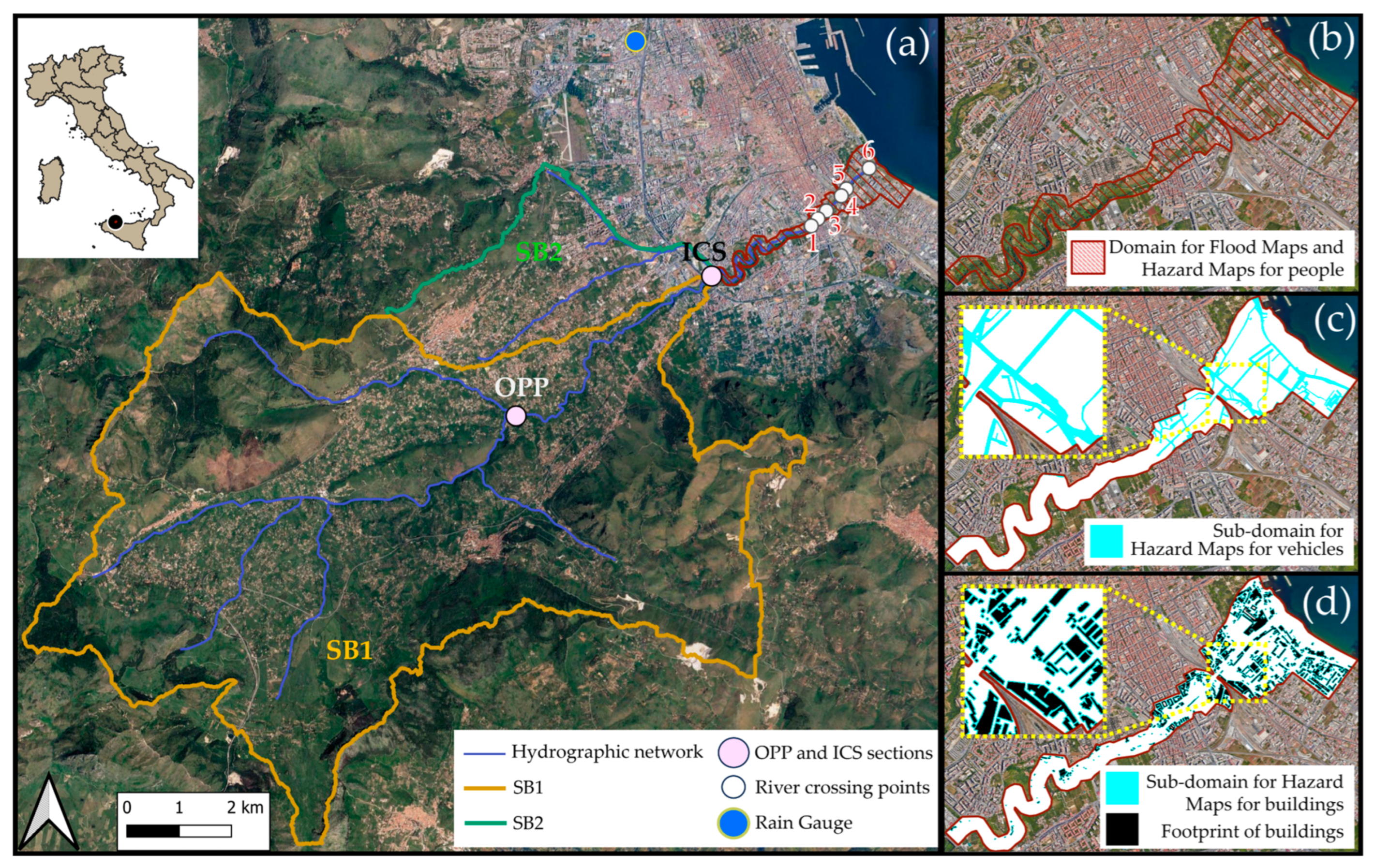


Disclaimer/Publisher’s Note: The statements, opinions and data contained in all publications are solely those of the individual author(s) and contributor(s) and not of MDPI and/or the editor(s). MDPI and/or the editor(s) disclaim responsibility for any injury to people or property resulting from any ideas, methods, instructions or products referred to in the content. |
© 2024 by the authors. Licensee MDPI, Basel, Switzerland. This article is an open access article distributed under the terms and conditions of the Creative Commons Attribution (CC BY) license (https://creativecommons.org/licenses/by/4.0/).