Abstract
The freshwater discharge from catchments along the Gulf of Alaska, termed Alaska discharge, is characterized by significant quantity and variability. Owing to subarctic climate and mountainous topography, the Alaska discharge variations may deliver possible impacts beyond the local hydrology. While short-term and local discharge estimation has been frequently realized, a longer time span and a discussion on cascading impacts remain unexplored in this area. In this study, the Alaska discharge during 1982–2022 is estimated using the Soil and Water Assessment Tool (SWAT). The adequate balance between the model complexity and the functional efficiency of SWAT suits the objective well, and discharge simulation is successfully conducted after customization in melting calculations and careful calibrations. During 1982−2022, the Alaska discharge is estimated to be 14,396 ± 819 m3⋅s−1⋅yr−1, with meltwater contributing approximately 53%. Regarding variation in the Alaska discharge, the interannual change is found to be negatively correlated with sea surface salinity anomalies in the Alaska Stream, while the decadal change positively correlates with the North Pacific Gyre Oscillation, with reasonable time lags in both cases. These new findings provide insights into the relationship between local hydrology and regional climate in this area. More importantly, we provide rare evidence that variation in freshwater discharge may affect properties beyond the local hydrology.
1. Introduction
River discharge from continents to oceans accounts for a global average of 36,055 km3⋅yr−1 [1]. It plays a non-negligible role in the Earth’s hydrological and biogeochemical cycles by delivering freshwater, essential sediments, and nutrients to the ocean [2,3,4]. The quantity of and variation in freshwater discharge are the most crucial parameters among many others [5,6]. Specifically, freshwater discharge can freshen the seawater and deliver impacts on large-scale ocean processes such as thermohaline circulation [7]. For example, a thermohaline circulation existing in the North Pacific Ocean has been shown to significantly influence the local and global climate and marine ecosystems via the redistribution of heat and the transportation of organic carbon and nutrients [8,9,10,11]. The strength of this circulation process is primarily controlled by the sea surface salinity. According to Uehara et al. [12], anomalies in the sea surface salinity may have impacts on the overturning in the northwestern Sea of Okhotsk. These anomalies can propagate along the current pathway from the Alaskan Stream, central Bering Sea, western subarctic gyre, East Kamchatka Current region, and eastern Okhotsk Sea (Figure S1). Following on from this finding, a significant negative correlation was revealed between the interannual variation in sea surface salinity in the northwestern Sea of Okhotsk and the variation in annual river discharge from the Kamchatka Peninsula, which is located upstream of the overturning along the current pathways [13]. Similarly, the role of freshwater discharge from the catchments along the Gulf of Alaska (GOA) (hereafter referred to as the Alaska discharge) was hinted at but has not yet been adequately explored. Therefore, the present study aims to investigate the correlation between the Alaska discharge and sea surface salinity anomalies in the Alaskan Stream, which is an upstream component of the salt pathway. The significant Alaska discharge into the neighboring oceans is a result of rainfall, snow and ice melt, and little human activity in the Alaskan region. Furthermore, variations in the Alaska discharge exhibit sensitivity to atmospheric phenomena over the North Pacific Ocean and to global climate change [14,15,16]. However, the long-term variations in the Alaska discharge and their connection with corresponding atmospheric variability remain little known. One potential factor influencing the hydrological processes in the catchments along the GOA is the North Pacific Oscillation (NPO), a large-scale atmospheric variability observed over the North Pacific Ocean. The NPO is characterized by a seesaw north–south dipole of sea level pressure anomalies between the Aleutian Low and North Pacific High [17,18]. Therefore, a comprehensive estimation of the Alaska discharge and its variation can contribute to a better understanding of the connections between regional discharge, large-scale atmospheric variations, and ocean processes in the North Pacific sector.
Various methods can be used to estimate discharge, including the rating curve method, the velocity-area method, hydrological modeling, and remote sensing techniques [19,20,21,22]. Among these options, hydrological models, which include empirical, conceptual, and process-based models, offer an adaptable approach to simulate the processes of water movement under various land cover and soil conditions [23,24,25]. Several studies on the Alaska discharge have primarily focused on estimating the total volume, analyzing the contributions of hydrological components, and examining seasonal variations by using various hydrological models. For instance, Wang et al. [15] simulated the Alaska discharge and its seasonal and interannual variations by developing a digital elevation model (DEM) that simplifies the main physical processes within the catchment, including rainfall-runoff, snow and ice storage, and melting processes. Neal et al. [26] estimated the annual Alaska discharge and its contribution from glaciers and icefields using a combination of measured discharge and enhanced precipitation models. Similarly, Hill et al. [27] developed regression equations to estimate the monthly Alaska discharge at high resolution based on various physical characteristics of the basin, including the area, mean elevation, and land cover, as well as meteorological characteristics such as temperature and precipitation. Moreover, Beamer et al. [28] estimated the Alaska discharge and examined its source components with good accuracy by using a suite of distributed, process-based models, with consideration of important hydrological processes such as rainfall-runoff, evapotranspiration (ET), infiltration, baseflow runoff, and snow and ice melting.
While these studies confirm that process-based hydrological models provide a comprehensive and efficient representation of real hydrological processes, there are still unresolved questions, particularly regarding the spatial variability of the model parameters. These parameters, which account for different catchment characteristics and climate forcing, are often underrepresented at the basin scale. Additionally, although these studies provide plausible historical discharge estimates (700–900 km3 during 1961–2014), an extensive exploration of recent estimations is necessary to better understand the long-term variations in the Alaska discharge, given the climatic variation. Furthermore, the influence of the Alaska discharge variations on coastal oceanic systems, such as sea surface salinity in the surrounding ocean sector, remains underexplored.
Hence, the present study builds on previous work by focusing on the following: (i) estimating the Alaska discharge during 1982–2022, using a process-based hydrological model, namely, the Soil and Water Assessment Tool (SWAT, [29,30]) with modified melting processes, (ii) investigating spatiotemporal variations in the Alaksa discharge, (iii) exploring the correlations between variations in the Alaska discharge and atmospheric phenomena, as well as sea surface salinity, to provide a more comprehensive understanding of the atmosphere–land–ocean interactions. First, the details of the study area, the SWAT application and its inputs, and the SWAT calibration and validation, as well as the statistical approach for analyzing the discharge, are introduced in Section 2. The model calibration, validation, and simulation results are then presented in Section 3, along with the connection between the Alaska discharge and atmospheric variability. The relationship between the Alaska discharge and the North Pacific Ocean is discussed in Section 4. Finally, the key conclusions are summarized in Section 5.
2. Materials and Methods
2.1. Study Area
The catchments along the GOA (hereafter referred to as the Alaska catchment) span the southern region of Alaska and a portion of Canadian territory (54–64° N, 125–157° W), bordering the GOA in the Northeastern Pacific Ocean (Figure 1a). The present study focuses on the Alaska catchment which covers an area of approximately 320,000 km2, including five major basins, namely the following: the Susitna (44,391 km2), Copper (60,451 km2), Alsek (28,298 km2), Taku (11,013 km2), and Stikine (47,734 km2) basins, in addition to numerous ungauged basins (127,902 km2). The Alaska catchment has a large range of elevation, with an average height of around 1000 m and some peaks over 3000 m (Figure 1b). The region is covered by a number of mountains that contribute to the complex topography. The major mountain ranges that define the basins include the Coast Mountains in the southeast, the Wrangell-St. Elias Mountains in the east, the Chugach Mountains along the central coast, the Alaska Range stretching from east to west in the northern area, and the Kenai Mountains on the Kenai Peninsula. Particularly, the Wrangell-St. Elias Mountains, above 5000 m, are covered by extensive glaciers. Meanwhile, the Chugach Mountains along the central coast block moist Pacific air, leading to high precipitation on the coastal side and drier conditions inland. The Alaska Range, a long (~1000 km) west–east mountain range, includes the highest peak in North America and is characterized by a tough climate and significant glaciation. Due to the rugged topography, the following 5 slope classes were established across all subbasins in the Alaska catchment: 0–3%, 3–15%, 15–30%, 30–60%, and >60%, based on DEM [31] using ArcGIS 10.7.1 software. Most areas (78%) fall within the 3–60% slope range. Additionally, according to North America Land Cover 2015 [32], the study area consists of various land cover types (Table S1), dominated by forest (32.3%), particularly subpolar taiga, polar or subpolar shrubland–lichen–moss (25.5%), barren land (34.1%), glaciers (17.8%), and wetlands (3.48%).
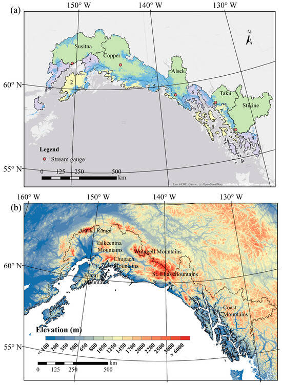
Figure 1.
(a) The Alaska catchment showing the five basins (green) and ungauged basins (purple and yellow), with glacial coverage (blue), along with the streamflow gauging stations (red points). (b) The topography of the Alaska catchment, as obtained from the ASTER Global DEM Version 3.
The climate in the study area is diverse, due to the high latitude, complex topography, and proximity to the ocean [33]. The higher-latitude region is dominated by cold climates that result in long, cold winters and brief, cool summers, with the Alaska Range experiencing a polar climate [34,35]. Meanwhile, the lower-latitude region is characterized by boreal and warm temperate climates, thus leading to humid conditions associated with relatively mild winters and cool summers [33,34,36]. Lader et al. [37] used reanalysis data from 1979 to 2009 to analyze the near-surface air temperature and precipitation for the Alaska region. Their findings indicated that the average monthly temperature during winter is approximately −12 °C, with an average precipitation of around 6 cm, while the temperatures in the Alaska Range drop below −15 °C and the precipitation exceeds 15 cm. Except for parts of the Alaska Range, summer temperatures in the higher-latitude regions are approximately 10 °C, with precipitation ranging between 10–20 cm. Moreover, the southeastern region is the warmest part of the study area during winter, with average temperatures close to freezing, and a monthly average precipitation of above 20 cm. Although no uniform trend in the annual precipitation is observed across the Alaska catchment, a significant increase in the annual temperature is observed between 1957 and 2021, with a rate of roughly 0.4 °C⋅decade−1 [38]. These variable climate conditions potentially influence the hydrological processes across the Alaska catchment.
These important characteristics such as topography and climate directly influence the Alaska discharge quantity and variability. The discharge is predominantly generated in the mountainous areas that receive substantial snow and rain, with the highest discharge rates observed in low-elevation regions covered by large coastal glaciers [28]. Additionally, the phase of precipitation input depends on the air temperature variability, leading to a strong seasonal cycle. The diverse climate of the Alaska catchment, varying from polar in the Alaska Range to temperate in the lower-latitude coastal regions, primarily controls the timing and magnitude of meltwater.
2.2. Model Setup and Configuration
Herein, the SWAT model is used to estimate the discharge during the study period of 1982–2022, as well as the warm-up period during 1979–1981 (methodological flowchart in Figure 2). The SWAT model is a semi-distributed process-based hydrological model that is capable of simulating the water transport in river basins. Specifically, the ArcSWAT 2012 extension (hereafter referred to as SWAT) of the ArcGIS 10.7.1-based graphical interface is used in this study to process the discharge simulation. The SWAT model delineates a basin and divides it into a series of subbasins depending on topography. These subbasins are further divided into the smallest unit, namely the hydrological response unit (HRU), based on the homogeneous type of land cover, soil, and slope. The SWAT model then calculates the water balance at the HRU level, aggregates it at the subbasin level, and finally routes it towards the channels and outlet of the basin [39]. The water balance is calculated using Equation (1) [30]:
where SWt is the final soil water content (mm), SW0 is the initial soil water content (mm) on day 0, t is time (days), Rday is the amount of precipitation (mm) on day i, Qsurf is the amount of surface runoff (mm) on day i, Ea is the amount of evapotranspiration (mm) in day i, Wseep is the amount of water (mm) entering the vadose zone from the soil profile on day i, and Qgw is the amount of groundwater discharge (mm) on day i.
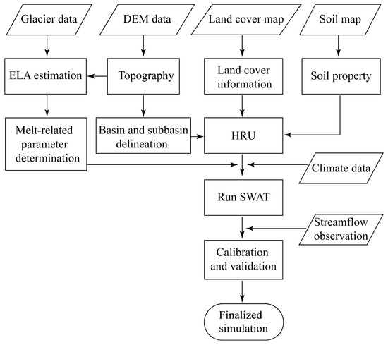
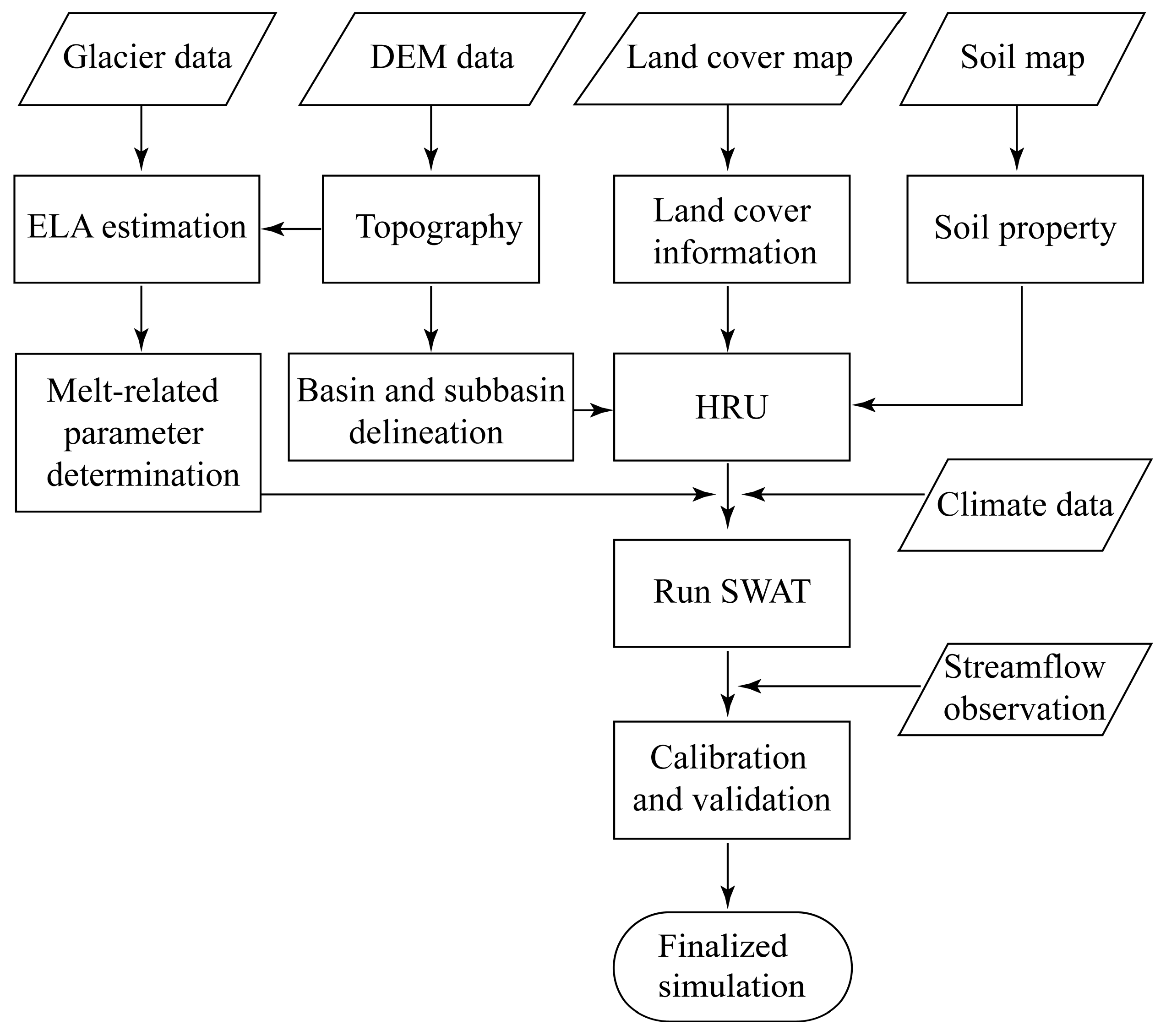
Figure 2.
Methodological flowchart for SWAT.
The main hydrological processes performed in SWAT can be divided into two major phases. The first of these is the land phase of the hydrological cycle, in which the amount of water flowing into the main channel is estimated for each subbasin. The runoff, evapotranspiration, melting processes, and soil–water processes are simulated in this phase. The second division is the channel phase of the hydrological cycle which can be defined as the movement of water through the channel network to the basin outlet [30]. Various methods are used to simulate these processes numerically and to estimate the key components of the catchment water balance. The soil conservation service curve number is an essential method, and is widely used for empirically estimating surface rainfall-runoff [40]. This estimation is primarily based on the land cover and soil type of the catchment. The SWAT model is capable of estimating the runoff from frozen soil if the temperature in the first soil layer is less than 0 °C [30]. The constant land cover and soil types were used in the present study due to their minimal variation over time (see Section 2.3 for more details). Meanwhile, the Penman–Monteith method [41,42] is satisfactory for estimating potential evapotranspiration by considering various climate parameters such as temperature, humidity, wind speed, and solar radiation. The kinematic storage method [43] is used to estimate lateral flow in soil layers, accounting for the variations in conductivity, slope, and soil water content of the catchment. Additionally, the variable storage routing method [44] is used to estimate the movement of water through the channel network by considering channel characteristics such as width, length, and slope within the catchment. Therefore, the selection of SWAT as the foundational model is underpinned by its notable attributes: its complicated preprocessing is made relatively accessible through ArcGIS 10.7.1 software add-ins and its computation is relatively efficient owing to the semi-distributed structure with fewer repetitive routines. Moreover, the existing literature has verified that SWAT performs well in reproducing the hydrological processes in mountainous and glacierized basins [39,45].
The snowfall and melting processes are important components of the hydrological cycle in the present study, since the Alaska catchment is partially covered by snow and ice. The SWAT model distinguishes between rainfall and snowfall based on a comparison of the near-surface air temperature and the threshold snowfall temperature (SFTMP). Snowfall occurs when the mean daily air temperature is lower than the SFTMP, and snow can accumulate until melting occurs. Melting begins when the air temperature is higher than the threshold snowmelt temperature (SMTMP). The SWAT model allows for spatial variations in precipitation and temperature by accounting for changes in elevation at the subbasin level. A maximum of ten elevation bands can be defined in SWAT. In each elevation band, the precipitation and temperature are modified based on two lapse rates, namely the temperature lapse (TLAPS) and precipitation lapse (PLAPS). Given that the elevation of glacierized areas in the Alaska catchment is mostly above 2000 m, ten elevation bands were established in the present study.
In the default setting of SWAT, melting calculations are based on a simplistic temperature-index method that does not account for ice melting. This is potentially problematic, given the considerable contribution of meltwater from glacierized areas. Therefore, the melting process in glacierized areas is additionally modified by separate calculations based on the equilibrium-line altitude (ELA). The ELA is a theoretical line where the annual mass balance is zero and represents the boundary between the accumulation and ablation zones of a glacier. In this study, the ELA was initially estimated by using the accumulation area ratio (AAR), which is the ratio between a glacier’s accumulation zone and its total area [46]. More specifically, based on the available AAR observational data [47] for glaciers in the Alaska catchment, the average AAR value was estimated to be 0.62. The glaciers in each basin were treated as a group, rather than as individual glaciers. Next, the elevation data for the glaciers were used, along with their outlines from the Randolph Glacier Inventory (RGI) 6.0 dataset [48], to conduct the ELA calculations of the glaciers within the five basins. As the glacial volume loss makes a relatively low contribution (6–10%) to the discharge [26,27,28], the glacierized areas are treated as constant during the estimation. The ELAs were therefore estimated as 1378, 1602, 1287, 1331, and 1542 m for glaciers in the Susitna, Copper, Alsek, Taku, and Stikine basins, respectively. The average ELA for the five basins was 1428 m, which is similar to the available observed mean ELA for Alaska glaciers (1363 ± 103 m) during 1982–2020 [49]. Finally, the estimated ELA in each basin was applied to divide the elevation bands into accumulation and ablation zones within the glacierized subbasins. The lowest elevation band of the ablation zone corresponds to the location where 90% of the glaciers’ coverage is reached.
Separate melt factors were established for the ablation and accumulation zones to determine the spatially distinct melting processes, based on the methods described by Omani et al. [45]. The parameters used to estimate the snowfall, snow accumulation, and melting processes at the subbasin level were given fixed values and were well constrained by previous research and physical interpretations [45,50,51]. Thus, for the non-glacier zone, the SFTMP and SMTMP were each set as 0 °C, the maximum snowmelt factor (SMFMX) on 21 June was set as 5 mm⋅H2O⋅°C−1⋅day−1, the minimum snowmelt factor (SMFMN) on December 21 was set as 3 mm⋅H2O⋅°C−1⋅day−1, and the snowpack temperature lag factor (TIMP) was set as 1. For the ablation zone, the SFTMP, SMTMP, SMFMX, SMFMN, and TIMP were 1 °C, 0.5 °C, 6 mm⋅H2O⋅°C−1⋅day−1, 3 mm⋅H2O⋅°C−1⋅day−1, and 0.05, respectively. For the accumulation zone, the corresponding values were 2 °C, 2 °C, 7 mm⋅H2O⋅°C−1⋅day−1, 4 mm⋅H2O⋅°C−1⋅day−1, and 0.01, respectively. Seasonal snow melt and summer ice melt mainly occur in the ablation zone, while permanent snow and ice undergo accumulation and melting in the accumulation zone. The initial glacier depth was set at 15,300 mm by averaging the thickness of the observed glaciers (RGI 6.0) within the Alaska catchment. Overall, while this approach does not fully capture the complexities of melting processes, such as the glacial dynamics and behavior of individual glaciers, it effectively accounts for the major accumulation and melting processes driven by temperature, considering spatial variability and using reasonable melting-related parameters based on the existing literature [39,45,50]. Despite its simplicity, the SWAT model in combination with the temperature-index approach is suitable for melting calculations.
2.3. Model Inputs
The model input data are listed in Table 1. The 30 m resolution DEM data, obtained from ASTER Global Digital Elevation Model version 3, were used in SWAT to delineate basins and subbasins, and to compute the flow directions of the river system. Land cover data with a resolution of 30 m were obtained from the North America Land Cover 2015. The Alaska catchment area was divided into 9 land cover types. The Food and Agriculture Organization (FAO) Digital Soil Map of the World [52], with a scale of 1:5,000,000, was used to classify the 18 soil types that could be directly used in the SWAT soil database.

Table 1.
The input data used in the SWAT model.
The land cover and soil inputs for SWAT were regarded as constant throughout the simulation, which could lead to uncertainties. However, no evidence that significantly contradicts the consideration of constant land cover and soil inputs was found in previous studies. More specifically, regarding the land cover distribution, most forested areas and other land cover types such as pasture, rangeland, built-up land, and cropland, did not undergo significant changes in northwestern North America, including in the Alaska catchment, during 1960–2020 [53,54,55]. Regarding the change in soil distribution, the process is more commonly long-term, while extreme and significant change can be brought about by short-term processes primarily associated with human activities. However, such short-term changes were found to be less evident in the Alaska catchment [56].
The meteorological data including daily precipitation (mm), maximum and minimum temperature (°C), solar radiation (MJ⋅m−2), relative humidity (%), and wind speed (m⋅s−1), were used to force the hydrological processes in the SWAT simulation. Notably, the meteorological data were obtained from two separate datasets, namely the climate forecast system reanalysis (CFSR, 1979–2013, [57]) and the climate forecast system version 2 operational data (CFSv2, 2011–2022, [58]). Nevertheless, the CFSv2 can be considered as an extension of the CFSR, which has been successfully applied to simulate the hydrological processes in North America [28,57,58]. Therefore, the dual datasets were used to force the discharge simulation in this study.
2.4. Model Calibration and Validation
In this study, the SWAT Calibration and Uncertainty Program (SWAT-CUP) was used to calibrate the model parameters [59]. SWAT-CUP is an interface that applies the Sequential Uncertainty Fitting (SUFI-2) algorithm to determine the parameter values and their uncertainties via sequential and fitting processes [59]. Although many parameters influence the discharge estimation in SWAT, the availability of adequate parameter values based on observation is limited. To avoid excessive tuning, fewer parameters should be considered, with more attention being paid to the features that they represent [60]. Therefore, the present study mainly focuses on the most influential parameters based on previous studies that used SWAT to estimate the discharge in snow and glacierized basins [39,45,61,62]. These parameters account for the primary hydrological processes within the study area, including the surface runoff, evapotranspiration, and groundwater flow processes, thereby ensuring the efficiency and accuracy of the model calibration. The calibrated parameters included the curve number (CN2), which is a key parameter for estimating surface runoff, as it directly influences the quantity of precipitation that becomes runoff. The available water capacity of the soil layer (SOL_AWC, mm⋅H2O⋅mm soil−1) and the soil evaporation compensation (ESCO) are crucial to soil moisture and evaporation processes. The minimum snow water content that corresponds to 100% snow cover (SNOCOVMX, mm⋅H2O) influences the areal depletion of snowpack coverage, which is essential for representing snowmelt timing and runoff volume. The threshold depth of water in the shallow aquifer required for return flow to occur (GWQMN, mm⋅H2O), the groundwater delay time (GW_DELAY, days), and the baseflow alpha factor (ALPHA_BF) play an important role in routing meltwater through the subsurface, affecting the hydrological response of the watershed. The TLAPS (°C⋅km−1,) and the PLAPS (mm⋅H2O⋅km−1) control the spatiotemporal distribution of precipitation, determining whether it falls as rain or snow. The model performance was evaluated by statistical metrics such as the Nash–Sutcliffe efficiency (NSE), the coefficient of determination (r2), and the percentage bias (PBIAS). The model result was considered acceptable when the critical threshold for each index was satisfied, i.e., NSE > 0.50, r2 > 0.70, and |PBIAS| < 25% [63]. Positive values of PBIAS indicate an underestimation bias in the model, while negative values indicate an overestimation bias. More detailed information on SWAT can be found in the official document [64].
In the present study, the model calibration and validation were performed using limited monthly observed streamflow data from the outlets of the five basins. The observed data were obtained from the Global Runoff Data Centre (https://portal.grdc.bafg.de/applications/public.html?publicuser=PublicUser#dataDownload/Home). The streamflow gauging positions are shown in Figure 1a, and the specific details are presented in Table S2. For the Susitna basin, the streamflow observations for 1982–1988 were used for calibration, and those for 1989–1992 were used for validation. For the Copper basin, the calibration period was 1982–1985 and the validation period was 1986–1990.9. For the Alsek basin, the calibration period was 1991.7–1997 and the validation period was 1998–2012.11. For the Taku basin, the calibration period was 1987.8–1997 and the validation period was 1998–2008. For the Stikine basin, the calibration period was 1982–1997 and the validation period was 1998–2005. The model configurations including the setup of elevation bands and the calibrated parameters in each of the five basins were subsequently projected to their adjacent ungauged basins for further discharge estimation, according to the principle of spatial proximity and hydrological similarity [65,66]. Specifically, the setup of the elevation bands and the calibrated parameters in the Susitna basin were projected to its neighboring basins, namely, ungauged basins No. 1, 2, and 3 (Figure 1a). Similarly, the setup from the Copper basin was applied to ungauged basin No. 4, those from the Alsek basin to ungauged basins No. 5 and 6, and those from the Stikine basin to ungauged basins No. 7 and 8.
The results of model calibration and validation are presented in Section 3.1. The estimated Alaska discharge is then discussed as a whole in Section 3.2, and for each of the five basins and the ungauged basins in Section 3.3. Here, the discharge characteristics for each of the five individual basins are discussed to provide a better understanding of the regional heterogeneity. Additionally, the integrated discharge from the ungauged basins is discussed and compared with that from the five basins.
2.5. Statistical Analysis
Herein, the trend in the Alaska discharge was assessed by using the non-parametric Mann–Kendall Test and Sen’s slope estimator. The Mann–Kendall Test is widely used to detect significant trends in time series datasets [67,68]. A trend exists when the statistical values satisfy p < 0.05 and |Zs| > 1.96. A positive Zs value indicates an increasing trend, while a negative Zs indicates a decreasing trend. The Sen’s slope estimator determines the slope of the trend, thereby indicating the rate of change [69]. Furthermore, the relationship between the long-term variations (5-year running means) in the Alaska discharge and the North Pacific Gyre Oscillation (NPGO) index [70] (i.e., the time series of the NPGO) is determined. The NPGO is suggested to be driven by sea surface wind variability associated with the NPO, which is an atmospheric variability characterized by a seesaw north–south dipole between the Aleutian Low and the North Pacific High. Therefore, the NPGO index is referred to as the oceanic expression of the NPO [70], and is used to reveal the connection between variations in the Alaska discharge and the NPO. Moreover, the annual Alaska discharge is compared with the sea surface salinity anomalies for 1984–2008 in the Alaskan Stream, as reported by Uehara et al. [12], to investigate the effects of the Alaska discharge on the oceanic characteristics in the North Pacific sector.
3. Results
3.1. Model Calibration and Validation
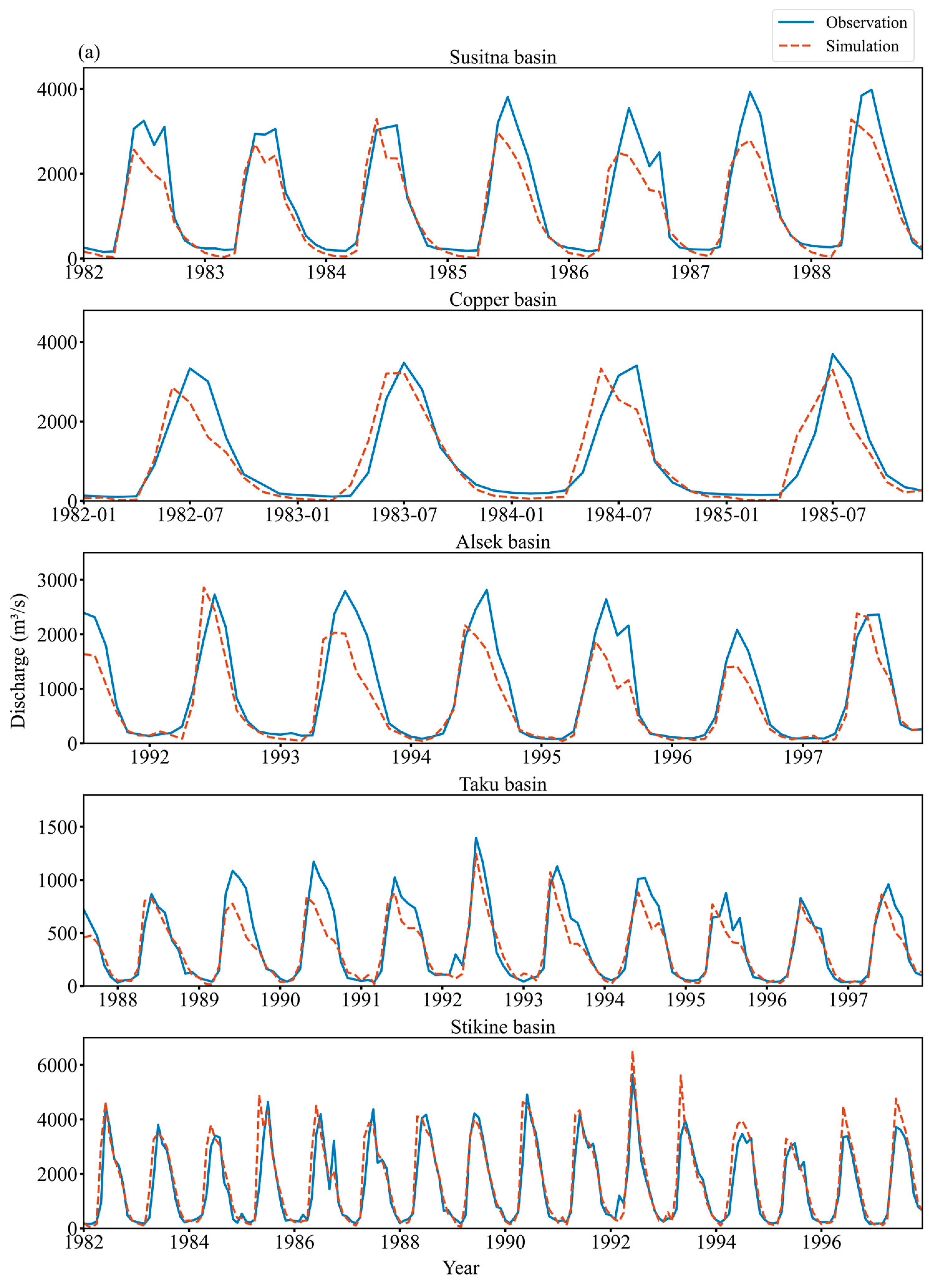
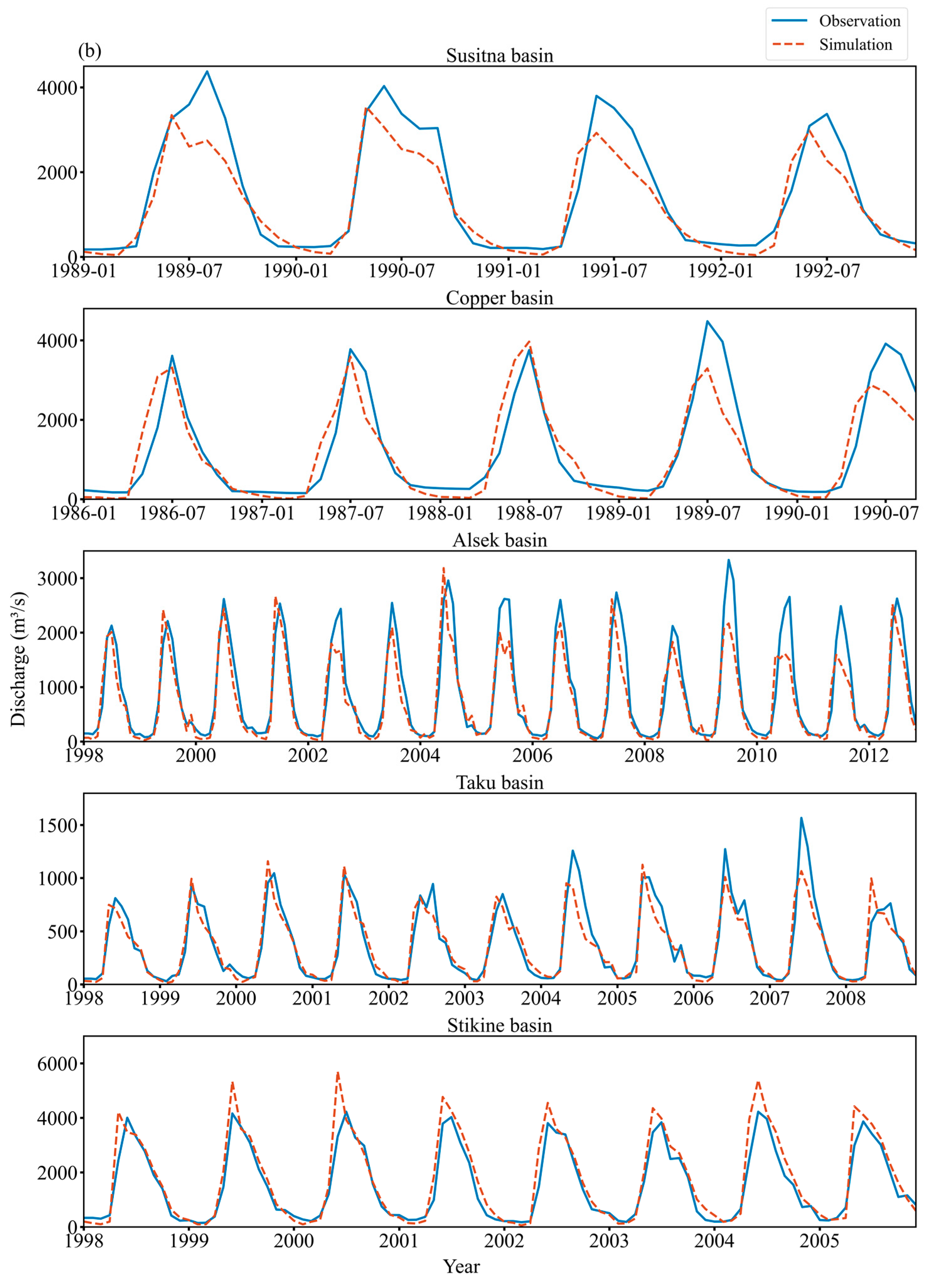
The default values for the selected parameters, the methods of adjustment used, and the final calibrated values over each basin are presented in Table 2. The parameters CN2 and SOL_AWC were adjusted by relative tests wherein the parameter value was multiplied by 1 + the given value in the Table, as indicated by r in the parameter designation. The other parameters were modified by replacement tests wherein the parameter value was replaced by the given value, as indicated by v in the parameter designation. The calibrated parameters are within reasonable ranges. Among the calibrated parameters, ALPHA_BF is the most sensitive across the five basins (Figure S2). The model’s performance varies significantly when ALPHA_BF, baseflow alpha factor, is adjusted within the range of −0.1–0.03, whereas the model tends to stabilize and deliver satisfactory performance when its value exceeds 0.03 (Figure S3). The calibration and validation performance indices for each basin are given in Table 3, which indicates that NSE values are greater than 0.5, r2 values are greater than 0.7, and PBIAS values are within ± 25%. These results statistically demonstrate an acceptable model performance. Indeed, the simulated discharge hydrograph in Figure 3a,b agrees well with observations during both the calibration and validation periods, especially in the Alsek, Taku, and Stikine basins, which have relatively longer observational datasets than the Susitna and Copper basins. However, the results indicate that the SWAT model underestimates the discharge from the Susitna, Copper, Alsek, and Taku basins, while it overestimates the Stikine basin, especially in summer (Figure 3 and Table 3). This can be primarily attributed to uncertainties in the meltwater estimation related to the catchment characteristics, particularly the topography. Compared to the other basins, the elevation bands of the Stikine basin are predominantly distributed at higher altitudes. Although the use of elevation bands in SWAT is acceptable for estimating snow-related processes and improving hydrological performance, it tends to slightly overestimate the snow accumulation and subsequent snowmelt in high-elevation regions and underestimate them in low-elevation regions, due to uncertainties arising from the linear variation in the temperature and precipitation lapse rates [39]. Moreover, the Susitna and Copper basins largely encompass areas with slopes of less than 15% (56% and 52% of the basin area, respectively). This relatively gentle slope may introduce uncertainties in the hydrological processes by reducing the surface runoff and increasing the soil water storage and evaporation during the simulated summer season. Despite several discrepancies in the hydrograph, the calibrated model is satisfactory for representing the discharge processes, and is therefore considered to be capable of estimating the discharge from the five basins.
Table 2.
The SWAT parameters and their values used for calibration.
Table 3.
The statistical results of the model performance.
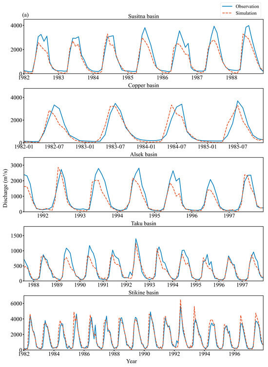
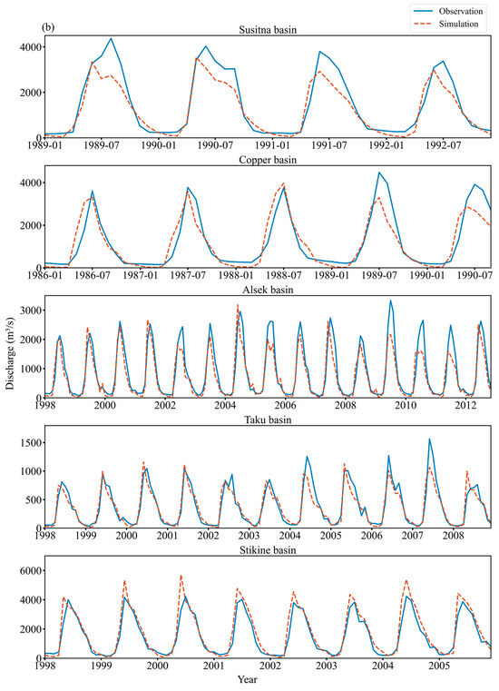
Figure 3.
Comparisons between simulated (red dashed lines) and observed (solid blue lines) monthly discharge values (m3⋅s−1) for the five basins: (a) calibration and (b) validation.
3.2. Alaska Discharge
The present subsection examines the combined Alaska discharge across the five basins plus the ungauged basins. The results in Figure 4 indicate that the annual Alaska discharge is approximately 14,396 ± 819 m3⋅s−1 during the period of 1982–2022, with a substantial contribution from meltwater (53%; Figure 5). In particular, the finding that melt runoff makes a significantly larger contribution to the total discharge than other contributors, such as direct rainfall, is consistent with the results of Neal et al. [26] and Beamer et al. [28]. However, the estimated annual discharge is slightly less than the 19,000–26,920 m3⋅s−1 reported in existing studies [15,26,27,28]. This is because the present study uses a smaller area to avoid uncertainties in the discharge estimation from flat areas near coastlines. SWAT is considered to be difficult to accurately delineate streams and catchments in such areas due to the presence of large but shallow depressions and subtle variations [71]. Additionally, the present study accounts for complicated hydrological processes in both the land phase and the channel phase, which may lead to a relatively high evapotranspiration and transmission loss.
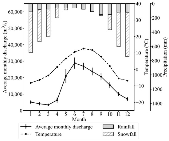
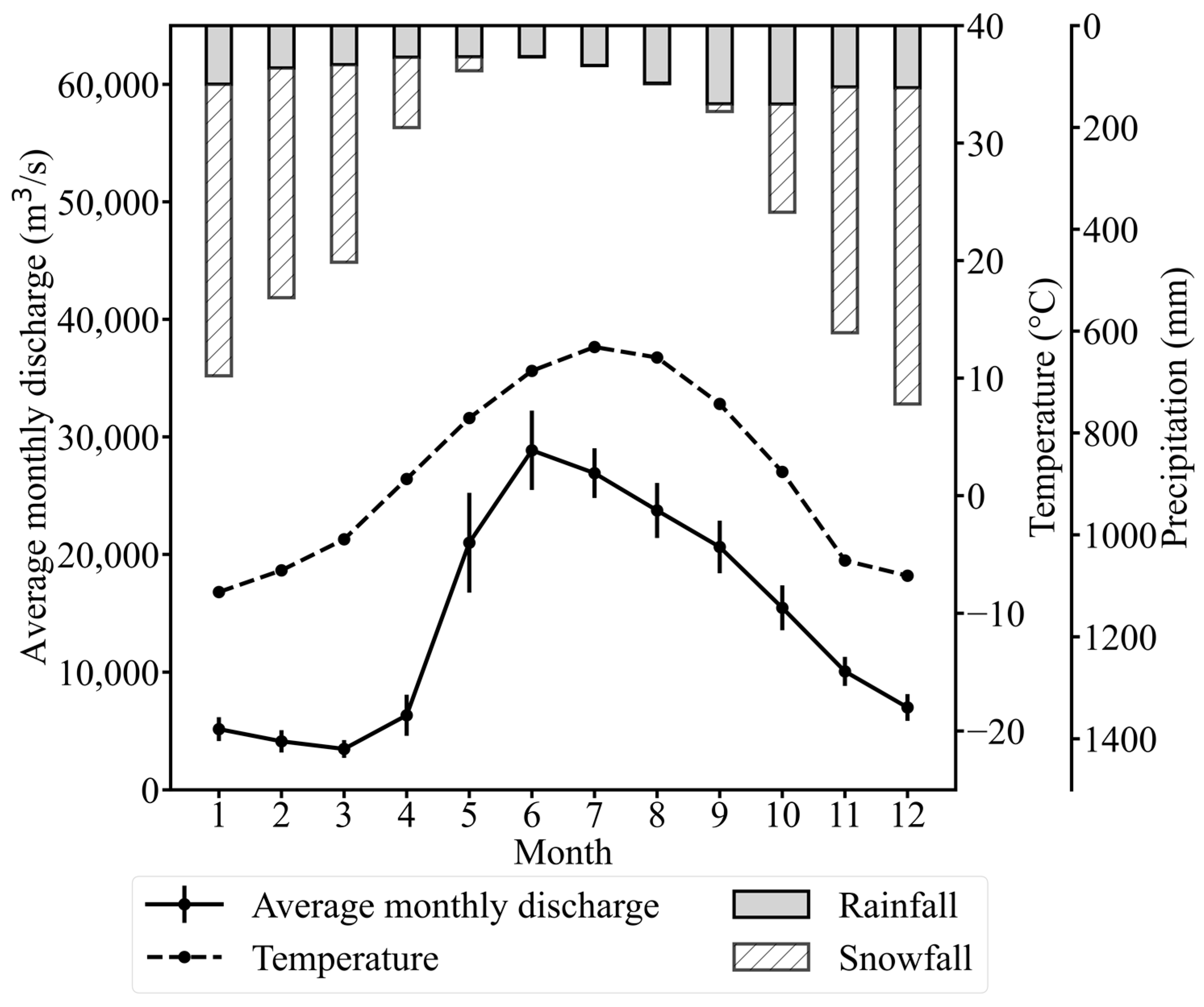
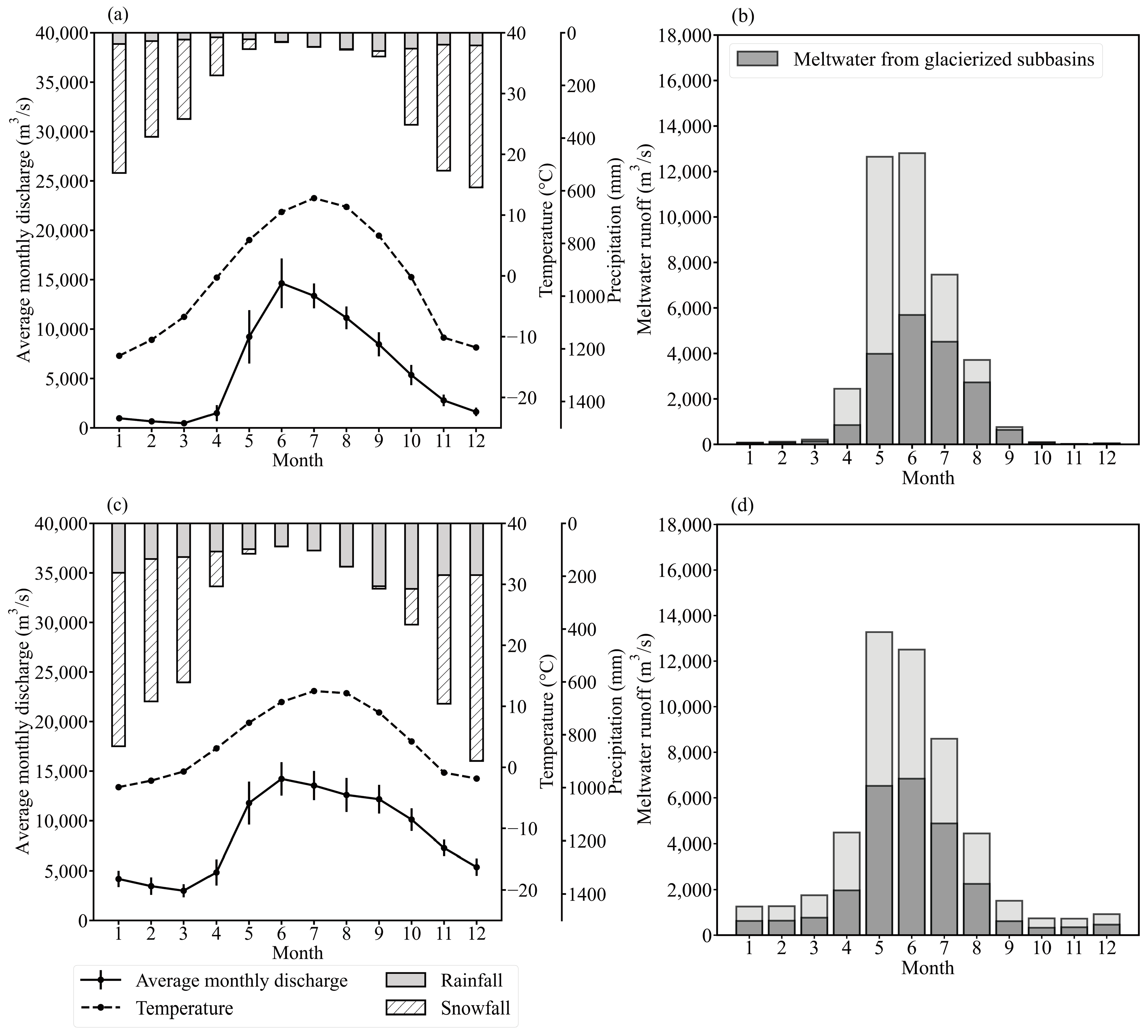
Figure 4.
The average monthly discharge (solid line), temperature (dashed line), rainfall (light gray bars), and snowfall (crosshatched bars) in the Alaska catchment.
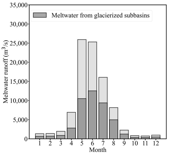
Figure 5.
Stacked plots of meltwater from the Alaska catchment (combined light and dark gray bars) and the meltwater from the glacierized areas (dark gray bars).
The monthly discharge exhibits a strong seasonal cycle in response to temperature variations (Figure 4). Specifically, the monthly discharge experiences a relatively constant average baseflow of 4252 ± 906 m3⋅s−1 from January to March compared to higher and more variable values in other seasons. This is primarily due to the low temperatures during January to March, which result in low meltwater (Figure 5). The Alaska discharge starts to increase rapidly in April as the temperature rises above 0 °C. This increase is closely related to the change in meltwater, which reaches its peak in May, thus leading to a peak discharge of approximately 30,000 m3⋅s−1 in June (Figure 4). Thereafter, the monthly discharge declines as the amount of meltwater decreases. This decline continues in the autumn, in contrast to the relatively high rainfall in late summer to early autumn, thereby indicating a less dominant impact of rainfall on the seasonal variability of discharge compared to the effect of temperature. During the melting season (i.e., from April to August), meltwater accounts for a significant proportion (77%) of the discharge (Figure 5). Additionally, during this period, the meltwater experiences an increasing contribution (from 40% in April to 60% in August) from glacierized areas. Notably, this growing contribution against the overall decrease in meltwater from June to August suggests a possible increase in the amount of ice melt in glacierized areas, in agreement with the results of Beamer et al. [28]. The decrease in discharge continues at a drastic rate (4135 m3⋅s−1⋅month−1) from September to November, with meltwater contributing only 5% to the discharge in November. Finally, the monthly discharge in December returns to its baseflow level as the temperature drops below 0 °C.
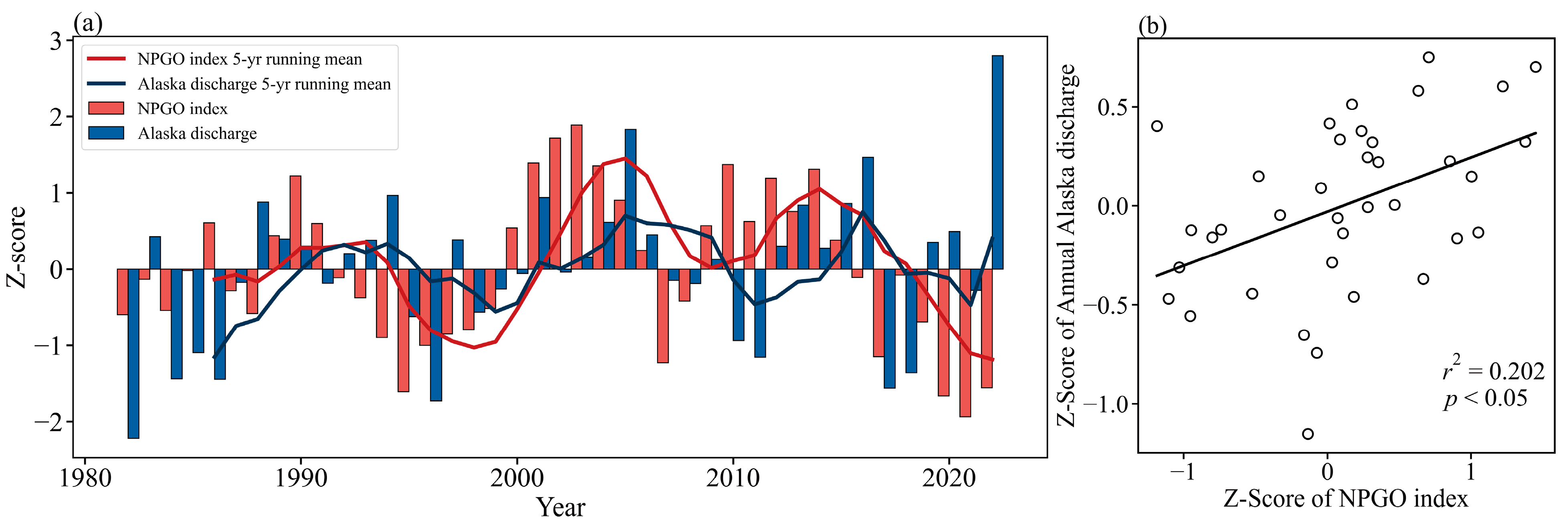
While no statistically significant trend is observed in the annual discharge during 1982–2022, the results in Figure 6a indicate a decadal pattern. Moreover, a statistically significant correlation is found between the five-year running mean of the NPGO index and the Alaska discharge when a two-year time lag between them is considered (p < 0.05, r2 = 0.202; Figure 6b). This implies that the decadal variation in the Alaska discharge is influenced by long-term variations in the NPO. As noted above, the surface wind variability associated with the NPO is a crucial driving force for the NPGO, thereby suggesting that the NPGO is regarded as the oceanic expression of the NPO [70]. The NPO consists of two typical phases, namely the Aleutian below phase and the Aleutian above phase [17,18], and can therefore be represented by the NPGO index. Specifically, positive phases of the NPGO index correspond to the Aleutian below phase of the NPO, and are characterized by an enhanced Aleutian low pressure over a relatively wide region, including coastal and interior North America, along with an enhanced North Pacific High across the subtropical North Pacific that develops and shifts poleward. This atmospheric variability leads to intensified westerlies that subsequently blow over the central Pacific, thereby resulting in increased storminess along with higher precipitation and milder winter temperatures along the west coast of North America [18,70]. Therefore, the hydrological processes may be subsequently influenced. Furthermore, the present study indicates that the NPO impacts the Alaska discharge with a lag of approximately two years. This time lag is deemed reasonable, as sea level pressure anomalies in the winter season primarily dominate precipitation in the form of snow, which may then influence melt runoff in the following seasons.
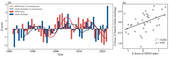
Figure 6.
The relationship between the interannual variation in the Alaska discharge from 1982 to 2022 and the NPGO index with a 2-year prior: (a) a bar chart showing the Z-scores of the annual Alaska discharge (blue) and the NPGO index (red), along with line profiles representing the 5-year running mean of the annual discharge (black), and the NPGO index (red); (b) a scatter plot of the Z-score of the 5-year running mean NPGO index versus the annual Alaska discharge.
In addition, the monthly Alaska discharge exhibits significant interannual variations and significant increases of 65.52 and 63.71 m3⋅s−1⋅yr−1 in summer (June–August) and autumn (September–November), respectively, during 1982–2022 (p < 0.05; Figure 7). These results can be attributed to the increases in winter snowfall and summer temperatures across the Alaska catchment. Specifically, it has been reported that the winter precipitation increased by roughly 4.9%⋅decade−1, and the summer temperature increased by around 0.42 °C⋅decade−1, during 1957–2021 [38].
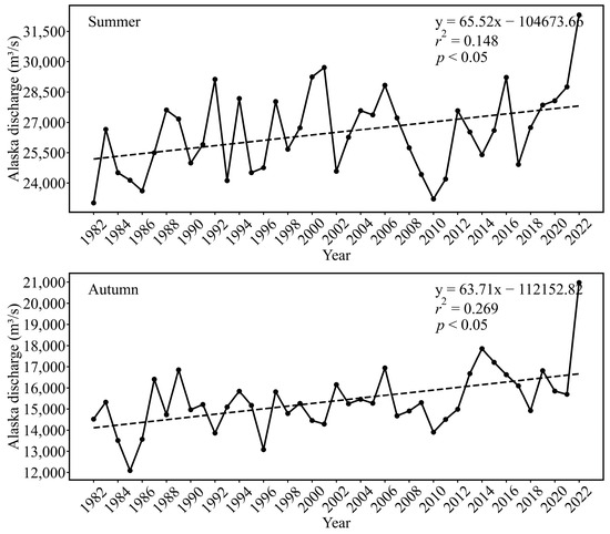
Figure 7.
The interannual variations (solid line) and trend (dashed line) of the Alaska discharge in summer and autumn during 1982–2022.
3.3. The Discharge of the Five Basins and the Ungauged Basins
Figure 8a,b show the total discharge from the five basins and the specific meltwater contribution, respectively, while the corresponding results for the ungauged basins are shown in Figure 8c,d. Thus, during 1982–2022, the total annual discharge from the five basins was approximately 5848 ± 533 m3⋅s−1 (0.03 m3⋅s−1⋅km−2), including a substantial contribution from meltwater (58%). Specifically, the freezing temperatures from January to March resulted in minimal meltwater (138 m3⋅s−1 on average) and low rainfall (34 mm on average), thus leading to an average baseflow of 701 m3⋅s−1. The discharge experienced a drastic increase from 1495 m3⋅s−1 in April to 9216 m3⋅s−1 in May, and reached a peak discharge of approximately 15,000 m3⋅s−1 in June. From June to August, although the rainfall increased, the discharge of the five basins declined by approximately 1749 m3⋅s−1⋅month−1 in response to a rapid decline in meltwater. During the melting season (from April to August), the monthly discharge was approximately 9970 m3⋅s−1, with a considerable contribution of approximately 78% from meltwater, 36% of which came from glacierized areas. From September to December, the discharge decreased to a baseflow level at a rate of 2309 m3⋅s−1⋅month−1 as the temperature declined to below 0 °C. While no statistically significant trend is detected in the total annual discharge from the five basins between 1982 and 2022, the total monthly discharge in January, August, September, and November experienced a significant increase (Table S3).
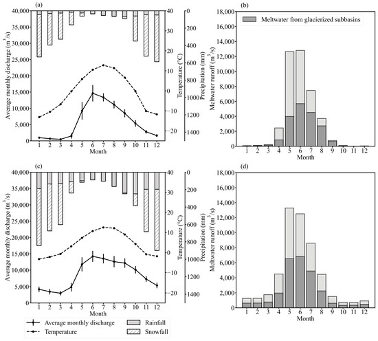
Figure 8.
(a) The total average monthly discharge from the five basins (solid line), along with the average monthly temperature (dashed line), rainfall (light gray bars), and snowfall (crosshatched bars). (b) Stacked plots of the total meltwater from the five basins (aggregate light and dark gray bars) and the meltwater from the glacierized areas (dark gray bars). (c,d) Same as (a,b) but for the ungauged basins.
Moreover, the ungauged basins (Figure 8c,d) deliver a larger contribution of 59% to the Alaska discharge, compared to 41% from the five basins (Figure 8a,b), despite having a smaller catchment area. This finding is in agreement with the results reported by Wang et al. [15]. The annual discharge of the ungauged basins is approximately 8548 ± 481 m3⋅s−1 (0.07 m3⋅s−1⋅km−2) during 1982–2022, with meltwater contributing approximately 50%. Specifically, the discharge in the ungauged basins from January to March is five times that of the five major basins. This is primarily because the temperature in the ungauged basins fluctuates more closely around 0 °C compared to that in the five basins, thereby resulting in more meltwater (1426 m3⋅s−1 on average) and rainfall (150 mm on average). Similarly to that from the five basins, the discharge from the ungauged basins begins to increase substantially in April as the temperature rises above 0 °C. However, the rate of increase from April to May is slower than that observed in the five basins, primarily due to the less drastic increase in temperature in the ungauged basins, which results in a smaller variation in meltwater. The discharge of the ungauged basins also reaches its peak in June, but at a lower rate than that in the five basins, due to a slight decrease in snowmelt during this period. From June to August, despite a slightly larger rainfall, the decrease in discharge continues at a rate of 810 m3⋅s−1⋅month−1. During the melting season (from April to August), the monthly discharge of the ungauged basins is approximately 11,396 m3⋅s−1, and again includes a larger contribution (76%) from meltwater than that received by the five basins. Of this contribution, 39% comes from glacierized areas. From August to October, the monthly discharge of the ungauged basins is approximately 11,627 m3⋅s−1, which is higher than that of the five basins due to the correspondingly higher rainfall and meltwater. The temperature drops below 0 °C from October to December, but remains higher than that in the five basins, thereby leading to relatively higher amounts of meltwater and, hence, higher baseflow. In addition, during this period, the higher rainfall contributes significantly to the higher baseflow in the ungauged basins relative to the five basins. While no statistically significant trend is detected in the annual discharge from 1982 to 2022, the monthly discharge from the ungauged basins exhibits a significant decreasing trend in May, and an increasing trend in August (Table S3).
Finally, the discharges from each of the five individual basins between 1982 and 2022 are shown in Figure 9, where differences in the quantity and variation are observed. The annual specific discharges from the Stikine, Taku, Susitna, Alsek, and Copper basins are 0.036, 0.031, 0.03, 0.029, and 0.027 m3⋅s−1⋅km−2, respectively. Thus, the specific discharge in the southern portion (Stikine and Taku basins) of the Alaska catchment is generally higher than that in the northern part (Susitna, Alsek, and Copper basins). This is predominantly due to a higher annual precipitation in the southern part. Additionally, the Stikine and Taku basins receive a higher contribution from groundwater (approximately 600 mm⋅yr−1) compared to the northern part. The lowest specific discharge is observed in the Copper basin, which may be due to the limited precipitation (approximately 1800 mm⋅yr−1) and low average temperature (below −2 °C).
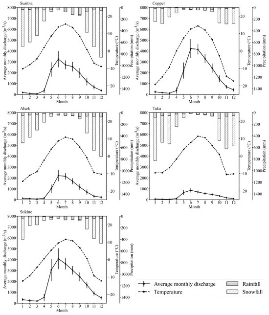
Figure 9.
The average monthly discharge (solid lines) and monthly temperature (dashed lines) for each of the five major basins, along with the rainfall (gray area) and snowfall (crosshatched area). The vertical error bars on the solid line indicate the range of one standard deviation.
In terms of the trends, only the Susitna basin exhibits an increase in the annual discharge during the period of 1982 to 2022. Further, the Copper, Alsek, and Taku basins each exhibit a decrease in the monthly discharge in April, while all basins except the Stikine basin exhibit an increasing trend during August (Table S4).
4. Discussion
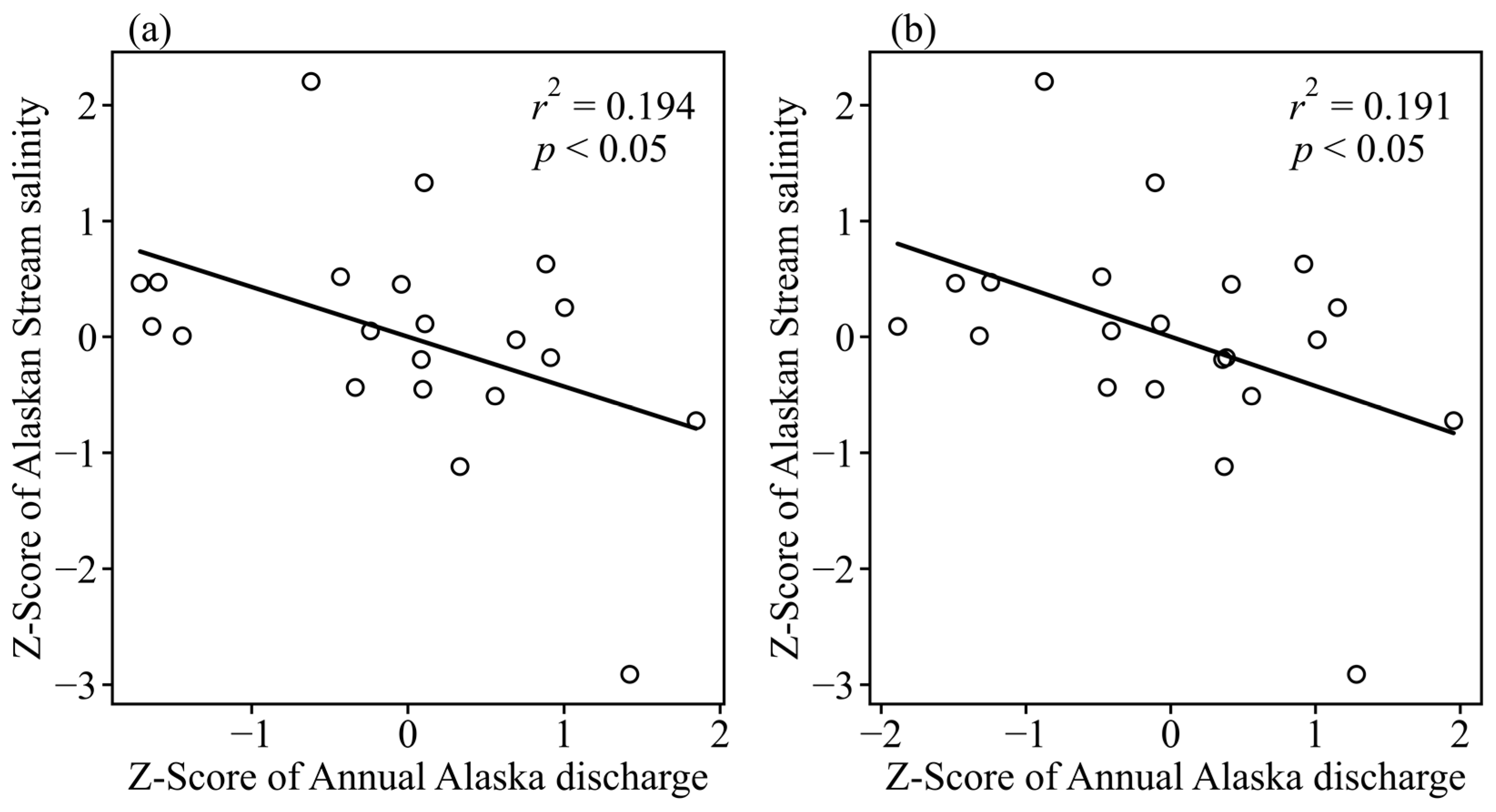
The freshwater discharge from the Alaska catchment may deliver cascading impacts on the neighboring ocean sector. After entering the GOA, the Alaska discharge primarily joins the Alaska Coastal Current (ACC). The ACC begins in the vicinity of the Washington–British Columbia border and travels at a speed of about 0.1 m⋅s−1 along the coast, carrying precipitation over the ocean and continental discharge into the Bering Sea [72,73]. The ACC flows westward and southward along the Alaska coast and partially enters the Alaskan Stream before entering the Bering Sea through Unimak Pass [74,75]. As shown in Figure 10, the interannual variation of sea surface salinity in the Alaskan Stream during the period of 1984–2008 exhibits a statistical correlation with the variation in the annual Alaska discharge when considering a time lag, thereby suggesting that the Alaska discharge may impact the Alaskan Stream with a delay of two or three months (p < 0.05, r2 = 0.2). Although these time lags are derived from statistical results, they are reasonable considering that the average distance covered by the ACC in going from the coastal regions of the GOA to the location of the Alaskan Stream is more than 500 km. In addition to the freshening effect of the continental discharge, other factors such as upwelling and current advection may also affect the seawater salinity of the Alaskan Stream [76], thereby rendering the correlation less prominent. This significant correlation indicates that the Alaska discharge may influence the current circulation of the North Pacific Ocean through its impacts on the characteristics of the surrounding ocean.
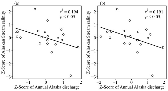
Figure 10.
Scatter charts showing the correlation between the annual Alaska discharge and sea surface salinity anomalies in the Alaskan Stream with time lags of (a) two months and (b) three months.
5. Conclusions
The Alaska discharge is characterized by large quantity and considerable variability, due to the complex interplay between climatic variations and mountainous topography, delivering cascading impacts on the coastal circulation beyond the regional scale. The present study estimated the quantity and variability of the continental discharge from the Alaska catchments under the continual fluctuations in temperature and precipitation in recent decades. The Alaska discharge was effectively estimated by using a process-based hydrological model known as the Soil and Water Assessment Tool (SWAT) with modified melting processes. During the estimation, SWAT was able to account for the complex spatial variability of land cover and soil features at the basin scale. The primary advances of this study are as follows: (i) an update on the estimated discharge during recent years, (ii) an analysis of the temporospatial variabilities in discharge, and (iii) a first discussion on the relationship between continental discharge and large-scale oceanic circulation in this region.
The results indicate an annual Alaska discharge of 14,396 ± 819 m3⋅s−1, with a strong seasonal variability. In detail, the discharge maintains a baseflow level from January to March, when the temperature is well below freezing, and begins to increase drastically in April in response to rising temperatures. A peak flow of approximately 30,000 m3⋅s−1 occurs in June, after which the discharge decreases swiftly despite the relatively high rainfall during late summer to early autumn, and resumes its baseflow level in December. Meltwater plays an important role in the discharge accumulation process, contributing approximately 53% to the annual discharge and exerting a more dominant control than rainfall on the seasonal discharge variation. Notably, the ungauged basins provide a larger contribution of roughly 59% to the Alaska discharge, despite having a smaller catchment area, whereas the five basins provide the remaining 41%. The interannual variation in the Alaska discharge experiences an increasing trend for the summer and autumn, while the annual discharge exhibits no significant trend. The interannual variation in the Alaska discharge from 1982 to 2022 exhibits a decadal trend. Additionally, a significant correlation is found between the 5-year running mean of the Alaska discharge and the NPGO index, thereby suggesting that the NPO, a large-scale sea level pressure anomaly variation over the North Pacific, may affect the decadal variations in the Alaska discharge.
This study revealed an unprecedented significant correlation between the interannual variation in the Alaska discharge and sea surface salinity in the Alaskan Stream. The salinity anomalies potentially impact the overturning circulation through the current pathway, since it is situated in the upper branch of the pathway. The correlation becomes significant when a time lag of two or three months is assumed, which is reasonable considering the distance between the Alaska coastal outlets and the Alaskan Stream, along with the traveling speed of sea currents. Therefore, it is concluded that the regional discharge from the Alaska catchment could impact the variations in seawater anomalies in the North Pacific sector. Overall, the present study investigated the connection between large-scale climatic variations, Alaska discharge variations, and oceanic processes, which is expected to provide a broader understanding of the atmosphere–land–ocean relationship, especially in recent years.
Nevertheless, the present study has two major limitations. Firstly, while the temperature-index approach used to calculate meltwater is efficient, it is fairly simple. This method can be regarded as adequate for the monthly simulation presented herein, but a more complex method with high spatial resolution should be applied for the glacierized area. Secondly, parameterization might be improved based on more observation records in the calibration process for further improvement.
Supplementary Materials
The following supporting information can be downloaded at: https://www.mdpi.com/article/10.3390/w16182690/s1, Figure S1: A schematic diagram of a hypothesized salt pathway in association with an overturning from the surface flow in the subarctic gyre (orange arrows) to the intermediate layer (blue arrow) in the North Pacific Ocean; Figure S2: Results of sensitivity analysis by SWAT-CUP in the Alsek basin; Figure S3: Dotty plot of the parameter ALPHA_BF in the Alsek basin; Table S1: Details of land cover classifications; Table S2: The observational streamflow data used for model calibration and validation; Table S3: A summary of the Mann–Kendall test (MK Zs) and the Sen’s slope (SS) estimator results for the monthly discharge in the five basins and the ungauged basins; Table S4: A summary of the Mann–Kendall test (MK Zs) and the Sen’s slope (SS) estimator results for the average monthly discharge in the five individual basins.
Author Contributions
Conceptualization, P.X., M.S. and H.M.; data curation, P.X.; formal analysis, P.X.; funding acquisition, P.X. and H.M.; investigation, P.X. and M.S.; methodology, P.X., M.S., H.M. and T.S.; project administration, H.M.; resources, P.X. and H.M.; software, P.X. and M.S.; supervision, H.M. and T.S.; validation, P.X. and M.S.; visualization, P.X. and M.S.; writing—original draft, P.X. and M.S.; writing–review and editing, P.X., M.S., H.M. and T.S. All authors have read and agreed to the published version of the manuscript.
Funding
This work was supported by Grants-in-Aid for Scientific Research, the Japan Society for the Promotion of Science (JSPS KAKENHI), No.21H01154 and 21H05056, and the Japan Science and Technology Agency Support for Pioneering Research Initiated by the Next Generation (JST SPRING), Grant Number JPMJSP 2119.
Data Availability Statement
Data available on request due to privacy.
Conflicts of Interest
The authors declare no conflicts of interest.
References
- Syed, T.H.; Famiglietti, J.S.; Chambers, D.P.; Willis, J.K.; Hilburn, K. Satellite-Based Global-Ocean Mass Balance Estimates of Interannual Variability and Emerging Trends in Continental Freshwater Discharge. Proc. Natl. Acad. Sci. USA 2010, 107, 17916–17921. [Google Scholar] [CrossRef]
- Cloern, J.E.; Alpine, A.E.; Cole, B.E.; Wong, R.L.J.; Arthur, J.F.; Ball, M.D. River Discharge Controls Phytoplankton Dynamics in the Northern San Francisco Bay Estuary. Estuar. Coast. Shelf Sci. 1983, 16, 415–429. [Google Scholar] [CrossRef]
- Masotti, I.; Aparicio-Rizzo, P.; Yevenes, M.A.; Garreaud, R.; Belmar, L.; Farías, L. The Influence of River Discharge on Nutrient Export and Phytoplankton Biomass off the Central Chile Coast (33°–37°S): Seasonal Cycle and Interannual Variability. Front. Mar. Sci. 2018, 5, 423. [Google Scholar] [CrossRef]
- Wetz, M.S.; Hutchinson, E.A.; Lunetta, R.S.; Paerl, H.W.; Christopher Taylor, J. Severe Droughts Reduce Estuarine Primary Productivity with Cascading Effects on Higher Trophic Levels. Limnol. Oceanogr. 2011, 56, 627–638. [Google Scholar] [CrossRef]
- Dai, A.; Trenberth, K.E. Estimates of Freshwater Discharge from Continents: Latitudinal and Seasonal Variations. J. Hydrometeorol. 2002, 3, 660–687. [Google Scholar] [CrossRef]
- Trenberth, K.E.; Smith, L.; Qian, T.; Dai, A.; Fasullo, J. Estimates of the Global Water Budget and Its Annual Cycle Using Observational and Model Data. J. Hydrometeorol. 2007, 8, 758–769. [Google Scholar] [CrossRef]
- Rahmstorf, S. Thermohaline Circulation: The Current Climate. Nature 2003, 421, 699. [Google Scholar] [CrossRef]
- Itoh, M.; Ohshima, K.I.; Wakatsuchi, M. Distribution and Formation of Okhotsk Sea Intermediate Water: An Analysis of Isopycnal Climatological Data. J. Geophys. Res. Ocean. 2003, 108, 3258. [Google Scholar] [CrossRef]
- Nakatsuka, T.; Toda, M.; Kawamura, K.; Wakatsuchi, M. Dissolved and Particulate Organic Carbon in the Sea of Okhotsk: Transport from Continental Shelf to Ocean Interior. J. Geophys. Res. Ocean. 2004, 109, C09S14. [Google Scholar] [CrossRef]
- Nishioka, J.; Nakatsuka, T.; Watanabe, Y.W.; Yasuda, I.; Kuma, K.; Ogawa, H.; Ebuchi, N.; Scherbinin, A.; Volkov, Y.N.; Shiraiwa, T.; et al. Intensive Mixing along an Island Chain Controls Oceanic Biogeochemical Cycles. Glob. Biogeochem. Cycles 2013, 27, 920–929. [Google Scholar] [CrossRef]
- Whitney, F.A.; Bograd, S.J.; Ono, T. Nutrient Enrichment of the Subarctic Pacific Ocean Pycnocline. Geophys. Res. Lett. 2013, 40, 2200–2205. [Google Scholar] [CrossRef]
- Uehara, H.; Kruts, A.A.; Mitsudera, H.; Nakamura, T.; Volkov, Y.N.; Wakatsuchi, M. Remotely Propagating Salinity Anomaly Varies the Source of North Pacific Ventilation. Prog. Oceanogr. 2014, 126, 80–97. [Google Scholar] [CrossRef]
- Shi, M.; Shiraiwa, T.; Mitsudera, H.; Muravyev, Y. Estimation of Freshwater Discharge from the Kamchatka Peninsula to Its Surrounding Oceans. J. Hydrol. Reg. Stud. 2021, 36, 100836. [Google Scholar] [CrossRef]
- Royer, T.C.; Grosch, C.E.; Mysak, L.A. Interdecadal Variability of Northeast Pacific Coastal Freshwater and Its Implications on Biological Productivity. Prog. Oceanogr. 2001, 49, 95–111. [Google Scholar] [CrossRef]
- Wang, J.; Jin, M.; Musgrave, D.L.; Ikeda, M. A Hydrological Digital Elevation Model for Freshwater Discharge into the Gulf of Alaska. J. Geophys. Res. Ocean. 2004, 109, C07009. [Google Scholar] [CrossRef]
- Kunkel, K.E.; Stevens, L.E.; Stevens, S.E.; Sun, L.; Janssen, E.; Wuebbles, D.; Hilberg, S.D.; Timlin, M.S.; Stoecker, L.; Westcott, N.; et al. Regional Climate Trends and Scenarios for the U.S. National Climate Assessment Part 3. Climate of the Midwest U.S.; NOAA Technical Report NESDIS 142-3; U.S. Department of Commerce, National Oceanic and Atmospheric Administration (NOAA), National Environmental, Satellite, Data, and Information Service: Silver Spring, MD, USA, 2013.
- Rogers, J.C. The North Pacific Oscillation. J. Climatol. 1981, 1, 39–57. [Google Scholar] [CrossRef]
- Linkin, M.E.; Nigam, S. The North Pacific Oscillation–West Pacific Teleconnection Pattern: Mature-Phase Structure and Winter Impacts. J. Clim. 2008, 21, 1979–1997. [Google Scholar] [CrossRef]
- D’Agnese, F.; Faunt, C.; Turner, A. Using Remote Sensing and GIS Techniques to Estimate Discharge and Recharge Fluxes for the Death Valley Regional Groundwater Flow System, USA. In Proceedings of the HydroGIS’96 Conference, Vienna, Austria, 16–19 April 1996. [Google Scholar]
- Dobriyal, P.; Badola, R.; Tuboi, C.; Hussain, S.A. A Review of Methods for Monitoring Streamflow for Sustainable Water Resource Management. Appl. Water Sci. 2017, 7, 2617–2628. [Google Scholar] [CrossRef]
- Gleason, C.J.; Durand, M.T. Remote Sensing of River Discharge: A Review and a Framing for the Discipline. Remote Sens. 2020, 12, 1107. [Google Scholar] [CrossRef]
- Todini, E. Hydrological Catchment Modelling: Past, Present and Future. Hydrol. Earth Syst. Sci. 2007, 11, 468–482. [Google Scholar] [CrossRef]
- Ahmed, M.I.; Stadnyk, T.; Pietroniro, A.; Awoye, H.; Bajracharya, A.; Mai, J.; Tolson, B.A.; Shen, H.; Craig, J.R.; Gervais, M.; et al. Learning from Hydrological Models’ Challenges: A Case Study from the Nelson Basin Model Intercomparison Project. J. Hydrol. 2023, 623, 129820. [Google Scholar] [CrossRef]
- Anees, M.T.; Abdullah, K.; Nawawi, M.N.M.; Ab Rahman, N.N.N.; Piah, A.R.M.; Zakaria, N.A.; Syakir, M.I.; Mohd Omar, A.K. Numerical Modeling Techniques for Flood Analysis. J. Afr. Earth Sci. 2016, 124, 478–486. [Google Scholar] [CrossRef]
- Maxwell, R.M.; Putti, M.; Meyerhoff, S.; Delfs, J.-O.; Ferguson, I.M.; Ivanov, V.; Kim, J.; Kolditz, O.; Kollet, S.J.; Kumar, M.; et al. Surface-Subsurface Model Intercomparison: A First Set of Benchmark Results to Diagnose Integrated Hydrology and Feedbacks. Water Resour. Res. 2014, 50, 1531–1549. [Google Scholar] [CrossRef]
- Neal, E.G.; Hood, E.; Smikrud, K. Contribution of Glacier Runoff to Freshwater Discharge into the Gulf of Alaska. Geophys. Res. Lett. 2010, 37, L06404. [Google Scholar] [CrossRef]
- Hill, D.F.; Bruhis, N.; Calos, S.E.; Arendt, A.; Beamer, J. Spatial and Temporal Variability of Freshwater Discharge into the Gulf of Alaska. J. Geophys. Res. Ocean. 2015, 120, 634–646. [Google Scholar] [CrossRef]
- Beamer, J.P.; Hill, D.F.; Arendt, A.; Liston, G.E. High-Resolution Modeling of Coastal Freshwater Discharge and Glacier Mass Balance in the Gulf of Alaska Watershed. Water Resour. Res. 2016, 52, 3888–3909. [Google Scholar] [CrossRef]
- Arnold, J.G.; Srinivasan, R.; Muttiah, R.S.; Williams, J.R. Large Area Hydrologic Modeling and Assessment Part I: Model Development1. JAWRA J. Am. Water Resour. Assoc. 1998, 34, 73–89. [Google Scholar] [CrossRef]
- Neitsch, S.; Arnold, J.; Kinry, J.R.; Williams, J.R. Soil and Water Assessment Tool Theoretical Documentation Version 2009; Texas Water Resources Institute: College Station, TX, USA, 2011. [Google Scholar]
- LP DAAC. NASA/METI/AIST/Japan Spacesystems and U.S./Japan ASTER Science Team ASTER Global Digital Elevation Model V003; LP DAAC: Sioux Falls, SD, USA, 2019. [Google Scholar] [CrossRef]
- Commission for Environmental Cooperation (CEC). “2015 Land Cover of North America at 30 Meters”. Canada Centre for Remote Sensing (CCRS)/Canada Centre for Mapping and Earth Observation (CCMEO), Natural Resources Canada (NRCan), U.S. Geological Survey (USGS), Comisión Nacional Para el Conocimiento y Uso de la Biodiversidad (CONABIO), Comisión Nacional Forestal (CONAFOR), Instituto Nacional de Estadística y Geografía (INEGI). Ed. 2.0, Raster Digital Data [30-m]. 2020. Available online: http://www.cec.org/nalcms (accessed on 17 July 2024).
- Bieniek, P.A.; Bhatt, U.S.; Thoman, R.L.; Angeloff, H.; Partain, J.; Papineau, J.; Fritsch, F.; Holloway, E.; Walsh, J.E.; Daly, C.; et al. Climate Divisions for Alaska Based on Objective Methods. J. Appl. Meteorol. Climatol. 2012, 51, 1276–1289. [Google Scholar] [CrossRef]
- Kottek, M.; Grieser, J.; Beck, C.; Rudolf, B.; Rubel, F. World Map of the Köppen-Geiger Climate Classification Updated. Meteorol. Z. 2006, 15, 259–263. [Google Scholar] [CrossRef]
- Beck, H.E.; Zimmermann, N.E.; McVicar, T.R.; Vergopolan, N.; Berg, A.; Wood, E.F. Present and Future Köppen-Geiger Climate Classification Maps at 1-Km Resolution. Sci. Data 2018, 5, 180214. [Google Scholar] [CrossRef]
- Wendler, G.; Galloway, K.; Stuefer, M. On the Climate and Climate Change of Sitka, Southeast Alaska. Theor. Appl. Clim. 2016, 126, 27–34. [Google Scholar] [CrossRef]
- Lader, R.; Bhatt, U.S.; Walsh, J.E.; Rupp, T.S.; Bieniek, P.A. Two-Meter Temperature and Precipitation from Atmospheric Reanalysis Evaluated for Alaska. J. Appl. Meteorol. Climatol. 2016, 55, 901–922. [Google Scholar] [CrossRef]
- Ballinger, T.J.; Bhatt, U.S.; Bieniek, P.A.; Brettschneider, B.; Lader, R.T.; Littell, J.S.; Thoman, R.L.; Waigl, C.F.; Walsh, J.E.; Webster, M.A. Alaska Terrestrial and Marine Climate Trends, 1957–2021. J. Clim. 2023, 36, 4375–4391. [Google Scholar] [CrossRef]
- Grusson, Y.; Sun, X.; Gascoin, S.; Sauvage, S.; Raghavan, S.; Anctil, F.; Sáchez-Pérez, J.-M. Assessing the Capability of the SWAT Model to Simulate Snow, Snow Melt and Streamflow Dynamics over an Alpine Watershed. J. Hydrol. 2015, 531, 574–588. [Google Scholar] [CrossRef]
- SCS (Soil Conservation Service) National Engineering Handbook, Section 4: Hydrology; Soil Conservation Service, US Department of Agriculture, The Service: Washington, DC, USA, 1972.
- Monteith, J.L. Evaporation and Environment. Symp. Soc. Exp. Biol. 1965, 19, 205–234. [Google Scholar]
- Allen, R.G.; Jensen, M.E.; Wright, J.L.; Burman, R.D. Operational Estimates of Reference Evapotranspiration. Agron. J. 1989, 81, 650–662. [Google Scholar] [CrossRef]
- Sloan, P.; Moore, I.; Coltharp, G.; Eigel, J. Modeling Surface and Subsurface Stormflow on Steeply-Sloping Forested Watersheds. KWRRI Res. Rep. 1983. [Google Scholar] [CrossRef]
- Jimmy, R. Williams Flood Routing with Variable Travel Time or Variable Storage Coefficients. Trans. ASAE 1969, 12, 100–103. [Google Scholar] [CrossRef]
- Omani, N.; Srinivasan, R.; Karthikeyan, R.; Smith, P.K. Hydrological Modeling of Highly Glacierized Basins (Andes, Alps, and Central Asia). Water 2017, 9, 111. [Google Scholar] [CrossRef]
- Cogley, J.G.; Hock, R.; Rasmussen, L.A.; Arendt, A.A.; Bauder, A.; Braithwaite, R.J.; Jansson, P.; Kaser, G.; Möller, M.; Nicholson, L.; et al. Glossary of Glacier Mass Balance and Related Terms; IHP-VII Technical Documents in Hydrology No. 86; UNESCO-IHP: Paris, France, 2011. [Google Scholar] [CrossRef]
- Mernild, S.H.; Lipscomb, W.H.; Bahr, D.B.; Radić, V.; Zemp, M. Global Glacier Changes: A Revised Assessment of Committed Mass Losses and Sampling Uncertainties. Cryosphere 2013, 7, 1565–1577. [Google Scholar] [CrossRef]
- RGI Consortium. Randolph Glacier Inventory—A Dataset of Global Glacier Outlines, Version 6; [Indicate subset used]; NSIDC National Snow and Ice Data Center: Boulder, CO, USA, 2017. [Google Scholar] [CrossRef]
- Ohmura, A.; Boettcher, M. On the Shift of Glacier Equilibrium Line Altitude (ELA) under the Changing Climate. Water 2022, 14, 2821. [Google Scholar] [CrossRef]
- Omani, N.; Srinivasan, R.; Smith, P.K.; Karthikeyan, R. Glacier Mass Balance Simulation Using SWAT Distributed Snow Algorithm. Hydrol. Sci. J. 2017, 62, 546–560. [Google Scholar] [CrossRef]
- Andrianaki, M.; Shrestha, J.; Kobierska, F.; Nikolaidis, N.P.; Bernasconi, S.M. Assessment of SWAT Spatial and Temporal Transferability for a High-Altitude Glacierized Catchment. Hydrol. Earth Syst. Sci. 2019, 23, 3219–3232. [Google Scholar] [CrossRef]
- Food and Agriculture Organization of the United Nations. FAO-UNESCO Soil Map of the World 1:5,000,000; UNESCO: Paris, France, 1974; ISBN 978-92-3-101125-2. [Google Scholar]
- Biswas, T.; Walterman, M.; Maus, P.; Megown, K.A.; Healey, S.P.; Brewer, K. Assessment of Land Use Change in the Coterminous United States and Alaska for Global Assessment of Forest Loss Conducted by the Food and Agricultural Organization of the United Nations. In Moving from Status to Trends: Forest Inventory and Analysis (FIA) Symposium 2012; 2012 December 4–6; Baltimore, MD. Gen. Tech. Rep. NRS-P-105; Morin, R.S., Liknes, G.C., Eds.; U.S. Department of Agriculture, Forest Service, Northern Research Station: Newtown Square, PA, USA, 2012; pp. 37–45. [Google Scholar]
- Winkler, K.; Fuchs, R.; Rounsevell, M.; Herold, M. Global Land Use Changes Are Four Times Greater than Previously Estimated. Nat. Commun. 2021, 12, 2501. [Google Scholar] [CrossRef] [PubMed]
- Potapov, P.; Turubanova, S.; Hansen, M.C.; Tyukavina, A.; Zalles, V.; Khan, A.; Song, X.-P.; Pickens, A.; Shen, Q.; Cortez, J. Global Maps of Cropland Extent and Change Show Accelerated Cropland Expansion in the Twenty-First Century. Nat. Food 2022, 3, 19–28. [Google Scholar] [CrossRef]
- Montanarella, L.; Pennock, D.; McKenzie, N.; Alavipanah, S.K.; Alegre, J.; Alshankiti, A.; Arrouays, D.; Aulakh, M.; Badraoui, M.; Baptista, I.; et al. The Status of the World’s Soil Resources (Technical Summary); FAO: Rome, Italy, 2015. [Google Scholar]
- Saha, S.; Moorthi, S.; Pan, H.-L.; Wu, X.; Wang, J.; Nadiga, S.; Tripp, P.; Kistler, R.; Woollen, J.; Behringer, D.; et al. The NCEP Climate Forecast System Reanalysis. Bull. Am. Meteorol. Soc. 2010, 91, 1015–1058. [Google Scholar] [CrossRef]
- Saha, S.; Moorthi, S.; Wu, X.; Wang, J.; Nadiga, S.; Tripp, P.; Behringer, D.; Hou, Y.-T.; Chuang, H.; Iredell, M.; et al. The NCEP Climate Forecast System Version 2. J. Clim. 2014, 27, 2185–2208. [Google Scholar] [CrossRef]
- Abbaspour, K.C.; Yang, J.; Maximov, I.; Siber, R.; Bogner, K.; Mieleitner, J.; Zobrist, J.; Srinivasan, R. Modelling Hydrology and Water Quality in the Pre-Alpine/Alpine Thur Watershed Using SWAT. J. Hydrol. 2007, 333, 413–430. [Google Scholar] [CrossRef]
- Shi, M.; Shiraiwa, T. Estimating Future Streamflow under Climate and Land Use Change Conditions in Northeastern Hokkaido, Japan. J. Hydrol. Reg. Stud. 2023, 50, 101555. [Google Scholar] [CrossRef]
- Fontaine, T.; Cruickshank, T.; Arnold, J.; Hotchkiss, R. Development of a Snowfall-Snowmelt Routine for Mountainous Terrain for the Soil Water Assessment Tool (SWAT). J. Hydrol. 2002, 262, 209–223. [Google Scholar] [CrossRef]
- Neupane, R.P.; Adamowski, J.F.; White, J.D.; Kumar, S. Future Streamflow Simulation in a Snow-Dominated Rocky Mountain Headwater Catchment. Hydrol. Res. 2017, 49, 1172–1190. [Google Scholar] [CrossRef]
- Moriasi, D.; Arnold, J.; Van Liew, M.; Bingner, R.; Harmel, R.D.; Veith, T. Model Evaluation Guidelines for Systematic Quantification of Accuracy in Watershed Simulations. Trans. ASABE 2007, 50, 885–900. [Google Scholar] [CrossRef]
- Arnold, J.G.; Moriasi, D.N.; Gassman, P.W.; Abbaspour, K.C.; White, M.J.; Srinivasan, R.; Santhi, C.; Harmel, R.D.; van Griensven, A.; Van Liew, M.W.; et al. SWAT: Model Use, Calibration, and Validation. Trans. ASABE 2012, 55, 1491–1508. [Google Scholar] [CrossRef]
- Bárdossy, A. Calibration of Hydrological Model Parameters for Ungauged Catchments. Hydrol. Earth Syst. Sci. 2007, 11, 703–710. [Google Scholar] [CrossRef]
- Mengistu, A.G.; van Rensburg, L.D.; Woyessa, Y.E. Techniques for Calibration and Validation of SWAT Model in Data Scarce Arid and Semi-Arid Catchments in South Africa. J. Hydrol. Reg. Stud. 2019, 25, 100621. [Google Scholar] [CrossRef]
- Mann, H.B. Nonparametric Tests Against Trend. Econometrica 1945, 13, 245–259. [Google Scholar] [CrossRef]
- Kendall, M.G. Rank Correlation Methods; Charles Griffin: London, UK, 1948. [Google Scholar]
- Sen, P.K. Estimates of the Regression Coefficient Based on Kendall’s Tau. J. Am. Stat. Assoc. 1968, 63, 1379–1389. [Google Scholar] [CrossRef]
- Di Lorenzo, E.; Schneider, N.; Cobb, K.M.; Franks, P.J.S.; Chhak, K.; Miller, A.J.; McWilliams, J.C.; Bograd, S.J.; Arango, H.; Curchitser, E.; et al. North Pacific Gyre Oscillation Links Ocean Climate and Ecosystem Change. Geophys. Res. Lett. 2008, 35, L08607. [Google Scholar] [CrossRef]
- Moges, D.M.; Virro, H.; Kmoch, A.; Cibin, R.; Rohith, A.N.; Martínez-Salvador, A.; Conesa-García, C.; Uuemaa, E. How Does the Choice of DEMs Affect Catchment Hydrological Modeling? Sci. Total Environ. 2023, 892, 164627. [Google Scholar] [CrossRef]
- Weingartner, T.J.; Danielson, S.L.; Royer, T.C. Freshwater Variability and Predictability in the Alaska Coastal Current. Deep. Sea Res. Part II Top. Stud. Oceanogr. 2005, 52, 169–191. [Google Scholar] [CrossRef]
- Royer, T.; Finney, B. An Oceanographic Perspective on Early Human Migrations to the Americas. Oceanography 2020, 33, 32–41. [Google Scholar] [CrossRef]
- Jarosz, E.; Wang, D.; Wijesekera, H.; Scott Pegau, W.; Moum, J.N. Flow Variability within the Alaska Coastal Current in Winter. J. Geophys. Res. Ocean. 2017, 122, 3884–3906. [Google Scholar] [CrossRef]
- Stabeno, P.J.; Reed, R.K. Recent Lagrangian Measurements along the Alaskan Stream. Deep Sea Res. Part A Oceanogr. Res. Pap. 1991, 38, 289–296. [Google Scholar] [CrossRef]
- Di Lorenzo, E.; Fiechter, J.; Schneider, N.; Bracco, A.; Miller, A.J.; Franks, P.J.S.; Bograd, S.J.; Moore, A.M.; Thomas, A.C.; Crawford, W.; et al. Nutrient and Salinity Decadal Variations in the Central and Eastern North Pacific. Geophys. Res. Lett. 2009, 36, L14601. [Google Scholar] [CrossRef]


Disclaimer/Publisher’s Note: The statements, opinions and data contained in all publications are solely those of the individual author(s) and contributor(s) and not of MDPI and/or the editor(s). MDPI and/or the editor(s) disclaim responsibility for any injury to people or property resulting from any ideas, methods, instructions or products referred to in the content. |
© 2024 by the authors. Licensee MDPI, Basel, Switzerland. This article is an open access article distributed under the terms and conditions of the Creative Commons Attribution (CC BY) license (https://creativecommons.org/licenses/by/4.0/).