


A Coupled River–Overland (1D-2D) Model for Fluvial Flooding Assessment with Cellular Automata


Abstract
:1. Introduction
2. Coupled River–Overland (1D-2D) Modeling with Cellular Automata
2.1. D River Flow Model (1D-RFM)
2.2. CA-Based 2D Overland Flow Model (2D-OFM-CA)
2.3. The Dynamic Interaction between the 1D-RFM and 2D-OFM-CA
2.3.1. Geometric Linking Methodology
2.3.2. Exchanged Discharge Computation
- Computation of the overtopping discharges from the 1D-RFM to the 2D-OFM-CA
- 2.
- Computation of the lateral surface runoffs from the 2D-OFM-CA to the 1D-RFM
2.3.3. Time Synchronization between the 1D-RFM and 2D-OFM-CA
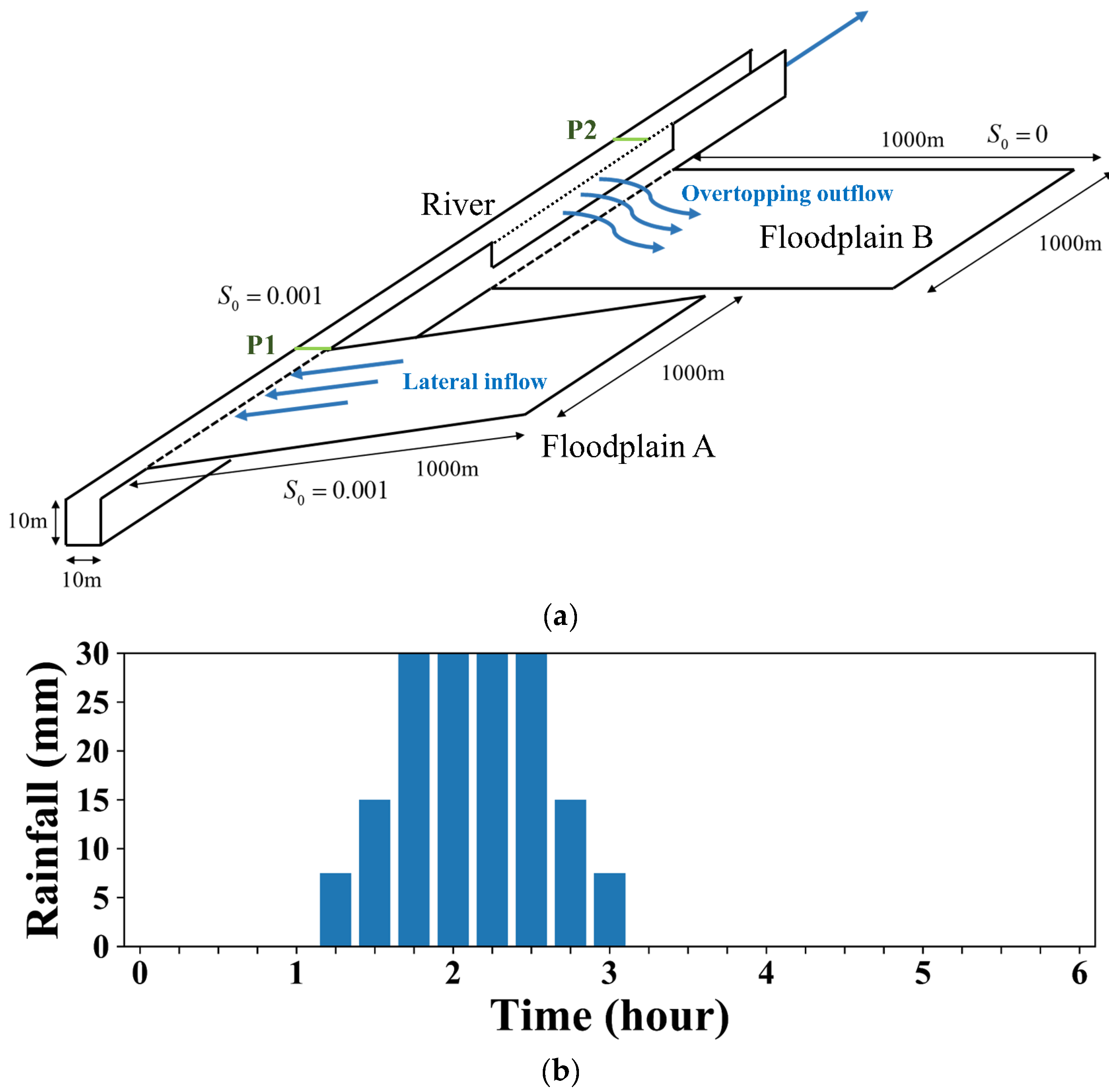
3. Model Verification
3.1. Case Delineation
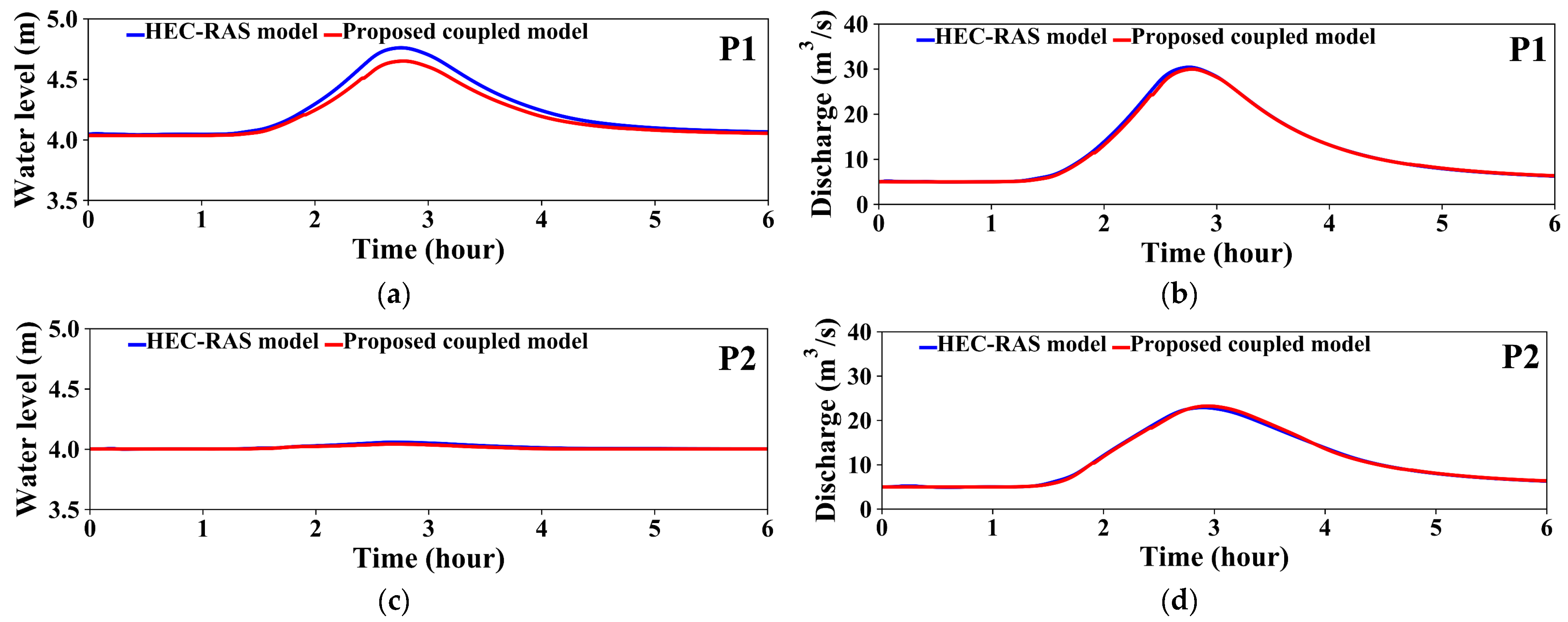
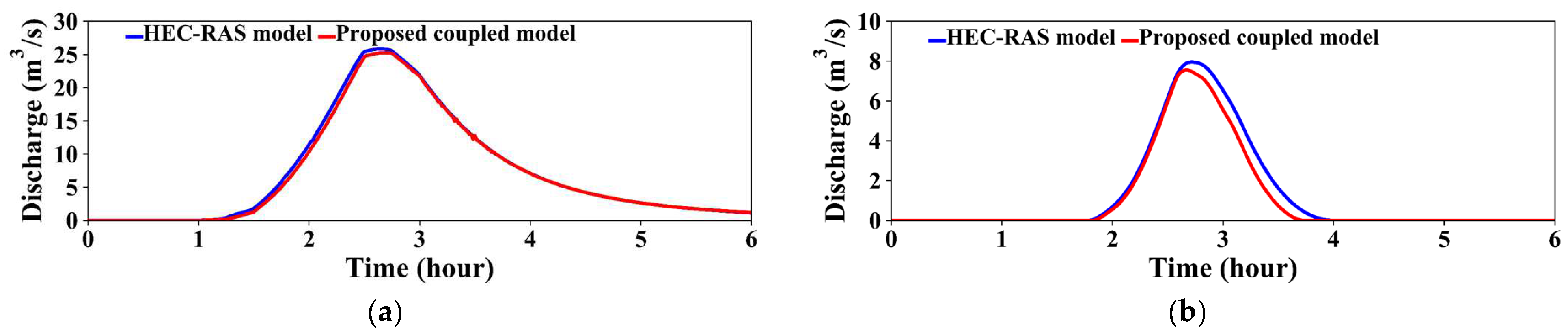
3.2. Accuracy Verification and Efficiency Assessment
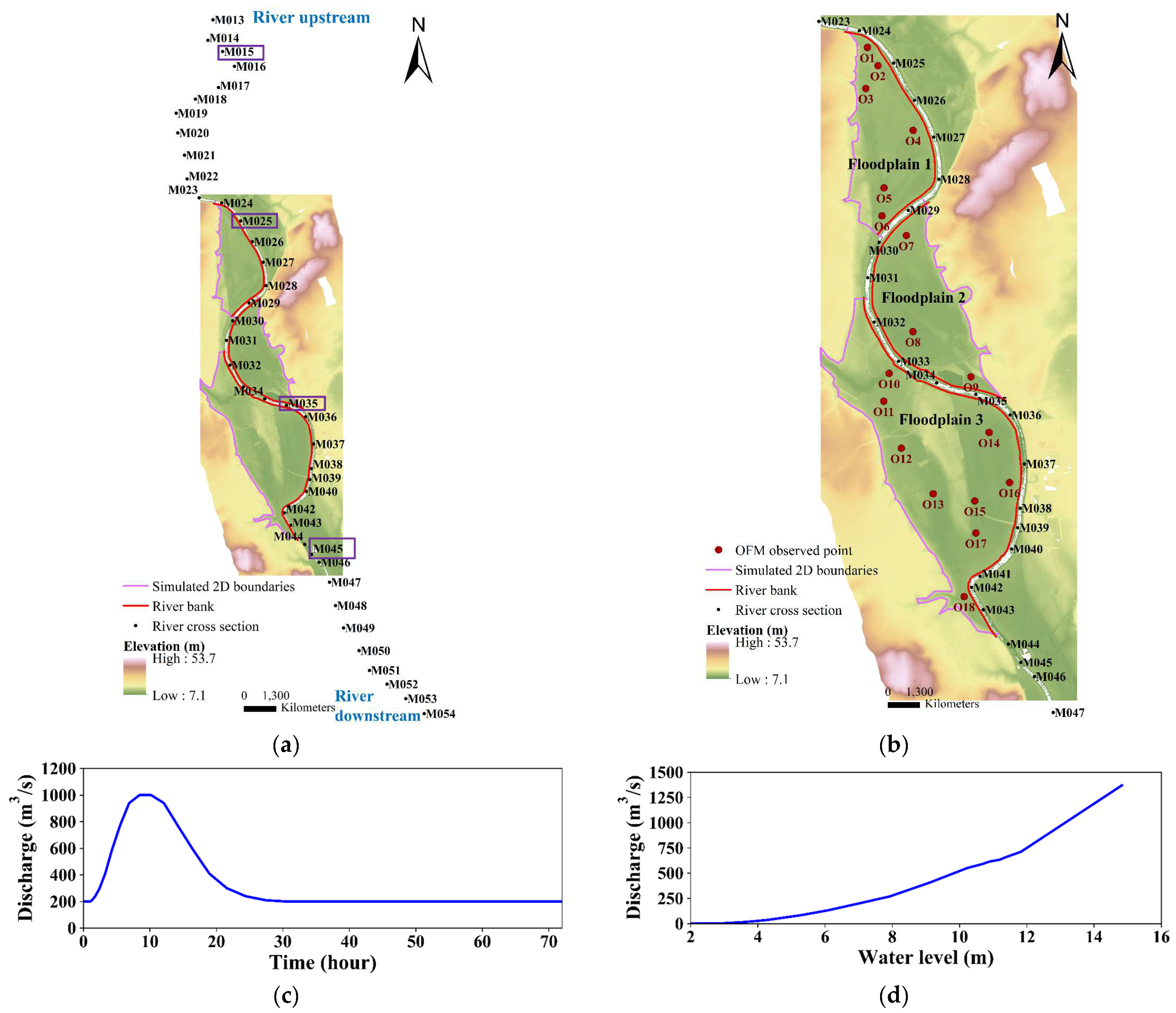
4. Model Applications
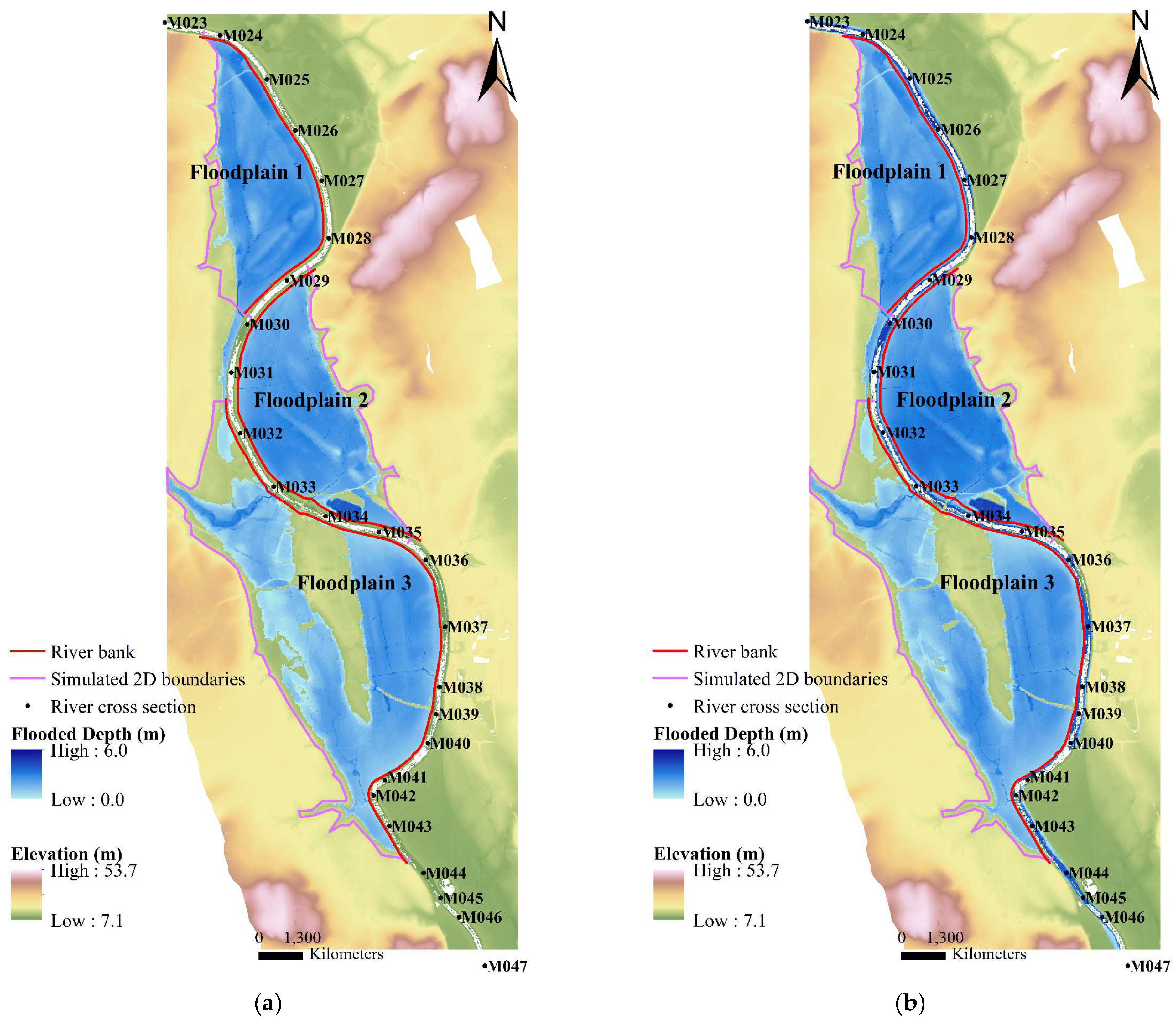
4.1. Study Site Delineation
4.2. Accuracy Evaluation and Efficiency Assessment
5. Conclusions
Author Contributions
Funding
Data Availability Statement
Acknowledgments
Conflicts of Interest
References
- Castro-Orgaz, O.; Hager, W.H. Shallow Water Hydraulics; Springer: Cham, Switzerland, 2019. [Google Scholar]
- Verwey, A. Latest development in floodplain modelling-1D/2D integration. In Proceedings of the Australian Conference on Hydraulics in Civil Engineering, the Institute of Engineers, Hobart, Australia, 20–30 November 2001; pp. 13–24. [Google Scholar]
- Lin, B.; Wicks, J.M.; Falconer, R.A.; Adams, K. Integrating 1D and 2D hydrodynamic models for flood simulation. Proc. Inst. Civ. Eng.-Water Manag. 2006, 159, 19–25. [Google Scholar] [CrossRef]
- Kuiry, S.N.; Sen, D.; Bates, P.D. Coupled 1D-quasi 2D flood inundation model with unstructured grids. J. Hydraul. Eng. 2010, 136, 493–506. [Google Scholar] [CrossRef]
- Masoero, A.; Claps, P.; Asselman, N.E.M.; Mosselman, E.; Di Baldassarre, G. Reconstruction and analysis of the Po River inundation of 1951. Hydrol. Process. 2013, 27, 1341–1348. [Google Scholar] [CrossRef]
- Néelz, S.; Pender, G. Benchmarking the Latest Generation of 2D Hydraulic Modelling Packages; U.K. Environment Agency: Bristol, UK, 2013.
- Liang, D.; Falconer, R.A.; Lin, B. Linking one- and two-dimensional models for free surface flows. Water Manag. 2007, 160, 145–151. [Google Scholar] [CrossRef]
- Morales-Hernánez, M.; Petacciab, G.; Brufaua, P.; García-Navarroa, P. Conservative 1D-2D coupled numerical strategies applied to river flooding: The Tiber (Rome). Appl. Math. Model. 2016, 40, 2087–2105. [Google Scholar] [CrossRef]
- Liu, Q.; Qin, Y.; Zhang, Y.; Li, Z. A coupled 1D-2D hydrodynamic model for flood simulation in flood detention basin. Nat. Hazards 2015, 75, 1303–1325. [Google Scholar] [CrossRef]
- Brunner, G.W. HEC-RAS River Analysis System, Hydraulic Reference Manual; U.S. Army Corps of Engineers Institute for Water Resources Hydrologic Engineering Center: Washington, DC, USA, 2016.
- Innovyze. Inforwork ICM Help, version v3.0; Innovyze: Portland, OR, USA, 2012. [Google Scholar]
- Hénonin, J.; Ma, H.; Yang, Z.Y.; Hartnack, J.; HavnØ, K.; Gourbesville, P.; Mark, O. Citywide multi-grid urban flood modelling: The July 2012 flood in Beijing. Urban Water J. 2013, 12, 52–66. [Google Scholar] [CrossRef]
- Chaudhry, M.H. Open-Channel Flow, 3rd ed.; Springer: New York, NY, USA, 2022. [Google Scholar]
- Lee, M.E.; Seo, I.W. Analysis of pollutant transport in the Han River with tidal current using a 2D finite element model. J. Hydro-Environ. Res. 2007, 1, 30–42. [Google Scholar] [CrossRef]
- Bates, P.D.; Horritt, M.S.; Fewtrell, T.J. A simple inertia formulation of the shallow water equations for efficient two-dimensional flood inundation modeling. J. Hydrol. 2010, 387, 33–45. [Google Scholar] [CrossRef]
- Kao, H.M.; Chang, T.J. Numerical modeling of dambreak-induced flood and inundation using smoothed particle hydrodynamics. J. Hydrol. 2012, 448–449, 232–244. [Google Scholar] [CrossRef]
- Chang, T.J.; Wang, C.H.; Chen, A.S. A novel approach to model dynamic flow interactions between storm sewer system and overland surface for different land covers in urban areas. J. Hydrol. 2015, 524, 662–679. [Google Scholar] [CrossRef]
- Ferrari, A.; Vacondio, R.; Dazzi, S.; Mignosa, P. A 1D-2D Shallow Water Equations solver for discontinuous porosity field based on a Generalized Riemann Problem. Adv. Water Resour. 2017, 107, 233–249. [Google Scholar] [CrossRef]
- Martins, R.; Leandro, J.; Djordjević, S. Wetting and drying numerical treatments for the Roe Riemann scheme. J. Hydraul. Res. 2018, 56, 256–267. [Google Scholar] [CrossRef]
- Yu, H.L.; Chang, T.J. A hybrid shallow water solver for overland flow modelling in rural and urban areas. J. Hydrol. 2021, 598, 126262. [Google Scholar] [CrossRef]
- Zhao, J.; Liang, Q. Novel variable reconstruction and friction term discretization schemes for hydrodynamic modelling of overland flow and surface water flooding. Adv. Water Resour. 2022, 163, 104187. [Google Scholar] [CrossRef]
- Xia, X.; Liang, Q.; Ming, X.; Hou, J. An efficient and stable hydrodynamic model with novel source term discretization schemes for overland flow and flood simulations. Water Resour. Res. 2017, 53, 3730–3759. [Google Scholar] [CrossRef]
- Muthusamy, M.; Casado, M.R.; Butler, D.; Leinster, P. Understanding the effects of Digital Elevation Model resolution in urban fluvial flood modelling. J. Hydrol. 2021, 596, 126088. [Google Scholar] [CrossRef]
- Chang, T.J.; Yu, H.L.; Wang, C.H.; Chen, A.S. Dynamic-wave cellular automata framework for shallow water flow modeling. J. Hydrol. 2022, 613, 128449. [Google Scholar] [CrossRef]
- Jamali, B.; Löwe, R.; Bach, P.M.; Urich, C.; Arnbjerg-Nielsen, K.; Deletic, A. A rapid urban flood inundation and damage assessment model. J. Hydrol. 2018, 564, 1085–1098. [Google Scholar] [CrossRef]
- Savage, J.T.S.; Bates, P.; Freer, J.; Neal, J.; Aronica, G. When does spatial resolution become spurious in probabilistic flood inundation predictions? Hydrol. Process. 2016, 30, 2014–2032. [Google Scholar] [CrossRef]
- Vacondio, R.; Dal Palù, A.; Mignosa, P. GPU-enhanced finite volume shallow water solver for fast flood simulations. Environ. Modell. Softw. 2014, 57, 60–75. [Google Scholar] [CrossRef]
- Leandro, J.; Chen, A.S.; Schumann, A. A 2D parallel diffusive wave model for floodplain inundation with variable time step (P-DWave). J. Hydrol. 2014, 517, 250–259. [Google Scholar] [CrossRef]
- Caviedes-Voullième, D.; Fernández-Pato, J.; Hinz, C. Performance assessment of 2D zero-inertia and shallow water models for simulating rainfall-runoff process. J. Hydrol. 2020, 584, 124663. [Google Scholar] [CrossRef]
- Krupka, M. A Rapid Inundation Flood Cell Model for Flood Risk Analysis. Ph.D. Thesis, Heriot-Watt University, Edinburgh, Scotland, 2009. [Google Scholar]
- Bernini, A.; Franchini, M. A rapid model for delimiting flooded areas. Water Resour. Manag. 2013, 27, 3825–3846. [Google Scholar] [CrossRef]
- Maksimović, Č.; Prodanovic, D.; Boonya-aroonnet, S.; Leitäo, J.P.; Djordjević, S.; Allitt, R. Overland flow and pathway analysis for modelling of urban pluvial flooding. J. Hydraul. Res. 2009, 47, 512–523. [Google Scholar] [CrossRef]
- Chopard, B. Cellular automata modeling of physical systems. In Encyclopedia of Complexity and Systems Science, 1st ed.; Meyers, R.A., Ed.; Springer: New York, NY, USA, 2009; pp. 856–892. [Google Scholar]
- Hadeler, K.P.; Müller, J. Cellular Automata: Analysis and Applications; Springer: Cham, Switzerland, 2017. [Google Scholar]
- Wolfram, S. Cellular automata as models of complexity. Nature 1984, 311, 419–424. [Google Scholar] [CrossRef]
- Yu, H.L.; Chang, T.J. Modeling particulate matter concentration in indoor environment with cellular automata framework. Build Environ. 2022, 214, 108898. [Google Scholar] [CrossRef]
- Dottori, F.; Todini, E. Developments of a flood inundation model based on the cellular automata approach: Testing different methods to improve model performance. Phys. Chem. Earth Parts ABC 2011, 36, 266–280. [Google Scholar] [CrossRef]
- Ghimire, B.; Chen, A.S.; Guidolin, M.; Keedwell, E.C.; Djordjević, S.; Savić, D.A. Formulation of a fast 2D urban pluvial flood model using a cellular automata approach. J. Hydroinform. 2013, 15, 676. [Google Scholar] [CrossRef]
- Cai, X.; Li, Y.; Wen, G.X.; Wu, W. Mathematical model for flood routing based on cellular automation. Water Sci. Eng. 2014, 7, 133–142. [Google Scholar]
- Guidolin, M.; Chen, A.S.; Ghimire, B.; Keedwell, E.C.; Djordjević, S.; Savić, D.A. A weighted cellular automata 2D inundation model for rapid flood analysis. Environ. Model. Softw. 2016, 84, 378–394. [Google Scholar] [CrossRef]
- Jahanbazi, M.; Özgen, I.; Aleixo, R.; Hinkelmann, R. Development of a diffusive wave shallow water model with a novel stability condition and other new features. J. Hydroinform. 2017, 19, 405–425. [Google Scholar] [CrossRef]
- Jamali, B.; Bach, P.M.; Cunningham, L.; Deletic, A. A cellular automata fast flood evaluation (CA-ffé) model. Water Resour. Res. 2019, 55, 4936–4953. [Google Scholar] [CrossRef]
- Tavakolifar, H.; Abbasizadeh, H.; Nazif, S.; Shahghasemi, E. Development of 1D-2D urban flood simulation model based on modified cellular automata approach. J. Hydrol. Eng. 2020, 26, 2. [Google Scholar] [CrossRef]
- Caviedes-Voullième, D.; Fernández-Pato, J.; Hinz, C. Cellular automata and finite volume solvers converge for 2D shallow flow modeling for hydrological modelling. J. Hydrol. 2018, 563, 411–417. [Google Scholar] [CrossRef]
- Yin, D.; Evans, B.; Wang, Q.; Chen, Z.; Jia, H.; Chen, A.S.; Fu, G.; Ahmad, S.; Leng, L. Integrated 1D and 2D model for better assessing runoff quantity control of low impact development facilities on community scale. Sci. Total Environ. 2020, 720, 137630. [Google Scholar] [CrossRef] [PubMed]
- Chang, T.J.; Yu, H.L.; Wang, C.H.; Chen, A.S. Overland-gully-sewer (2D-1D-1D) urban inundation modeling based on cellular automata framework. J. Hydrol. 2021, 603, 127001. [Google Scholar] [CrossRef]
- Hsu, M.H.; Lin, S.H.; Fu, J.C.; Chung, S.F.; Chen, A.S. Longitudinal stage profiles forecasting in rivers for flash floods. J. Hydrol. 2010, 388, 426–437. [Google Scholar] [CrossRef]
- Hunter, N.M.; Horritt, M.S.; Bates, P.D.; Wilson, M.D.; Wener, M.G.F. An adaptive time step solution for raster-based storage cell modelling of floodplain inundation. Adv. Water Resour. 2005, 28, 975–991. [Google Scholar] [CrossRef]
- Casulli, V. A high-resolution wetting and drying algorithm for free-surface hydrodynamics. Int. J. Numer. Meth. Fl. 2008, 60, 391–408. [Google Scholar] [CrossRef]
- Nash, J.E.; Sutcliffe, J.V. River flow forecasting through conceptual models part I—A discussion of principles. J. Hydrol. 1970, 10, 282–290. [Google Scholar] [CrossRef]


| Measured Station | The NSE Indicator | The MSE Indicator | ||
|---|---|---|---|---|
| Water Level | Water Discharge | Water Level | Water Discharge | |
| P1 | 0.956 | 0.998 | 0.002 | 0.142 |
| P2 | 0.863 | 0.997 | <0.001 | 0.105 |
| Measured Station | The HEC-RAS Model | The Coupled Model | ||
|---|---|---|---|---|
| Water Level Peak (m) | Arrival Time (min) | Water Level Peak (m) | Arrival Time (min) | |
| P1 | 4.76 | 166.0 | 4.65 | 167.0 |
| P2 | 4.06 | 160.0 | 4.04 | 160.0 |
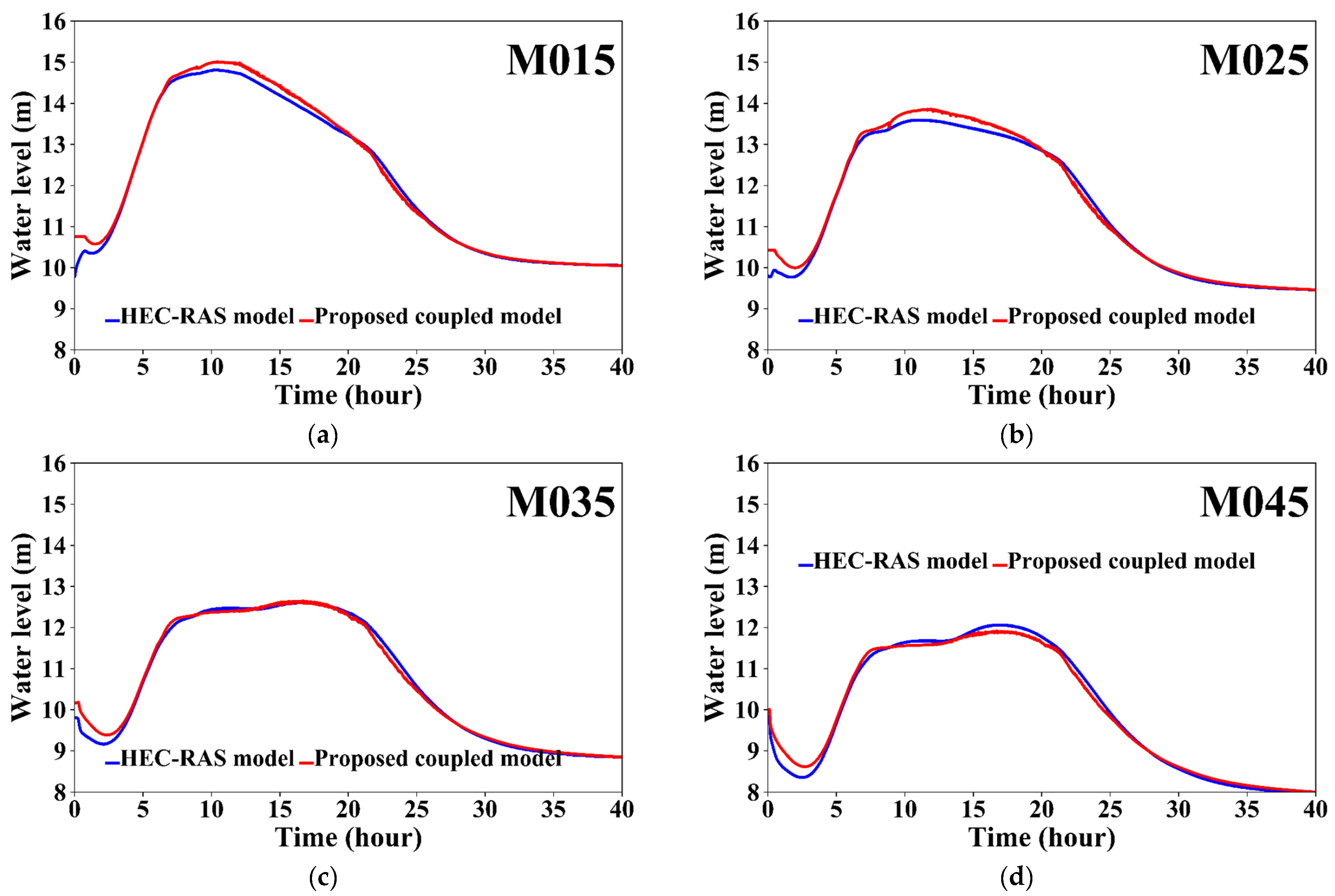
| Cross-Section | The NSE Indicator | The MSE Indicator |
|---|---|---|
| M015 | 0.994 | 0.021 |
| M025 | 0.991 | 0.024 |
| M035 | 0.994 | 0.013 |
| M045 | 0.993 | 0.018 |
| Cross-Section | The HEC-RAS Model | The Coupled Model | ||
|---|---|---|---|---|
| Water Level Peak (m) | Arrival Time (h) | Water Level Peak (m) | Arrival Time (h) | |
| M015 | 14.81 | 10.13 | 15.01 | 10.42 |
| M025 | 13.59 | 10.62 | 13.86 | 11.90 |
| M035 | 12.61 | 16.35 | 12.65 | 16.67 |
| M045 | 12.06 | 16.45 | 11.92 | 16.75 |
| Observed Point | The NSE Indicator | The MSE Indicator |
|---|---|---|
| O1 | 0.943 | 0.029 |
| O2 | 0.928 | 0.053 |
| O6 | 0.978 | 0.015 |
| O8 | 0.976 | 0.025 |
| O9 | 0.952 | 0.031 |
| O11 | 0.818 | 0.074 |
| O12 | 0.914 | 0.011 |
| O14 | 0.982 | 0.011 |
| O17 | 0.990 | 0.008 |
| Observed Point | The HEC-RAS Model | The Coupled Model | ||
|---|---|---|---|---|
| Water Level Peak (m) | Arrival Time (h) | Water Level Peak (m) | Arrival Time (h) | |
| O1 | 13.57 | 10.95 | 13.94 | 11.93 |
| O2 | 13.53 | 11.07 | 13.89 | 11.92 |
| O6 | 13.47 | 11.10 | 13.30 | 12.72 |
| O8 | 12.80 | 15.62 | 12.93 | 15.68 |
| O9 | 12.74 | 15.53 | 12.75 | 16.20 |
| O11 | 12.74 | 15.77 | 12.77 | 16.88 |
| O12 | 12.43 | 16.87 | 12.32 | 17.45 |
| O14 | 12.52 | 16.88 | 12.52 | 16.37 |
| O17 | 12.43 | 16.95 | 12.25 | 17.45 |
Disclaimer/Publisher’s Note: The statements, opinions and data contained in all publications are solely those of the individual author(s) and contributor(s) and not of MDPI and/or the editor(s). MDPI and/or the editor(s) disclaim responsibility for any injury to people or property resulting from any ideas, methods, instructions or products referred to in the content. |
© 2024 by the authors. Licensee MDPI, Basel, Switzerland. This article is an open access article distributed under the terms and conditions of the Creative Commons Attribution (CC BY) license (https://creativecommons.org/licenses/by/4.0/).
Share and Cite
Yu, H.-L.; Chang, T.-J.; Wang, C.-H.; Maa, S.-Y. A Coupled River–Overland (1D-2D) Model for Fluvial Flooding Assessment with Cellular Automata. Water 2024, 16, 2703. https://doi.org/10.3390/w16182703
Yu H-L, Chang T-J, Wang C-H, Maa S-Y. A Coupled River–Overland (1D-2D) Model for Fluvial Flooding Assessment with Cellular Automata. Water. 2024; 16(18):2703. https://doi.org/10.3390/w16182703
Chicago/Turabian StyleYu, Hsiang-Lin, Tsang-Jung Chang, Chia-Ho Wang, and Shyh-Yuan Maa. 2024. "A Coupled River–Overland (1D-2D) Model for Fluvial Flooding Assessment with Cellular Automata" Water 16, no. 18: 2703. https://doi.org/10.3390/w16182703