Article

A Methodology for the Prediction of Extreme Precipitation in Complex Terrains: A Case Study of Central Southwest China

1
Carbon Neutral Innovation Research Center, Xiamen University, Xiamen 361102, China
2
Polar and Marine Research Institute, College of Harbor and Coastal Engineering, Jimei University, Xiamen 361021, China
3
Key Laboratory of Physical Oceanography, Ocean University of China, Qingdao 266100, China
4
State Key Laboratory of Marine Environmental Science and College of Ocean and Earth Sciences, Xiamen University, Xiamen 361102, China
5
Fujian Provincial Key Laboratory of Disaster Weather, Fuzhou 350000, China
6
Meteorological Administration of Zhangzhou in China, Zhangzhou 363600, China
*
Authors to whom correspondence should be addressed.
These authors contributed equally to this work.
Water 2024, 16(3), 427; https://doi.org/10.3390/w16030427
Submission received: 19 December 2023 / Revised: 12 January 2024 / Accepted: 16 January 2024 / Published: 28 January 2024

Abstract

:
Against the backdrop of global warming, extreme precipitation events have become more frequent. In complex terrain regions, due to the vulnerability of their ecosystems, extreme precipitation events can lead to significant secondary disasters. Utilizing daily rainfall data from the National Meteorological Information Center of China and statistical analysis, this study explores the spatial and temporal distribution of extreme precipitation in the Central Southwest China (CSC) region. The temporal pattern of extreme precipitation in CSC shows a consistent trend, while the spatial distribution reveals an opposite phase between the northern and southern parts of CSC. Based on this, we propose a new method for constructing extreme precipitation prediction models for complex terrain regions based on physical mechanisms, and take CSC area as a study case. Instead of anonymous feature selection, this method improves the accuracy and stability of the model by studying the impact of sea–air interactions on extreme precipitation and then introducing it into deep learning. It was found that the sea surface temperature (SST) anomaly in the South Indian Ocean affects extreme precipitation in the CSC by influencing uplift, atmospheric instability, and moisture. The SST anomaly also affects the intensity of cross-equatorial airflow, which changes the trajectory of the Pacific–Japan teleconnection wave and impacts extreme precipitation. These findings provide a comprehensive and reliable approach for forecasting extreme precipitation in CSC and are further integrated into the extreme precipitation prediction models.

1. Introduction

Influenced by human activities and the industrial revolution, greenhouse gas emissions are increasing rapidly, and the IPCC [1] points out that global warming is a foregone conclusion. Rising temperatures are likely to cause changes in extreme climate events, which also have a negative impact on human society and the environment. Therefore, extreme climate events, especially extreme precipitation events, have attracted global attention. Understanding the mechanism of extreme precipitation is essential for predicting flood events and preventing secondary disasters caused by floods [2,3,4,5].
Recently, deep learning methods have been widely used in the prediction of extreme precipitation events, and SST (sea surface temperature) plays an important role in these predictions (e.g., [6,7,8,9]). However, in these studies, researchers often did not delve into the physical mechanisms between SST and extreme precipitation. They only used statistical analysis methods to select the best feature combinations from numerous features. This can lead to significant increases in the instability of the models [8,9]. The physical mechanism of SST’s impact on precipitation can be attributed to several factors [8,9]. First, increased SST leads to higher evaporation rates, consequently elevating atmospheric water vapor content. This increased moisture in the atmosphere contributes to greater precipitation [10].
Secondly, elevated SSTs can intensify convective activities by providing additional heat and energy to the atmosphere, resulting in more vigorous convection and, consequently, increased precipitation intensity and frequency [11]. Additionally, SST changes can influence tropical circulation patterns, such as the subtropical high-pressure system and monsoonal circulations, thus altering precipitation distribution. Lastly, SST variations affect the interactions between the ocean and the atmosphere, with higher SSTs enhancing evaporation rates and releasing more moisture into the atmosphere. This influx of moisture subsequently alters the atmospheric thermodynamic and moisture conditions, ultimately impacting the occurrence and distribution of precipitation. In summary, the impact of SST on precipitation operates through regulating atmospheric water vapor content, promoting convective activities, modifying circulation systems, and influencing ocean–atmosphere interactions. These mechanisms collectively determine the extent and patterns of SSTs’ influence on precipitation [8,9], thus clarifying that the mechanism of the influence of SST on precipitation can further improve the prediction results in deep learning methods.
Located southeast of the Tibetan Plateau, the Central Southwest China (CSC) region is characterized by a mountainous and complex terrain with an average elevation of 1500 m above sea level, featuring an elevation range of 100–4000 m. Such topographical complexity often amplifies the effects of the most extreme convective rainfall events, leading to frequent landslides and flash floods (e.g., [12,13]). Due to its overpopulation, underdevelopment, and vulnerable ecosystems [11,13], the CSC region shows both sensitivity and vulnerability to the potential effects of climate change. Various studies have documented heterogeneous trends in extreme precipitation over CSC between 1959 and 2022, with decreasing spatial variability [12,13]. Some studies [14,15] found that the changes in extreme precipitation were relatively small during 1961–2008. Xiao et al. [16] detected an increasing trend in extreme precipitation in CSC between 1971 and 2013; therefore, predicting extreme precipitation in this region has become a research hot topic [17,18].
As we know, extreme precipitation processes are rather complex and difficult to characterize in CSC (e.g., [12,13]). The extreme precipitation prediction can have significant practical implications for disaster preparedness and mitigation strategies [19]. By providing early warning of potential flood events, informing infrastructure planning and design, and aiding in disaster response and recovery efforts, extreme precipitation prediction can help reduce the risk and impact of flooding on communities and infrastructure ([18] and its references). However, extreme precipitation processes in CSC pose a challenge due to their complex nature, making characterization difficult [12,13,18]. The prediction of climate in CSC is especially challenging, despite efforts to improve seasonal predictions through dynamic models. For example, dynamic models still struggle to capture the interannual variability of CSC precipitation, leading to unsatisfactory dynamical prediction skills for extreme precipitation [20]. A promising alternative is to establish a machine learning-based algorithm that leverages the physical relationship between predictands and climate features. This approach has shown success in predicting seasonal precipitation or extreme precipitation in other regions such as Pakistan [21], South China [22], and Northeast China [23]. However, little research has focused on the statistical prediction of summer extreme precipitation in CSC.
Therefore, we have selected this region as the study area to explore how to scientifically construct extreme precipitation prediction models for complex terrain regions based on physical mechanisms. Section 2 describes the dataset and the methods used in this paper. Section 3 shows the temporal and spatial distribution characteristics of summer extreme precipitation in CSC. Section 3 describes the selection of key areas of SST affecting CSC extreme precipitation and the analysis of the physical mechanisms is also explained in Section 4. Section 5 summarizes the conclusions.

2. Data and Method

2.1. Data

The daily precipitation data (the spatial distribution of stations shown in Figure 1) from 2000 to 2018 for the CSC were downloaded from a dataset of 2480 stations across China provided by the National Meteorological Information Center, China Meteorological Administration. This dataset was subjected to rigorous quality control, and stations were removed when their missing value rate exceeded 5%. Quality control measures of precipitation data are used to ensure that the data collected are accurate and reliable. In accordance with Jan et al. [24], we used the following quality control measures, implemented to ensure the accuracy of the collected data: (1) Visual Inspection: This is the most basic quality control measure, where the data are inspected visually to identify any errors or inconsistencies; (2) Statistical Analysis: Statistical methods are used to detect outliers, errors, and inconsistencies in the data. Common statistical tests include checking for normality, skewness, kurtosis, and outliers; (3) Duplicate Checking: Duplicate checking involves comparing the precipitation data with data from other nearby stations. If there are discrepancies between the two sets of data, it can indicate an error in one of the datasets; (4) Consistency Checks: Consistency checks are used to verify that the data are consistent over time. For example, the data should not change abruptly from one period to another without any explanation; (5) Calibration: Calibration is used to ensure that the equipment used to collect the precipitation data is accurate and reliable. Regular calibration is necessary to maintain the accuracy of the data.
The summer average refers to the average of June–August of the current year, and the average of 2000–2018 was calculated as the climate mean. And we also gridded these station-based observation data into 0.25° × 0.25°.
The monthly mean atmospheric circulation, wind, and outgoing long-wave radiation (OLR) were obtained from the NCEP/NCAR reanalysis datasets (https://psl.noaa.gov/data/reanalysis/reanalysis.shtml, accessed on 12 July 2020). These datasets consist of high-quality, gridded global atmospheric fields at standard pressure levels, with a vertical resolution of 17 levels, covering the same period under investigation [25]. In addition, the monthly SST from NOAA’s Optimum Interpolation Sea Surface Temperature (OISST, also known as Reynolds’ SST) is a series of global analysis products on a 2° (longitude) × 1° (latitude) grid [26].

2.2. Method

This study presents a new method to scientifically construct extreme precipitation prediction models for complex terrain regions based on physical mechanisms. The entire method is divided into four steps: (1) analyze the spatial and temporal distribution characteristics of extreme precipitation in the study area, the CSC; (2) perform lead–lag correlation analysis between the time series of extreme precipitation index and global SST changes (with SST time series leading extreme precipitation index by 6 months, 3 months, 1 month, and in-phase) and select the key sea areas of SST that affect the precipitation in the study area; (3) study the physical mechanisms of abnormal precipitation in the SST impact area using earth science data (such as geopotential height and wind field data); (4) incorporate the above physical mechanisms into deep learning methods (CNN-LSTM, details can be found in Section 2.2.3 and Section 2.2.4) and compare the effects of different feature selections on the results. This research method avoids blind features selection and improves the accuracy and stability of prediction models. Details are as follows:

2.2.1. Extreme Precipitation Index

One of the WMO-CCl/CLIVAR Working Groups aimed to identify extreme climate indices and completed a climate extreme analysis on all parts of the world where appropriate data were available for climate change detection [27]. We chose the R95 index from these extreme climate indices because this index has become one of the core indices recommended by the Strdex-plan to describe extreme precipitation events [24]. The R95 index represents precipitation in a specific day over 95% of historical daily precipitation, calculated as follows.
The daily precipitation records of the site are arranged in ascending order, and the value of extreme precipitation index x is as follows:
x = (1 − a) × j + a × x j + 1
In Formula (1), j represents the ordinal number,
j = int[p × (n + 1)]
In Formula (2), Int is an integer function, p is the percentile, and n stands for the total observational times. In this paper, the value of p is 95% and a stands for the weight coefficient.
A = p ×(n + 1) − j

2.2.2. Statistical Analysis

The wavelet power spectrum reflects the intensity of periodic signals of different scales, which can reveal the internal frequency structure of the signal sequences and can give a complete description of the relative contribution of varying scale oscillations contained in the sequences [28]. The wavelet power spectrum and the global wavelet power spectrum are complementary tools that can be used together to gain a better understanding of the behavior of time-varying signals. The wavelet power spectrum represents the power of a signal at different frequency scales and time intervals, while the global wavelet power spectrum represents the spatial average of the wavelet power spectrum over a specific region. While the wavelet power spectrum provides a detailed view of the frequency content of the signal over time, the global wavelet power spectrum provides a broader picture of the spatial distribution of this variability.
The EOF (empirical orthogonal function) method was established in 1902 [29]. It decomposes elements of a set of space–time data into two parts, one dependent only on time, and another dependent only on space to analyze the spatial structure of the element field [30]. Thus, EOF decomposition is commonly used to analyze spatial and temporal variations in meteorological elements. Singular value decomposition (SVD) [31,32] is usually applied to two data fields together to identify pairs of coupled spatial patterns, which explains, as much as possible, the covariance between the two variables. In addition, we also use a t-test to ensure the reliability of the conclusion.
In this study, we used wavelet method on the station-based precipitation data to obtain its periodic signals, and used the EOF method on the gridded station-based precipitation data to analyze its spatial and temporal variations, and used the SVD method on the gridded station-based precipitation data and SST data to identify pairs of coupled spatial patterns.

2.2.3. Convolutional Neural Network

The initial purpose of developing the convolutional neural network (CNN) was for object recognition in digital image processing [33]. This network is structured with a convolution layer, pooling layer, and fully connected layers. The convolution layer applies a convolution filter to input two-dimensional data, resulting in a feature map. These feature maps, generated through different filters, are then combined to produce the final output. Typically, an activation function, often the rectified linear unit (ReLU), is applied in the convolutional layer to enhance non-linear signals [34].
Subsequent to the convolution layer, the max-pooling layer is used to extract invariant features by discarding non-maximal values, achieving non-linear downsampling with an efficient convergence rate [35]. The fully connected layer, linked to the max-pooling layer, connects a loss function to calculate errors between observed values and model outputs [36]. In this particular study, the root mean squared error (RMSE) is chosen as the loss function.

2.2.4. Long Short-Term Memory

The LSTM network, a type of recurrent neural network (RNN), employs a cyclic structure that transfers the hidden layer’s output back to itself, allowing it to capture temporal features and information from previous time series signals [37]. Proposed by Hochreiter and Schmidhuber [38], LSTM was designed to address the vanishing gradient problem through the use of memory cells [21]. These cells are updated using gated mechanisms involving three specific gates: the input gate determines the information to be updated in the current state and which new data should be included as inputs; the forget gate controls the retention or discarding of information; and the output gate governs the generation of outputs [39].
The CNN-LSTM model has high computational requirements which can pose challenges when implementing the model in practice [40]. In this study, to address this challenges, we used the optimizing hyperparameters method and used regularization techniques. These methods can help to balance the trade-off between model complexity and computational efficiency, enabling the CNN-LSTM model to be implemented more effectively.

2.2.5. Loss Function

Moreover, it is necessary to evaluate the accuracy of any algorithm based on certain error metrics before applying it to specific scenarios. The mean squared error (MSE) represents the standard deviation of the residuals (prediction error), where the residuals represent the distance between the fitted line and the data point, i.e., the degree of concentration of the reconstructed data around the regression line. In regression analysis, the RMSE is commonly used to verify experimental results. To assess bias, the RMSE needs to combine the magnitude of the model data and is calculated as follows:
R M S E = 1 n i = 1 n ( y i y r i ) 2
where y stands for the in situ data, yr represents the reconstructed data, and n is the number of data. The root mean squared error (RMSE) is a commonly used loss function in various machine learning tasks, including regression problems [41]. It is often chosen as the loss function for the CNN-LSTM model due to several reasons: (1) RMSE penalizes large errors more compared with other loss functions such as mean absolute error (MAE). This makes it suitable for datasets that may contain outliers or extreme values. By considering the squared errors, RMSE provides a higher emphasis on significant deviations from the predicted values; (2) RMSE is a differentiable function, which means it has a smooth gradient that can be computed efficiently during the backpropagation process. This property is crucial for optimizing the model parameters using gradient-based optimization algorithms like stochastic gradient descent (SGD) or Adam; (3) RMSE is the square root of the average of squared differences between predicted and actual values. It represents the Euclidean distance between the predicted and actual values in the feature space. This interpretation is intuitive and aligns with the concept of minimizing the overall distance between predictions and ground truth; (4) Minimizing RMSE inherently promotes accurate predictions. Since RMSE squares the errors, larger errors are amplified, pushing the model to focus more on reducing those errors. This property is valuable when the goal is to prioritize accurate predictions over slight deviations [41].

3. Results

3.1. The Spatial and Temporal Distribution of Extreme Precipitation in CSC

As shown in Figure 1, the CSC has complex topography features. The height of the terrain in the CSC increases from northwest to southeast. However, the air automatic monitoring stations here are densely distributed, hence the data records have high reliability.
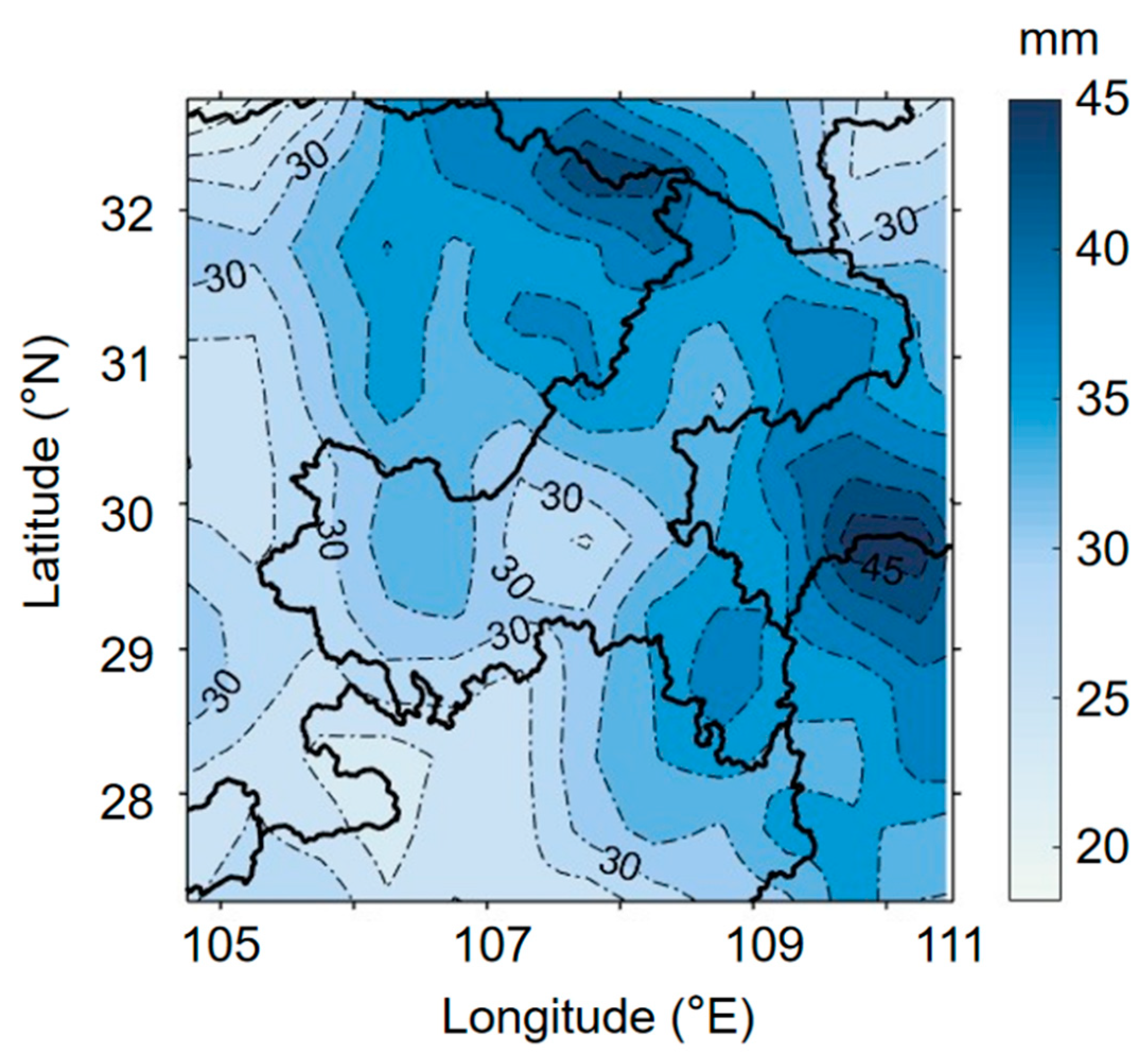
Extreme precipitations have regional characteristics (e.g., [15,16]). To perform spatial analysis for the extreme precipitation distribution, we calculated the R95 extreme precipitation index of each station in the CSC in summer (Figure 2). The extreme precipitation distribution in the CSC showed an apparent large gradient (Figure 2), and it coincided, to a certain extent, with the contour line of topography in Figure 1. The R95 index decreased from the upwind slope in the southeast to the basin on the west side. This distribution showed that the extreme precipitation in the CSC may be affected by the uplift caused by the topography.
By analyzing empirical orthogonal function (EOF) decomposition, we further explored the temporal and spatial distribution of the summer extreme precipitation frequency in the CSC. From the table of the variance contribution rate (Table 1), the total variance contribution of the first two modes is more than 60%, and the variance contribution of the third mode is much lower; the first two modes describe the spatial distribution of extreme precipitation frequency in summer over the CSC quite well.
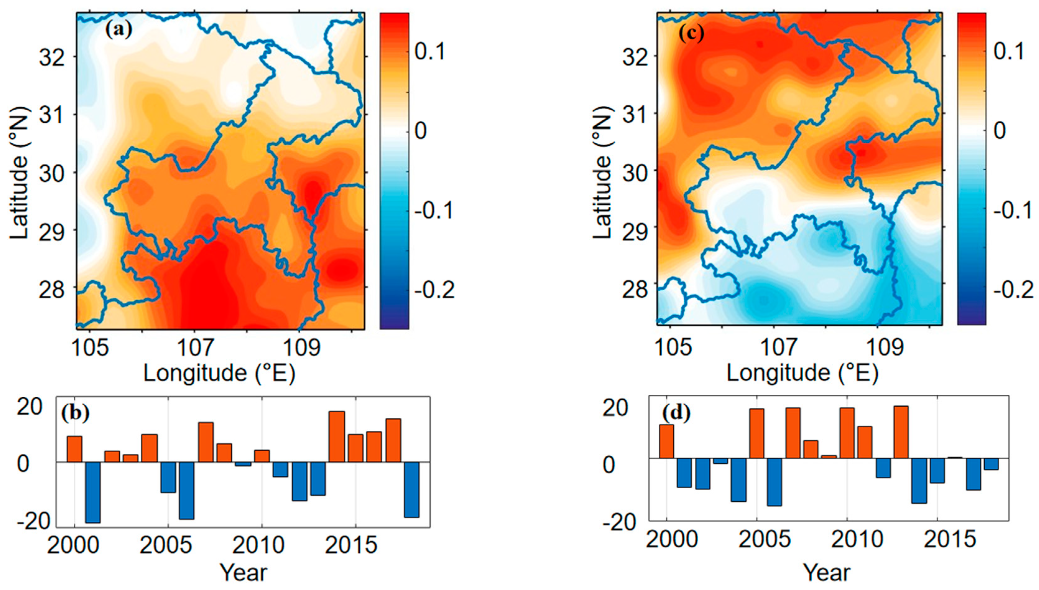
Figure 3 showed the spatial patterns of the two leading EOFs of summer extreme precipitation variability in the CSC, obtained by the linear regression of extreme precipitation frequency on the respective principal component time series. The first EOF mode of the summer extreme precipitation frequency was consistently positive with a variance contribution of 40.12%, and the value of the southeast was higher than that of the northwest (Figure 3a). This means that the trend of extreme precipitation frequency in the CSC has a solid spatial consistency, which is likely contributed by the influence of large-scale weather systems. For the time series of the first EOF mode (Figure 3b), the occurrence times of positive values were higher than those of negative values, indicating that the extreme precipitation frequency fluctuated wildly in the CSC, which makes extreme precipitation challenging to forecast.
The spatial distribution of the second EOF mode (Figure 3c) showed obvious north–south reversed phases. The time series (Figure 3d) fluctuated greatly, resulting from the large latitude span of the rain belt. In the classification proposed by Wu et al. [12], the CSC is located in the control area of both the northern and southern rain belt. When the rain belt is more northern than the climatological states, extreme precipitation is prone to occur in the north CSC, and when the rain belt is southward, the extreme precipitation frequency in the south increases. The spatiotemporal distribution of China’s rain belt may also be affected by the ocean. The movement of the rain belt is owed to the change in the subtropical high intensity [12], on which the impact of the SST anomaly cannot be ignored [42,43]. Thus, the extreme precipitation frequency in the CSC is closely related to the SST.
To better explore the periodic signal variation in summer extreme precipitation from 2000 to 2018 in the CSC, we calculated the wavelet power spectrum of the summer extreme precipitation frequency (the occurring times of the extreme precipitation (exceeded the R95 index) from the atmospheric automatic monitoring stations records during each summer of 2000–2018). As shown in Figure 4, overall, the periodic signals of summer extreme precipitation showed a complex periodic situation with multiple time scales nesting in each other. It not only has a main precipitation period of approximately 1.5 years but also a notable subperiod of approximately 3–4 years. Both of these showed negative phases, indicating that, against the background of global warming, the extreme precipitation frequency in the CSC has tended to increase from the beginning of the 21st century. By conducting wavelet analysis on summer extreme precipitation from 2000 to 2018 in the CSC, we found the presence of multi-scale and multi-period nested variations in precipitation in the region. This finding simultaneously demonstrates the significant challenge in accurately predicting extreme precipitation in this area.
Thus, the extreme precipitation index and variation form of its frequency in the CSC were complex and diverse; at the same time, the time series showed a periodically increasing gradual trend. Since the 21st century, the frequency of extreme climate events has increased because of the changes in SST under global warming (IPCC, 1). As a significant forcing factor in the atmosphere changes, SST anomalies indirectly lead to the abnormal distribution of extreme precipitation. Therefore, it is necessary to analyze the relations between SST and extreme precipitation frequency in the CSC to improve the predicting ability of extreme precipitation.

3.2. The Predict Model of Extreme Precipitation Frequency in Summer for the CSC

3.2.1. The Key Areas of SST Affect

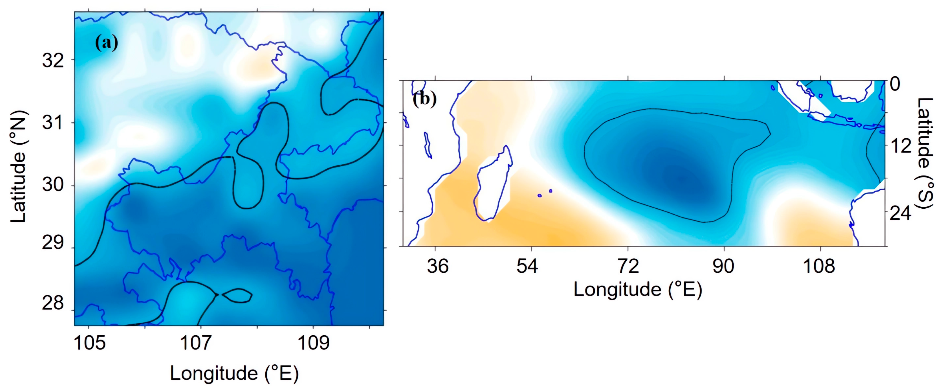
By using the lead–lag correlation analysis, we found that the SST of the South Indian Ocean shows a relatively large correlation coefficent (0.69, passing the 95% t-test) with the frequency of extreme precipitation in the summer in CSC. Therefore, we used the SVD method to further explore the association between them, and spatial distributions of the first couple singular vectors of the results are drawn in Figure 5.
In Figure 5a, we can see that CSC had the characteristics of increasing from northwest to southeast, but the whole region was consistently negative; the negative value center was located in the south, with a value of approximately −0.74, and through a t-test with 95% confidence. In Figure 5b, there is a negative value (approximately −0.67) center in the South Indian Ocean. This indicates that there was a significant positive correlation between the frequency of extreme precipitation in CSC and the SST anomaly in June over the South Indian Ocean. Moreover, a weak west–east dipole of the Indian Ocean, visible in Figure 5b. The Indian Ocean Dipole (IOD) is large-scale climate phenomena that can have a significant impact on precipitation over the central South China Sea region. The IOD is an interannual oscillation of SST in the Indian Ocean, which can influence the atmospheric circulation and moisture transport over Asia. Positive IOD events are associated with dry conditions over the central South China Sea, while negative IOD events are associated with wet conditions [44]. Thus, the convection or precipitation intensity in the central South China Sea is likely to affect the precipitation in the CSC region through the teleconnection wave train.
Here, we assume that when the SST of the South Indian Ocean in June was warm, the sensible heating caused the converged airflow in the surface layer, which weakened the height gradient between the Northern and Southern hemispheres and affected the intensity of the cross-equatorial air flow. It was likely to affect the intensity of the summer monsoon and influence the extreme precipitation in CSC. Therefore, we chose the hgt anomaly at 500 hPa in summer over the South Indian Ocean Sea area (70° E–90° E, 30° S–0° N) and the Qinghai–Tibet Plateau (75° N–105° N, 25° N–40° N) to calculate the change over the past 50 years in the height gradient between the northern and southern hemispheres caused by SST anomalies in the South Indian Ocean Sea. Moreover, the time series of the anomaly value of the low altitude v-wind speed component in the equatorial region (15° S–15° N, 35° E–65° E) was calculated. Finally, the correlation coefficient and significance (SIG) value were calculated using a correlation analysis of these time series, and the results are shown in Table 2. The SIG value refers to the probability that the null hypothesis is true, given the sample data. A smaller SIG value indicates stronger evidence against the null hypothesis and suggests that the observed differences in the sample are unlikely to be due to chance. If the SIG value is less than or equal to 0.05, the correlation between the samples exceeds 95% confidence. The South Indian Ocean Sea area may have indirectly affected the intensity of the summer monsoon and affected the extreme precipitation in the results of Table 2, but this still needs to be further demonstrated in Section 5.

3.2.2. Application in Deep Learning (CNN-LSTM Network)

Through the above analysis, we will construct an extreme precipitation prediction model for the CSC region using deep learning methods.
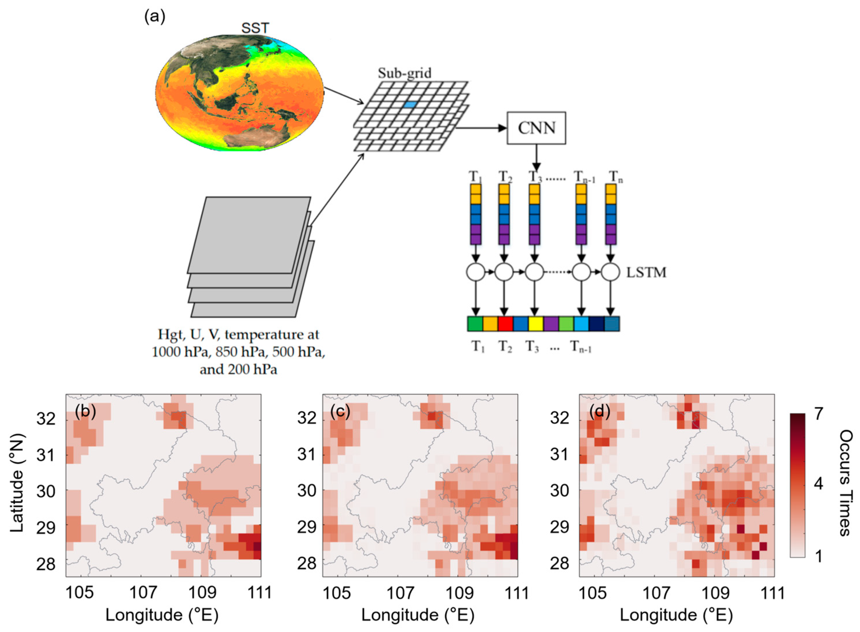
We selected the occur times of extreme precipitation in CSC from June to August in 2000 to 2015 as the training set and the data from 2016 to 2018 in CSC as the test set. For the selection of input features in addition to the conventional variables (Hgt, U, V, temperature at 1000 hPa, 850 hPa, 500 hPa, and 200 hPa), we added an additional SST in the South Indian Ocean (70° W–90° W and 20° S ≤ 0° N) in the control group to investigate whether adding SST as features can improve the forecast results in deep learning. The times of all the input features used in our predict model were in June from 2000 to 2020, which means, for the predicted result of the frequency of extreme precipitation in June, we are exploring a concurrent relationship. But for other months (July and August), it is a lead–lag relationship.
For model training and testing, we chose a relatively reliable algorithm (CNN-LSTM) to undertake the extreme precipitation prediction. Next, we determined the optimal range of the parameters using hyperparameter methods for the training set. The final optimal parameter values were then determined using the K-fold and cross-validation methods for the training set. These optimal parameters were applied to the chosen algorithm (CNN-LSTM). Finally, the testing set was used to verify the accuracy of the extreme precipitation prediction algorithm produced by the training set, and the indicator of the model’s accuracy was calculated (RMSE).
As Figure 6 shows, deep learning is feasible for predicting extreme precipitation, but the results of different algorithms vary somewhat. During the summers of 2016–2018, the observed spatial distribution of extreme precipitation occurrence times (Figure 6b) is similar to the topographic distribution in CSC (Figure 1). The two northern and eastern high-frequency centers (Figure 6b) correspond to the high-value centers of the R95 index (Figure 2). The spatial distribution of the predicted results in the model with SST (Figure 6c) is more consistent with the observed results than that in the the model without SST (Figure 6d). For the model validation, as Table 3 shows, CNN-LSTM generally shows relatively high accuracy in the results of extreme precipitation prediction in CSC. In addition, identifying the key areas of SST which affect CSC precipitation and adding it as an input variable into deep learning algorithms can provide a significant improvement in the results (at least ~50%). This finding provides new ideas for the application of deep learning in extreme precipitation prediction.

4. Discussion

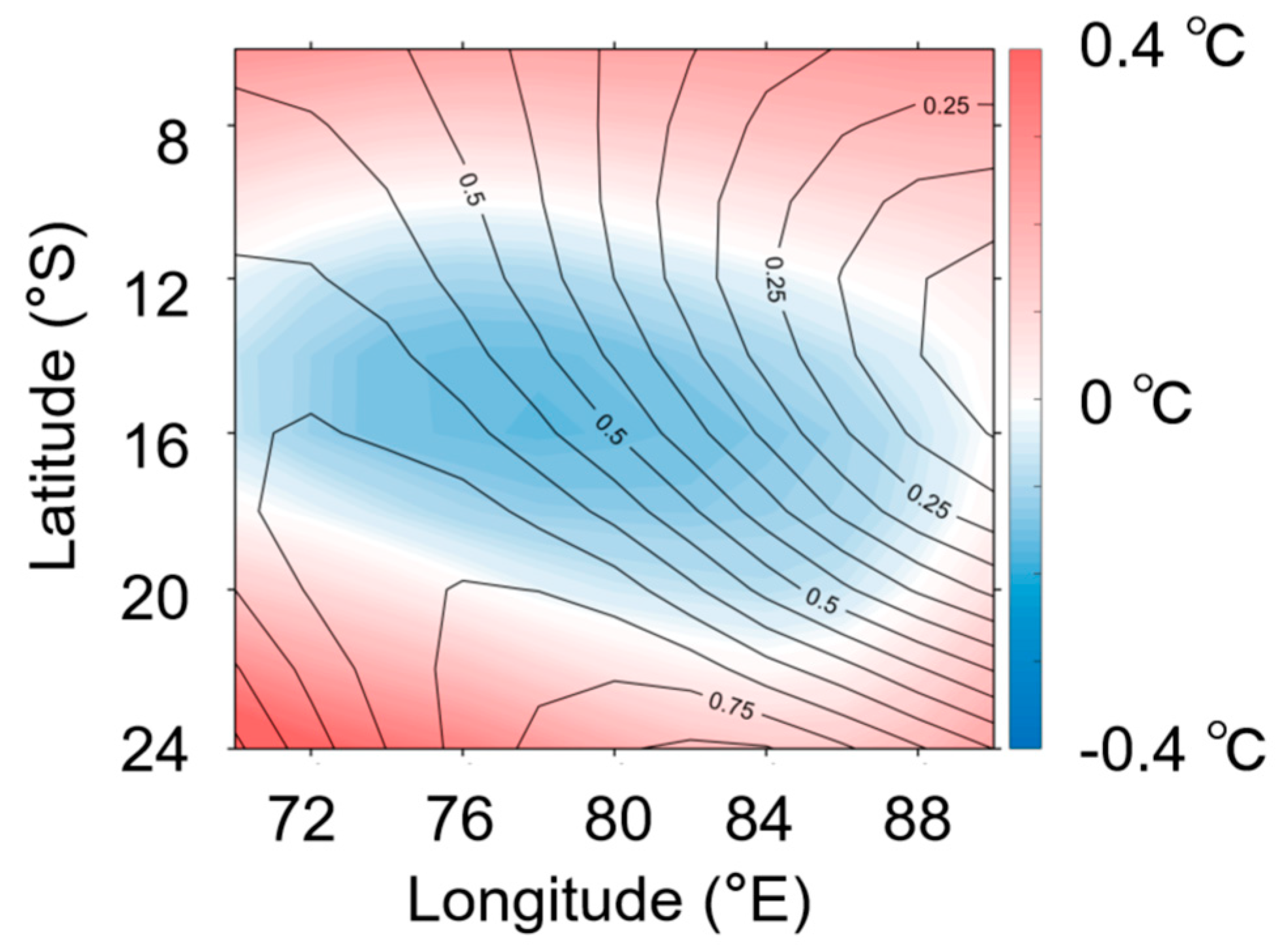
To explore the conjecture mentioned in Section 4, it can be seen that in the time series of the first mode of the EOF (Figure 3b), the occurrence times of extreme precipitation in CSC during the summer of 2011–2013 (this period denoted as Ts) continued to be abnormally lower than those in other years, but during the summer of 2014–2017 (this period denoted as Td), they continued to be abnormally higher than those in other years. Moreover, in Figure 7, the SST anomaly in June of Ts was cold, and the SST anomaly in June of Td was abnormally warm. The abnormal distribution of SST in the South Indian Ocean was in good agreement with the distribution of the first couple of singular vectors in SVD (Figure 5b), which indicated that the two time periods (Ts and Td) were typical. Doswell et al. (1996) [45] provided an ingredient-based framework for thinking about heavy precipitation. These three ingredients involve lift, instability, and moisture. Thus, we analyzed the mechanism of the SST anomaly in the South Indian Ocean affecting the frequency of extreme precipitation in CSC from these components in certain periods (Ts and Td).
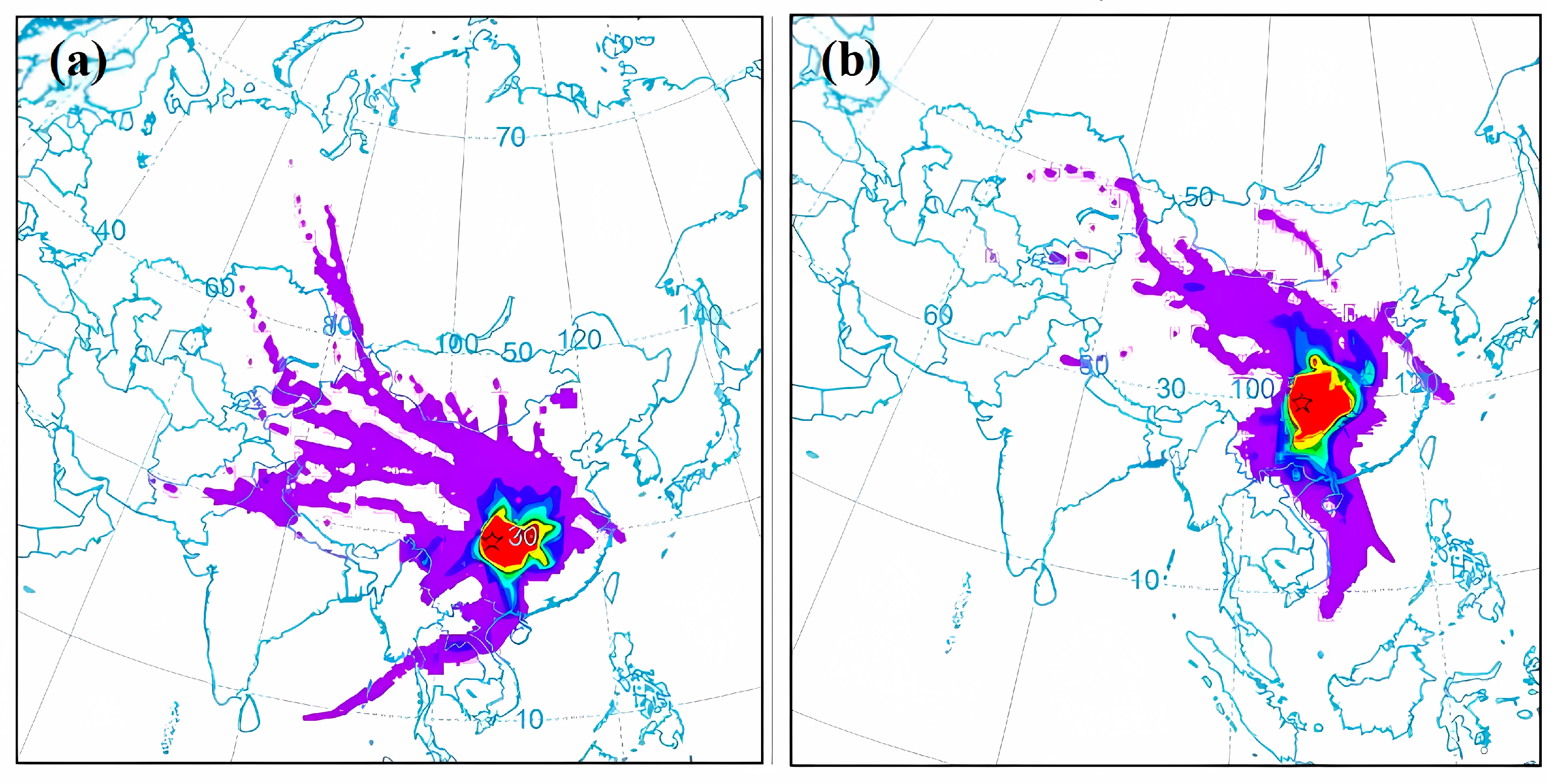
The convergence of cold and warm air causes uplift airflow and unstable stratification. We used the Hysplit trajectory model (Hybrid Single-Particle Lagrangian Integrated Trajectory) to calculate the moving path of the water vapor and cold wave because the source and trajectory path will affect their intensity. The Hysplit model is a widely used atmospheric transport and dispersion model that allows researchers to visualize the movement of air water vapor and other atmospheric constituents over time. Developed by the National Oceanic and Atmospheric Administration (NOAA), it uses a combination of Lagrangian and Eulerian techniques to simulate the trajectories of individual particles or groups of particles, allowing for the prediction of atmospheric concentration patterns. As shown in Figure 8, when the frequency of extreme precipitation decreased (Ts), water vapor was transported from the Indochina Peninsula, and the cold wave in the Ts period invaded CSC through the northwest and west trajectories. When the frequency of extreme precipitation increased (Td), water vapor was transported directly from the South China Sea to CSC, and the cold wave in the Td period invaded CSC through a northwest trajectory. The difference in the cold wave trajectory and the transport path of water vapor lead to the production of different types of extreme precipitation. SST also plays a vital role in determining the transfer of the cold wave trajectory and the transport path of water vapor from the ocean to the atmosphere. One of the primary mechanisms by which SST affects lower atmosphere circulation is through the generation of convective systems over the warmest parts of the ocean. These convective systems can produce large amounts of rainfall, which can affect the temperature and pressure gradients in the atmosphere, leading to changes in wind patterns. Furthermore, the moisture from these convective systems can be transported to other regions, leading to changes in atmospheric moisture levels and precipitation patterns. Therefore, the influence of the SST anomaly on the lower atmosphere circulation would be the key factor in exploring the differences in the frequency of extreme precipitation.
According to the WES (wind–evaporation–SST) positive feedback mechanism [46], a high-pressure system and downward flow exist in the South-Indian Ocean. This downward flow forms meridional circulation with the ascending branch in the Northern Hemisphere, causing cross-equatorial airflow. When the SST in the South Indian Ocean was warm, the temperature difference between the ocean and atmosphere increased, and sensible heating occurred. The converged airflow causes positive vorticity in surface layer t, which weakens the intensity of downward flow and leads to the weakening of the cross-equatorial airflow intensity. Combined in Table 2, the SST anomaly in the Indian Ocean had a strong connection with the cross-equatorial airflow. Therefore, we calculated the anomalous wind speed at 850 hPa in the Ts and Td periods, and the results are shown in Figure 9. Figure 9 shows that when the SST was abnormally cold (Ts), South Asia was under the control of a wide and strong cross-equatorial flow, and the position of the South China Sea summer monsoon was obviously eastward. However, when the SST was warm (Td) and the cross-equatorial airflow intensity was weaker than in other years, the position of the South China Sea monsoon moved eastward, which affected the extreme precipitation in CSC.
In Figure 9, we find a distribution that was the result of complex physical mechanisms. During the Ts period, there was a strong cross-equatorial flow that increased the speed of the westerly wind in the Bay of Bengal region. This led to an eastward expansion of the wind, which, in turn, enhanced the cyclonic circulation over the South China Sea. As a result, the position of the western Pacific subtropical high was controlled over the South China Sea and retreated eastward.
Furthermore, the South China Sea equatorial airflow rapidly intensified during this period, pushing the subtropical high northward. This triggered the full outbreak of the South China Sea summer monsoon. The subtropical high is the sinking branch of the Hadley circulation, and the divergence of air flow takes place at the bottom of its control area. The Hadley circulation is a global-scale atmospheric circulation that features air rising near the equator, flowing poleward near the tropopause, cooling and descending in the subtropics, and then returning equatorward. The subtropical high is the sinking branch of the Hadley circulation, and the divergence of air flow takes place at the bottom of its control area. Therefore, the Hadley circulation can influence the position and intensity of the subtropical high, which, in turn, affects the transport of water vapor and can result in heavy rainfall in the CSC. For example, when the subtropical high was westward, the position of the divergent airflow also moved westward and enhanced the intensity of the South China Sea summer monsoon, which brought water vapor to CSC. When the subtropical high was westward, the position of the divergent airflow also moved westward, enhancing the intensity of the South China Sea summer monsoon. This brought water vapor to the CSC region, resulting in heavier rainfall and flooding.
However, during the Td period, the intensity of the cross-equatorial flow was low, and the South China Sea summer monsoon and the subtropical high showed the opposite response to the cross-equatorial flow.
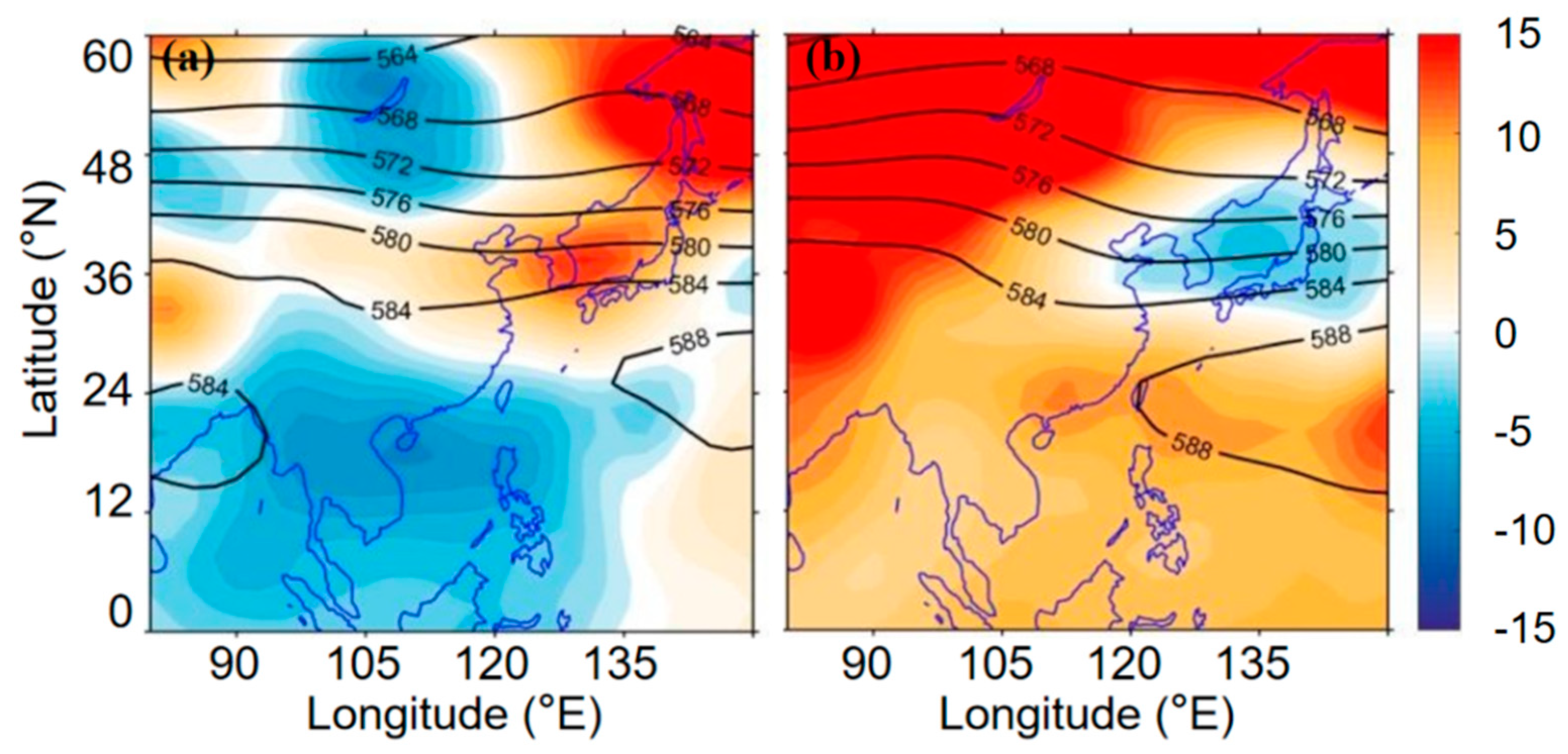
The 500 hPa atmospheric circulation is commonly used in meteorology for weather analysis due to the significant influence of the height field at this level on the interactions between the upper and lower atmosphere. Additionally, the 500 hPa level is typically located at the position of the 500 hPa wind jet, which can reflect the dynamic structure and stability of the atmosphere in the region, thus providing valuable information for weather analysis and forecasting. Furthermore, the 500 hPa height field can also reveal the movement trends of high-altitude weather systems, such as subtropical highs and jet stream waves, which are all factors that affect ground-level weather. As a result, the 500 hPa atmospheric circulation chart has become one of the essential reference tools for weather analysis. By comparing the circulation field at 500 hPa between the two periods (Ts and Td, Figure 10), the difference in the meteorological circulation field at mid–low latitudes between them is mainly reflected in the position and intensity of the subtropical high. In the Ts period, the position of the subtropical high was east, and the intensity was weak. In the Td period, the subtropical high was oriented to the west, and the intensity was strong. This change in intensity and the position of the subtropical high affected the transport of water vapor. The Hadley circulation is a global-scale atmospheric circulation that features air rising near the equator, flowing poleward near the tropopause, cooling and descending in the subtropics, and then returning equatorward. The subtropical high is the sinking branch of the Hadley circulation, and the divergence of air flow takes place at the bottom of its control area. Therefore, the Hadley circulation can influence the position and intensity of the subtropical high, which, in turn, affects the transport of water vapor and can result in heavy rainfall in the CSC. For example, when the subtropical high was westward, the position of the divergent airflow also moved westward and enhanced the intensity of the South China Sea summer monsoon, which brought water vapor to CSC.
In addition, in the middle latitudes (Figure 10), according to the Rossby wave velocity formula, the longer the wavelength is, the easier it is for quasistationary waves to form. In the Ts period, the westerly wave was long and straight at 500 hPa, and this quasistatic wave did not guide the cold air southward to invade CSC. In the Td period, the westerly wave was beneficial to long wave adjustment, and the trough moving eastward also brought cold air and disturbance to precipitation. Therefore, due to cross-equatorial airflow intensity changes, the meteorological circulation and the South China Sea monsoon showed differences in the two periods, causing differences in the trajectory of water vapor. When the water vapor was transported by way of the Indochina Peninsula (Ts period), the mountains and hills in this area hindered this transport. When water vapor is transported from the South China Sea to CSC (Td period), water vapor can reach directly over CSC because the coastal areas of South China are mainly plains. Consequently, the southern mountains in CSC have uplifted water vapor, and the conditions for extreme precipitation have been provided. In addition, the change in intensity of the cross-equatorial flow would affect the convective activity, and then the thermodynamic and dynamic effects of convective activity would affect the meteorological circulation [46,47]. Therefore, the correlation between the convective activity and the vertical movement at 850 hPa over CSC since 1980 was calculated. The results are shown in Table 4. The results showed that the enhancement of convection in the South China Sea is closely related to the descending motions in CSC.
Overall, according to Figure 9 and Figure 10, the physical mechanisms that led to the difference distributions in extreme precipitation were multifaceted, involving the cross-equatorial flow, the position and intensity of the subtropical high, and the South China Sea equatorial airflow. These factors have significant impacts on weather patterns in the region and can result in different extreme precipitation events.
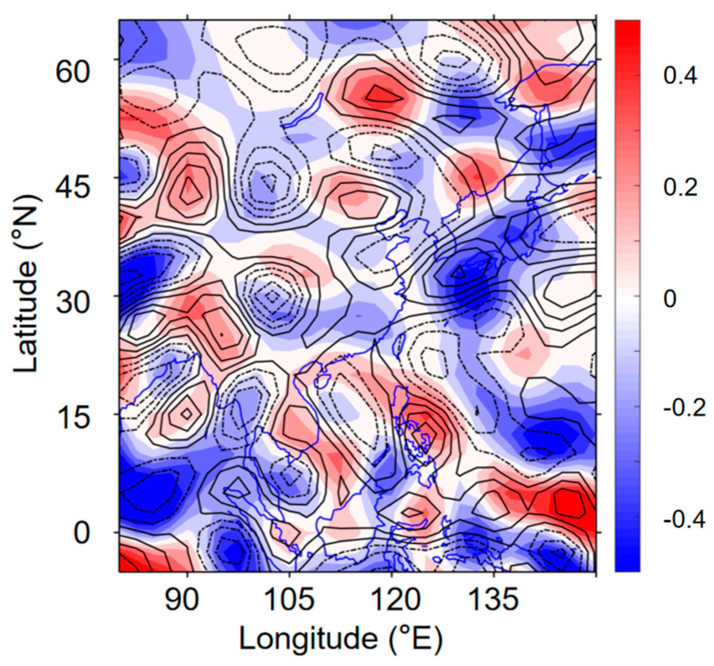
We calculated the vorticity anomaly, and the results are shown in Figure 11. During the Ts period, the vorticity anomaly in CSC was negative, while the anomaly was positive during the Td period. Moreover, in Figure 11, all of the Ts and Td periods showed significant Pacific–Japan (PJ) teleconnection wave trains. However, there was a large difference in the location and travel path between the PJ teleconnection wave trains in the two periods. Nitta [42] found that the PJ teleconnection wave train was excited by convection over the Philippine Sea in summer. This is probably due to the change in the convective activity center caused by the change in the cross-equatorial airflow intensity, which affects the position and path of the PJ wave train. In Figure 11, the enhanced cross-equatorial airflow caused convective activity, and major teleconnection centers occurred in the South China Sea. The PJ teleconnection wave train experienced a marked variation with its major teleconnection centers shifting southwestward. The negative PJ phases led to downdraft in CSC, which is not conducive to extreme precipitation. In the Td period, convective activity occurred in the Philippines, causing the PJ teleconnection wave train to propagate from the Philippines to the Sea of Japan. The positive PJ phases caused the uplift airflow in CSC, which is beneficial to extreme precipitation. Therefore, the SST anomaly in the South Indian Ocean can affect the water vapor trajectory and uplift movement of CSC by changing the intensity of cross-equatorial airflow, thus affecting the extreme precipitation in CSC.

5. Conclusions

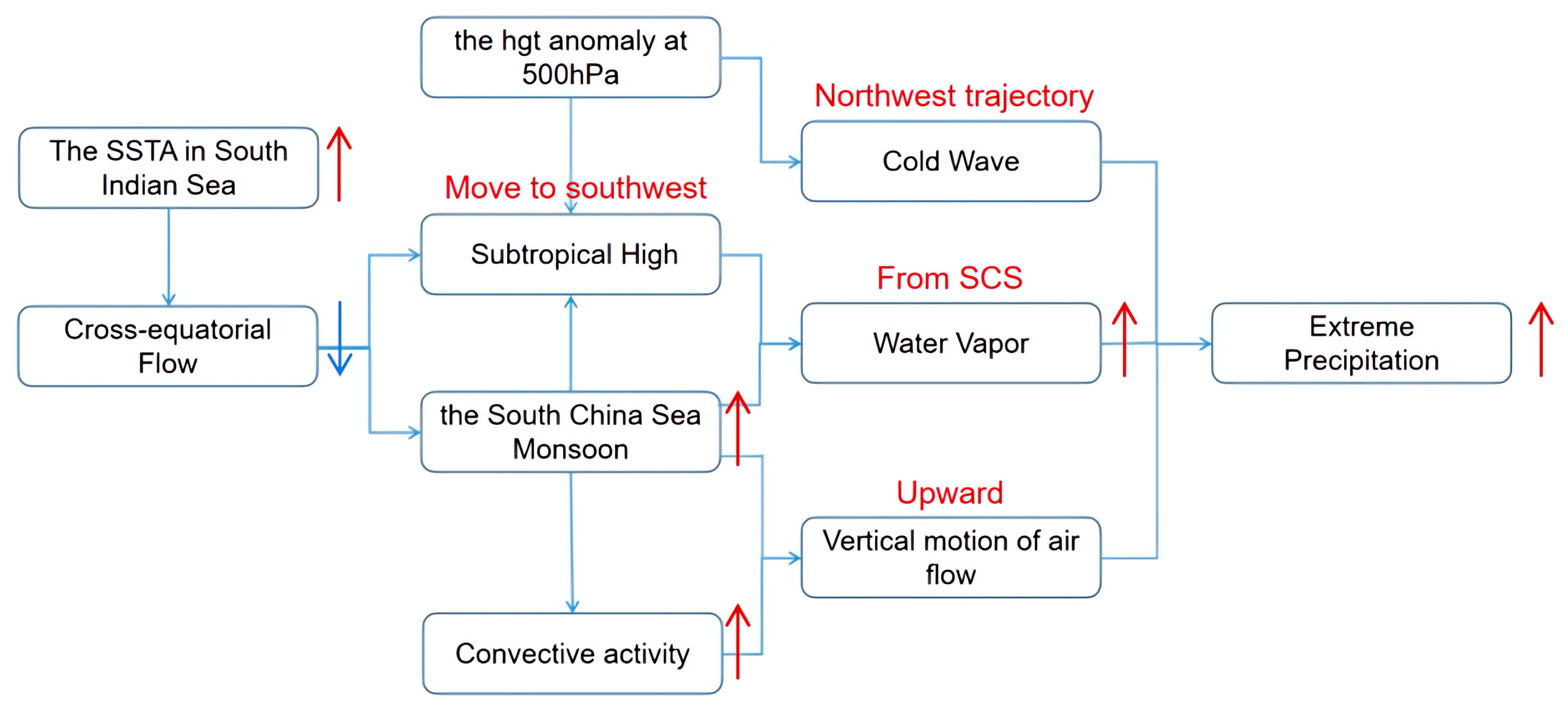
In this paper, we used a variety of statistical methods to analyze the distribution of extreme precipitation in CSC. The results showed that the temporal distribution of extreme precipitation in CSC had a consistent pattern, but due to the terrain, it also showed the opposite phase between the north and the south in spatial distribution, and the fluctuation was obvious in the time series. The mechanism of the impact of SST anomalies on extreme precipitation can be seen in Figure 12.
When the temperature of the sea surface in the South Indian Ocean changes, it can trigger abnormal sensible heating in the atmosphere. This, in turn, leads to a change in the distribution of heat and moisture around the planet. Specifically, the converged airflow caused by this heating can result in shifts in the gradient of hgt (geopotential height field) between the northern and southern hemispheres.
These shifts in the gradient of hgt can have significant impacts on weather patterns around the world, as they can alter the intensity of cross-equatorial air flow. This alteration affects the position of the subtropical high and the intensity of the South China Sea summer monsoon.
The summer monsoon is responsible for heavy rainfall and flooding in Southeast Asia each year, and its intensity and location can vary from year to year. When the intensity of the summer monsoon changes, it can alter the trajectory of water vapor transport and create different paths for water vapor to follow. The location of the subtropical high also influences the trajectory of water vapor transport, so when both the summer monsoon and subtropical high shift in intensity or position, it can lead to significant changes in precipitation patterns.
In addition to altering precipitation patterns, variations in the intensity of the South China Sea summer monsoon can also impact the convective activity of the region. Convective activity refers to the vertical movement of air flow over the South China Sea, which is influenced by the PJ teleconnection wave train. This large-scale atmospheric wave pattern spans across the Pacific Ocean, connecting regions in the western North Pacific with those in the eastern tropical Pacific.
As a result of these factors, extreme precipitation events in the CSC region can be triggered by a complex interplay of trajectories of cold air and water vapor, the vertical movement of air flow, and convective activity. The frequency of these events can be influenced by changes in the SST of the South Indian Ocean, the intensity of the summer monsoon and subtropical high, and the influence of the PJ teleconnection wave train.
In conclusion, as Figure 12 shows, when the SST of the South Indian Ocean changes, because of abnormal sensible heating, the converged airflow changes the gradient of the hgt between the northern and southern hemispheres, which will lead to a change in the intensity of the cross-equatorial air flow. This change affects the intensity of the South China Sea summer monsoon and the position of the subtropical high. Under the interaction of the summer monsoon and subtropical high, the trajectory of water vapor transport appears to have different paths. At the same time, the variation in summer monsoon intensity also affects the convective activity of the South China Sea and then influences the vertical motion of air flow over CSC by the PJ teleconnection wave train. Thus, the combination of the trajectory of cold air and water vapor and the vertical movement together affect the frequency of extreme precipitation in CSC. However, the time period of the available dataset should be extended, and future collaborations with local authorities should be considered to obtain precipitation data over a longer time span. This will facilitate iterative updates of the model.

Author Contributions

S.L., Y.L. and Z.W. participated in the in situ data collection. S.L., S.Y. and Z.W. developed the prediction method, wrote the codes, analyzed the data, and plotted the figures. S.L. and S.Y. wrote the paper. J.S. and Z.W. contributed to the writing, editing, and revising of the draft of this paper. All authors have read and agreed to the published version of the manuscript.

Funding

This research was funded by State Key Program of National Natural Science of China (Grant No. 41430963).

Data Availability Statement

Data are contained within the article.

Conflicts of Interest

The authors declare no conflicts of interest.

References

  1. IPCC. Climate Change 2022: Impacts, Adaptation, and Vulnerability. Contribution of Working Group II to the Sixth Assessment Report of the Intergovernmental Panel on Climate Change; Cambridge University Press: Cambridge, UK; New York, NY, USA, 2022; 3056p.
  2. Easterling, D.R.; Evans, J.L.; Groisman, P.Y.; Karl, T.R.; Kunkel, K.E.; Ambenje, P. Observed variability and trends in extreme climate events: A brief review. Bull. Am. Meteorol. Soc. 2000, 81, 417–425. [Google Scholar] [CrossRef]
  3. Kendon, E.J.; Roberts, N.M.; Fowler, H.J.; Roberts, M.J.; Chan, S.C.; Senior, C.A. Heavier summer downpours with climate change revealed by weather forecast resolution model. Nat. Clim. 2014, 4, 570–576. [Google Scholar] [CrossRef]
  4. Capello, M. Changes in the physical characteristics of the water column at the mouth of a torrent during an extreme rainfall event. J. Hydrol. 2016, 541, 146–157. [Google Scholar] [CrossRef]
  5. Zhang, X.; Zwiers, F.W.; Li, G.; Wan, H.; Cannon, A.J. Complexity in estimating past and future extreme short-duration rainfall. Nat. Geosci. 2017, 10, 255–259. [Google Scholar] [CrossRef]
  6. Cramer, S.; Kampouridis, M.; Freitas, A.A.; Alexandridis, A.K. An extensive evaluation of seven machine learning methods for rainfall prediction in weather derivatives. Expert Syst. Appl. 2017, 85, 169–181. [Google Scholar] [CrossRef]
  7. Di, Y.; Ding, W.; Mu, Y.; Small, D.L.; Islam, S.; Chang, N.-B. Developing machine learning tools for long-lead heavy precipitation prediction with multi-sensor data. In Proceedings of the 2015 IEEE 12th International Conference on Networking, Sensing and Control, Taipei, Taiwan, 9–11 April 2015. [Google Scholar]
  8. Knighton, J.; Pleiss, G.; Carter, E.; Lyon, S.; Walter, M.T.; Steinschneider, S. Potential predictability of regional precipitation and discharge extremes using synoptic-scale climate information via machine learning: An evaluation for the eastern continental United States. J. Hydrometeorol. 2019, 20, 883–900. [Google Scholar] [CrossRef]
  9. Molina, M.J.; Gagne, D.J.; Prein, A.F. A benchmark to test generalization capabilities of deep learning methods to classify severe convective storms in a changing climate. Earth Space Sci. 2021, 8, e2020EA001490. [Google Scholar] [CrossRef]
  10. Charlesworth, E.; Plöger, F.; Birner, T.; Baikhadzhaev, R.; Abalos, M.; Abraham, N.L.; Akiyoshi, H.; Bekki, S.; Dennison, F.; Jöckel, P.; et al. Stratospheric water vapor affecting atmospheric circulation. Nat. Commun. 2023, 14, 3925. [Google Scholar] [CrossRef]
  11. Tang, Y.; Huangfu, J.; Huang, R.; Chen, W. Surface warming reacceleration in offshore China and its interdecadal effects on the East Asia–Pacific climate. Sci. Rep. 2020, 10, 14811. [Google Scholar] [CrossRef]
  12. Wu, X.; Guo, S.; Yin, J.; Yang, G.; Zhong, Y.; Liu, D. On the event-based extreme precipitation across china: Time distribution patterns, trends, and return levels. J. Hydrol. 2018, 562, 305–317. [Google Scholar] [CrossRef]
  13. Lu, C.; Lott, F.C.; Sun, Y.; Stott, P.A.; Christidis, N. Detectable anthropogenic influence on changes in summer precipitation in China. J. Clim. 2022, 33, 5357–5369. [Google Scholar] [CrossRef]
  14. Sun, J.; Zhang, F.Q. Daily extreme precipitation and trends over China. Sci. China Earth Sci. 2017, 44, 1689–1701. [Google Scholar] [CrossRef]
  15. Guo, J.; Huang, G.; Wang, X.; Li, Y.; Yang, L. Future changes in precipitation extremes over China projected by a regional climate model ensemble. Atmos. Environ. 2018, 188, 142–156. [Google Scholar] [CrossRef]
  16. Xiao, C.; Wu, P.; Zhang, L.; Song, L. Robust increase in extreme summer rainfall intensity during the past four decades observed in China. Sci. Rep. 2016, 6, 38506. [Google Scholar] [CrossRef] [PubMed]
  17. Zhai, P.; Zhang, X.; Wan, H. Trends in total precipitation and frequency of daily precipitation extremes over China. J. Clim. 2005, 18, 1096–1108. [Google Scholar] [CrossRef]
  18. Lau, N.C.; Nath, M.J. A Model Investigation of the Role of Air–Sea Interaction in the Climatological Evolution and ENSO-Related Variability of the Summer Monsoon over the South China Sea and Western North Pacific. J. Clim. 2009, 22, 4771–4792. [Google Scholar] [CrossRef]
  19. Gu, X.; Ye, L.; Xin, Q.; Zhang, C.; Zeng, F.; Nerantzaki, S.D.; Papalexiou, S.M. Extreme Precipitation in China: A Review on Statistical Methods and Applications. Adv. Water Resour. 2022, 163, 104144. [Google Scholar] [CrossRef]
  20. Yu, S.; Luo, Y.; Wu, C.; Zheng, D.; Liu, X.; Xu, W. Convective and microphysical characteristics of extreme precipitation revealed by multisource observations over the pearl river delta at monsoon coast. Geophys. Res. Lett. 2022, 49, e2021GL097043. [Google Scholar] [CrossRef]
  21. Ding, T.; Ke, Z. A Comparison of statistical approaches for seasonal precipitation prediction in Pakistan. Weather Forecast. 2013, 28, 1116–1132. [Google Scholar] [CrossRef]
  22. Li, J.; Wang, B. Predictability of summer extreme precipitation days over eastern China. Clim. Dyn. 2018, 51, 4543–4554. [Google Scholar] [CrossRef]
  23. Han, T.; Wang, H.; Hao, X.; Li, S. Seasonal Prediction of Midsummer Extreme Precipitation Days over Northeast China. J. Appl. Meteorol. Climatol. 2019, 58, 2033–2048. [Google Scholar] [CrossRef]
  24. Szturc, J.; Ośródka, K.; Jurczyk, A.; Otop, I.; Linkowska, J.; Bochenek, B.; Pasierb, M. Quality control and verification of precipitation observations, estimates, and forecasts. In Precipitation Science; Michaelides, S., Ed.; Elsevier: Amsterdam, The Netherlands, 2022; Volume 3, pp. 91–133. [Google Scholar]
  25. Kalnay, E.; Kanamitsu, M.; Kistler, R.; Collins, W.; Deaven, D.; Gandin, L.; Iredell, M.; Saha, S.; White, G.; Woollen, J.; et al. The NCEP/NCAR 40-Year reanalysis project. Bull. Am. Meteorol. Soc. 1996, 77, 437–471. [Google Scholar] [CrossRef]
  26. Reynolds, R.W.; Smith, T.M.; Liu, C.; Chelton, D.B.; Casey, K.S.; Schlax, M.G. Daily high-resolution blended analyses for sea surface temperature. J. Clim. 2007, 20, 5473–5496. [Google Scholar] [CrossRef]
  27. Frich, P.; Alexander, L.; Dellamarta, P.; Gleason, B.; Haylock, M.; Tank, A.; Peterson, T. Observed coherent changes in climatic extremes during the second half of the twentieth centur. Clim. Res. 2002, 19, 193–212. [Google Scholar] [CrossRef]
  28. Farge, M. Wavelet transforms and their applications to turbulence. Annu. Rev. Fluid Mech. 1992, 24, 395–457. [Google Scholar] [CrossRef]
  29. Pearson, K. On lines and planes of closest fit to system of points in space. Philos. Mag. 1902, 2, 559–572. [Google Scholar] [CrossRef]
  30. Cui, D.X.; Liu, W.Y. Application of empirical orthogonal function resolution to analysis of crustal vertical deformation field. Earthquake 2000, 20, 82–86. [Google Scholar]
  31. Bretherton, C.S.; Smith, C.; Wallace, J.M. An intercomparison of methods for finding coupled patterns in climate data. J. Clim. 1992, 5, 541–560. [Google Scholar] [CrossRef]
  32. Wallance, J.M.; Smith, C.; Bretherton, C.S. Singular value decomposition of wintertime sea surface temperature and 500 mb height anomalies. J. Clim. 1992, 5, 561–576. [Google Scholar] [CrossRef]
  33. Lawrence, S.; Giles, C.L.; Tsoi, A.C.; Back, A.D.; Report, T. Face Recognition: A Hybrid Neural Network Approach. In IEEE International Multi Topic Conference; IEEE: New York, NY, USA, 1997. [Google Scholar]
  34. Krizhevsky, A.; Sutskever, I.; Hinton, G. Imagenet classification with deep convolutional neural networks. Adv. Neural Inf. Process. Syst. 2012, 25. [Google Scholar] [CrossRef]
  35. Nagi, J.; Ducatelle, F.; Caro GA, D.; Ciresan, D.; Gambardella, L.M. Max-pooling convolutional neural networks for vision-based hand gesture recognition. In Proceedings of the IEEE International Conference on Signal & Image Processing Applications, Kuala Lumpur, Malaysia, 16–18 November 2011; IEEE: New York, NY, USA. [Google Scholar]
  36. Wu, S.; Lew, M. Comparison of Information Loss Architectures in CNNs. In Proceedings of the 17th Pacific-Rim Conference on Multimedia, Xi’an, China, 15–16 September 2016; Springer: Cham, Switzerland, 2016. [Google Scholar]
  37. Salehinejad, H.; Sankar, S.; Barfett, J.; Colak, E.; Valaee, S. Recent Adv. Recurr. Neural Networks. arXiv 2017, arXiv:1801.01078. [Google Scholar]
  38. Hochreiter, S.; Schmidhuber, J. Long short-term memory. Neural Comput. 1997, 9, 1735–1780. [Google Scholar] [CrossRef]
  39. Graves, A. Sequence transduction with recurrent neural networks. Comput. Sci. 2012, 58, 235–242. [Google Scholar]
  40. Agga, A.; Abbou, A.; Labbadi, M.; El Houm, Y.; Ali, I.H.O. CNN-LSTM: An efficient hybrid deep learning architecture for predicting short-term photovoltaic power production. Electr. Power Syst. Res. 2022, 208, 107908. [Google Scholar] [CrossRef]
  41. Hodson, T. Root mean square error (RMSE) or mean absolute error (MAE): When to use them or not. Electr. Power Syst. Res. 2022, 15, 5481–5487. [Google Scholar] [CrossRef]
  42. Nitta, T. Unusual summer weather over Japan in 1988 and its relationship to the Tropics. J. Meteorol. Soc. Jpn. 1990, 68, 575–587. [Google Scholar] [CrossRef]
  43. Yuan, Y.; Yang, S. Impacts of different types of El Niño on the East Asian climate: Focus on ENSO cycles. J. Clim. 2012, 25, 7702–7722. [Google Scholar] [CrossRef]
  44. Zhang, Y.; Zhou, W.; Wang, X.; Chen, S.; Chen, J.; Li, S. Indian Ocean Dipole and ENSO’s mechanistic importance in modulating the ensuing-summer precipitation over Eastern China. npj Clim. Atmos. Sci. 2022, 5, 48. [Google Scholar] [CrossRef]
  45. Doswell, C.A., III; Brooks, H.E.; Maddox, R.A. Flash flood forecasting: An ingredients-based methodology. Weather Forecast. 1996, 11, 560–581. [Google Scholar]
  46. Wang, B.; Gao, Z.; Chen, F.; Lu, C. Impact of Tibetan Plateau surfaceheating on persistent extreme precipitation events in southeastern China. Mon. Weather Rev. 2017, 145, 3485–3505. [Google Scholar]
  47. Xie, S.P.; Yan, D.; Gang, H. Decadal shift in El Niño influences on Indo -Western Pacificand East Asian climate in the 1970s. J. Clim. 2010, 23, 3352–3368. [Google Scholar] [CrossRef]
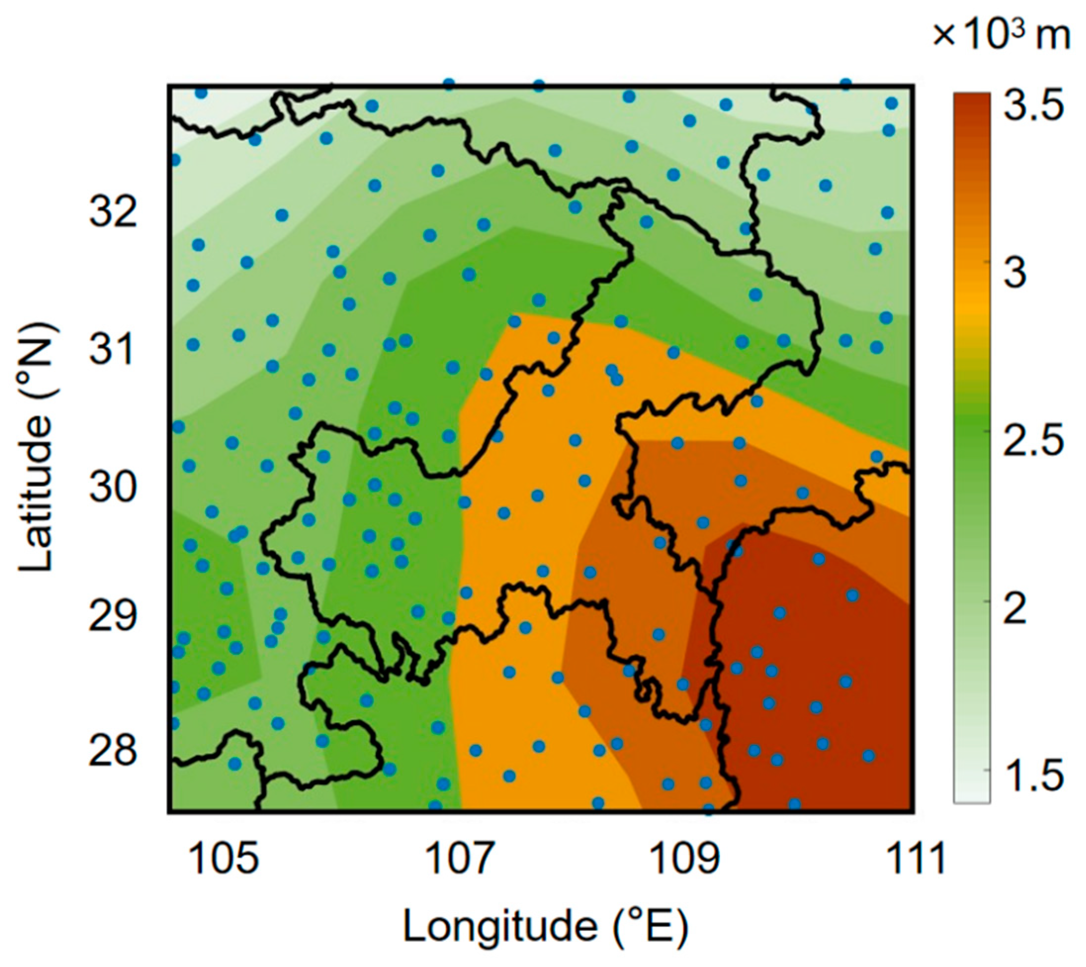
Figure 1. The distribution of atmospheric automatic monitoring stations (pointed) and topography of CSC (shaded part, units: 102 m).
Water 16 00427 g001
Figure 2. The distribution of the daily summer extreme precipitation index (R95) in the CSC.
Water 16 00427 g002
Figure 3. The EOF modes of the summer extreme precipitation frequency in the CSC. (a) Eigenvector distribution and (b) principal component time series of the first EOF mode; (c) eigenvector distribution and (d) principal component time series of the second EOF mode.
Water 16 00427 g003
Figure 4. Wavelet power spectrum of the frequency of extreme precipitation in summer over CSC (the blue circles in the wavelet spectrum represent the 95% confidence interval).
Water 16 00427 g004
Figure 5. Spatial distributions of the first couple singular vectors of (a) the frequency of summer extreme precipitation and (b) SST anomaly in June from SVD analysis (the black line stands for the 95% confidence interval).
Water 16 00427 g005
Figure 6. Framework of spatiotemporal deep neural network fusion model (a). and the spatial distribution of averaged occurrence times of summer extreme precipitation in CSC during 2016 to 2018 ((b). Observational results; (c). Model results with SST; (d). Model results without SST). The spatiotemporal deep neural network fusion model consists of two parts: a CNN spatial feature extraction module and an LSTM module. The CNN spatial feature extraction module mainly extracts feature vectors related to precipitation at the grid center point. The LSTM module is used to capture the temporal correlation of precipitation.
Water 16 00427 g006
Figure 7. The distribution of SST anomalies in the Ts period (shaded part, units: °C) or Td period (lines part, units: °C).
Water 16 00427 g007
Figure 8. The Hysplit model result at 850 hPa in (a). Ts period and (b). Td period over CSC (100 * number of endpoints per grid square/number of trajectories, shaded).
Water 16 00427 g008
Figure 9. The distribution of anomalous wind (the arrow-line) and the anomalous value of u-wind (shaded) at 850 hPa in (a). Ts and (b). Td (units: m/s).
Water 16 00427 g009
Figure 10. The height anomaly (1 gpm, shading) and average height (contour interval = 10 gpm) at 500 hPa in (a). Ts period and (b). Td period.
Water 16 00427 g010
Figure 11. The distribution of the vorticity anomaly in the Ts period (contour interval = 10−6/s) and Td period (shaded, units = 10−5/s) and the PJ teleconnection wave train in the Ts period (yellow line) and Td period (gray line).
Water 16 00427 g011
Figure 12. The mechanism of the impact of SST anomalies on extreme precipitation in CSC.
Water 16 00427 g012
Table 1. Variance contribution rate of each mode of the EOF.
First ModeSecond ModeThird Mode
Variance Contribution40.12%21.83%8.49%
Accumulated-61.95%70.44%
Table 2. The SIG value of the correlation coefficient between the north–south potential latitude gradient and the v-wind speed at low latitudes.
JuneJulyAugust
Correlation Coefficient0.53620.48870.4170
SIG value0.00010.00030.0026
Table 3. The RMSE and R2, associated with different algorithms for different features in the test set of summer.
FeaturesJune
(RMSE/R2)
July
(RMSE/R2)
August
(RMSE/R2)
Summer
(RMSE/R2)
No SST0.32/0.750.33/0.710.39/0.710.35/0.73
SST0.11/0.850.06/0.890.07/0.860.09/0.85
Table 4. Correlation coefficient between OLR and vertical movement in CSC (the yellow part stands for the 95% confidence interval).
Philippine SeaSouth China SeaBay of Bengal
Vertical Movement0.060.410.10
Disclaimer/Publisher’s Note: The statements, opinions and data contained in all publications are solely those of the individual author(s) and contributor(s) and not of MDPI and/or the editor(s). MDPI and/or the editor(s) disclaim responsibility for any injury to people or property resulting from any ideas, methods, instructions or products referred to in the content.