Failure Prediction of Open-Pit Mine Landslides Containing Complex Geological Structures Using the Inverse Velocity Method

Abstract

In the field of open-pit geological risk management, landslide failure time prediction is one of the important topics. Based on the analysis of displacement monitoring data, the inverse velocity method (INV) has become an effective method to solve this issue. To improve the reliability of landslide prediction, four filters were used to test the velocity time series, and the effect of landslide failure time prediction was compared and analyzed. The results show that the sliding process of landslide can be divided into three stages based on the INV: the initial attenuation stage (regressive stage), the second attenuation stage (progressive stage), and the linear reduction stage (autoregressive stage). The accuracy of the INV is closely related to the measured noise of the monitoring equipment and the natural noise of the environment, which will affect the identification of different deformation stages. Compared with the raw data and the exponential smoothing filter (ESF) models, the fitting effect of the short-term smoothing filter (SSF) and long-term smoothing filter (LSF) in the linear autoregressive stage is better. A stratified prediction method combining SSF and LSF is proposed. The prediction method is divided into two levels, and the application of this method is given.

1. Introduction

Rockfalls and ground surface deformation, which are notoriously known due to their strong abruptness, intermittent occurrence, and destructive harm, are among the most critical issues both during mining and for many years after the cessation of mining [1,2]. In open-pit mining (also known as open-cut or open-cast mining), geomorphic processes possibly result in slope failures with alterations that entail potential sources of risk to personnel, apparatus, and infrastructures, in addition to dislocating mining scenarios and multiplying production expenditures [3,4,5]. Nevertheless, production work at a high rate could be hindered by major slope failure or the over-conservative nature of the ultimate design [6,7,8]. The mitigation of slope failure is a crucial topic of particular concern in open-pit mines, where production works must proceed with economic benefit yield, and simultaneously the safety of the personnel and the integrity of the mining equipment must be guaranteed [9].

Discerning ongoing processes of rock slope deformation that may lead to instability covers essential miscellaneous aspects of engineering geology and geomechanics [10,11,12]. The management of and substantial information on slope failure-associated risks are integral to having an adequate understanding of the lithostructural predisposition, the driving forces, and the different mechanisms and environmental conditions in the monitored area [13,14,15]. Irrespective of spatial and temporal terms, displacement and its derivatives (velocity and acceleration) are widely considered to be the most reliable alert indicators that can provide an early warning of potential movements [16]. Systematic efforts have gone into implementation for early-warning precautions of a near-real-time slope monitoring network by utilizing the correlation among these kinematic parameters. The rationale for the majority failure forecast method (FFM) [17] is based on the observation that slopes undergo velocity increases asymptotically towards failure (“tertiary” or “accelerating” creep) [18]. Albeit clearly, FFM is on the temporal prediction of landslides and imminent collapse, which can be defined as time-of-failure (TOF) [19]. This leads to the necessity of integrating TOF analysis and alert indicators with a real-time assessment tool. Such a precursory tool was first suggested by Saito [20], incorporating discovering the inversely proportional relationship between time to slope failure and existing strain rate within the tertiary creep phase, and later improved by Fukuzono [21], who introduced a phenomenological method that takes into account the inverse of the velocity against time, the so-call inverse velocity (INV) method, leading to effective forecast results before the ultimate failure. Voight [22,23] went on to present successful applications of this method and extended the results to other types of natural phenomena or failure mechanisms, e.g., volcanic eruptions. Astonishingly, although the INV method was developed based on laboratory tests more than 30 years ago, it does not appear to have achieved implementation and verification for real-time slope failure prediction in the mining industry or mining-related technical literature until 2001 [24]. Since the early 21st century, in order to develop approaches to evaluate the failure time (t_f) of landslides, published examples (from the investigation of some large open-pit slope failures) of successful implementation are proposed to predict impending failure based on the results of the conventional application of INV methods [25,26,27,28].

Several studies of the INV method have been carried out to define rules and procedures to estimate the time of landslides in open-pit mines, including Rose and Hungr [24], Mufundirwa et al. [29], Dick et al. [19], Carlà et al. [30,31], Zhou et al. [32], and Chen and Jiang [33]. By presenting three large rockfall events of open-pit mines (1, 2, and 18 million m³) in Northeastern Nevada, Rose and Hungr [24] demonstrated the accuracy and efficacy of this method. The result of the largest event was even forecasted 3 months before the impending failure. Dick et al. [19] further discussed the application of the INV method in open-pit mines by using new systematic multi-pixel and machine-learning models to complement the scarcity of conventional geodetic monitoring programs for near-real-time deformation measurements. Carlà et al. [9] took an anonymous copper open-pit mine into account and defined the appropriate strategy for the setup of alarms, which were deduced from the presented nine cases of slope instability and the relationship between the reciprocal displacement rate and duration time in the accelerating stage before the slope failure. To address the reliability of the prediction method and simultaneously provide guidelines for the proficient usage of this method, Zhou et al. [32] developed the modified INV method when analyzing the five landslides of Fushun West Pit slope failure. Similarly, Chen and Jiang [33] supposed that the selection of thresholds is usually over-conservative, considering the low-risk tolerance, and therefore introduced a dimensionless inverse velocity method (DINV) to provide a general solution framework that was used to assess the slope failure risk and avoid false alarms. The main characteristic of the inverse velocity method is its simplicity of use which has provided a useful tool for the interpretation of instrument data to anticipate eventual slope failure. These developments notwithstanding, the practical usefulness of the INV method for early warning in open-pit mines may be fairly constrained because of the following major drawbacks. In general, the INV method was formulated from fixed and human-controlled laboratory conditions, which are extremely unlikely to suffice in engineering slopes and field conditions. Furthermore, limitations connected to previous point-wise monitoring analysis of the INV method in open-pit mines are significant, often resulting in undersampled or poorly collected data. Additionally, the surface mining environment produces manifold noise patterns (e.g., mining extraction action, transportation equipment destabilization, human activities, measurement errors, etc.), which are considered to be a defect for early-warning purposes. Finally, the prediction performance of the INV method under different displacement scales does not appear to have been analyzed to date. All these mentioned gaps can decisively hinder the interpretation of the inverse velocity plot and affect the precision and dependability of t_f prediction.

In this context, it is essential to propose the application of a conventional inverse modeling tool, based on the moving average transfer function, for eliminating as many as possible disturbing effects related to the prediction of displacements and compensating for other defects. To manifest the feasibility and punctuality of the FINV (filter inverse velocity) method for time-of-failure analyses in a mining environment, the back analysis of a large slope failure that occurred in August 2016 at Fushun, an open-pit coal mine in northeast China, is examined in detail. On this basis, we examined velocity time series using four filters and analyzed the validity of landslide damage time predictions.

2. Materials and Methods

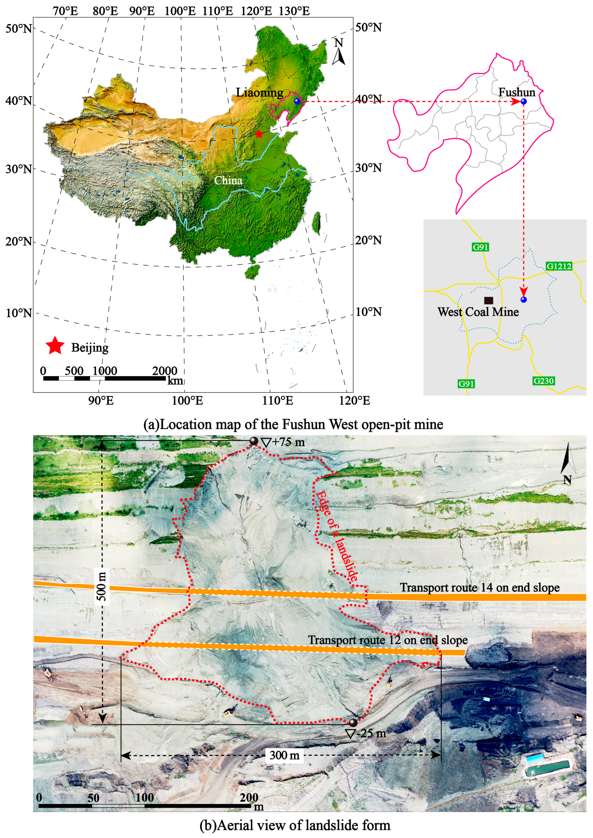
2.1. Study Area

The Fushun West open-pit mine is located in the western part of the Fushun coalfield, at the northern foot of Qiantai Mountain on the southern bank of the Hun River. The geographical coordinates of the mine range from approximately 41°38′0″ N to 42°14′0″ N and 123°39′12″ E to 124°28′0″ E, as shown in Figure 1a. The open pit has a length of approximately 6.6 km, a width of around 2.2 km, and a total area of about 14.52 km². The mining depth reaches 400 m. However, the Fushun West open-pit mine faces serious landslide hazards due to factors including open-pit mining, underground excavation, faults, and weak layers. Specifically, the mine has experienced over 900 collapse events attributable to landslides. More than 50% of these incidents occurred from June to September when rainfall is relatively concentrated. These landslide events have resulted in a total damaged area of 635,000 m² and have given rise to a series of safety and geological environmental issues concerning open-pit mining.

On the evening of 25 July 2016, the Fushun area was struck by a rainfall event with a return period of 50 years, resulting in nearly 200 mm of precipitation. At 5:00 a.m. the following day, a partial landslide occurred on the northern slope of the Fushun West open-pit mine, as shown in Figure 1b. The elevation of the landslide’s rear edge was approximately +75 m, while the shear location at the front edge was around −25 m. The landslide spanned a north–south width of approximately 300 m, with a height difference of 110 m, and with an east–west width of approximately 500 m. The total area affected by the landslide was approximately 150,000 m². The landslide caused the burial of the bottom sections 12 and 14 of the mainline, with the sliding tongue extending. This resulted in the complete interruption of the internal electrical railway lines in the eastern section of the mine, as well as the disruption of the western slope’s transportation roads, including the Xingping Road and the car transport highway. These disruptions had a significant impact on the internal drainage of the eastern open pit and the upper soil removal in the western area of the mine, severely impeding normal production in the mining area.

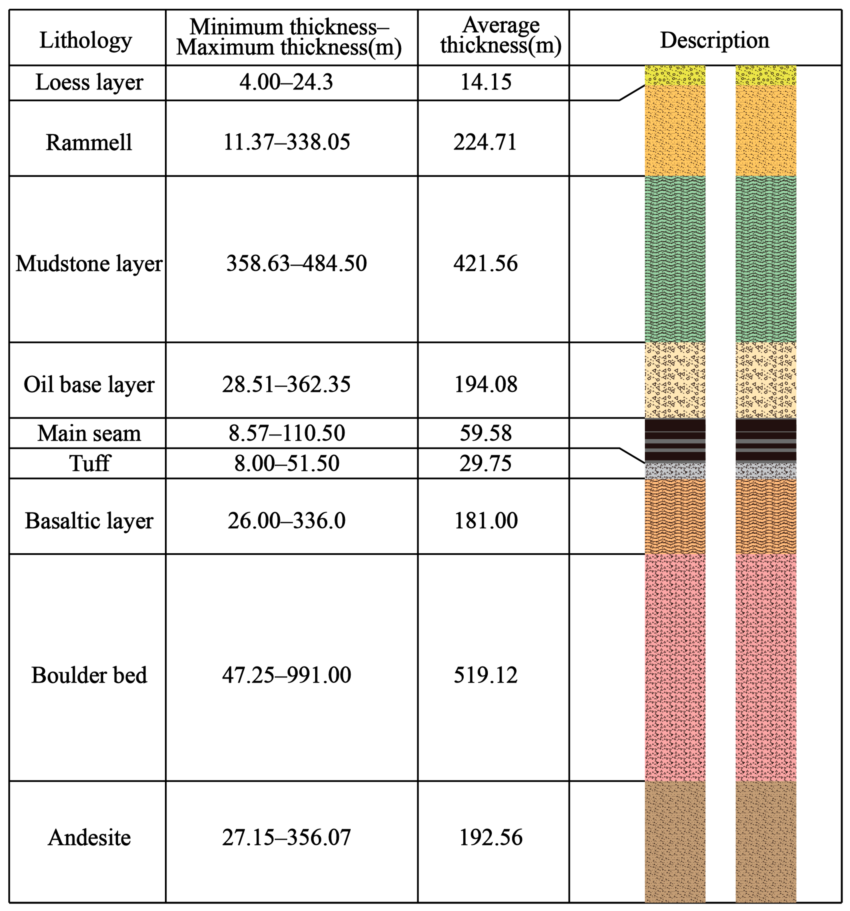
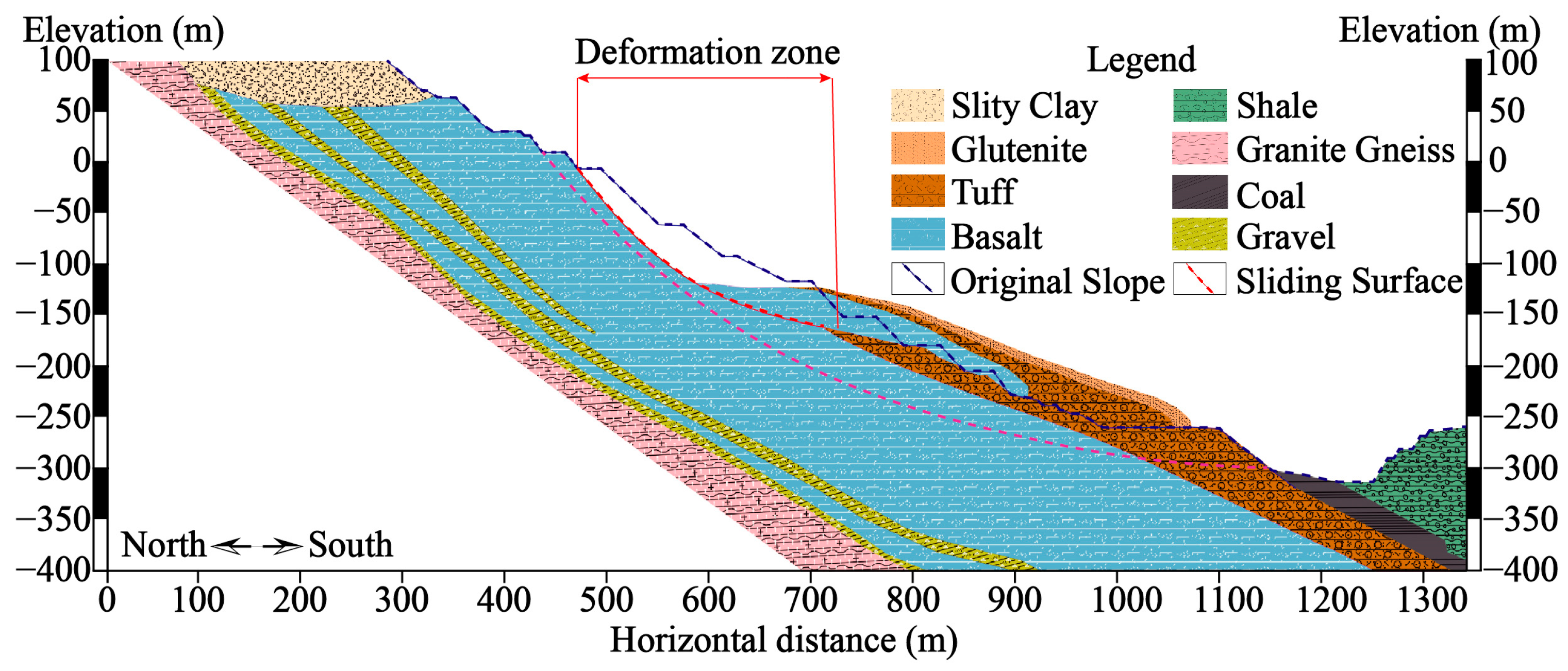
2.2. Geological Setting

By studying the exploration data of the initial mining area, along with a large volume of geological exploration information and conducting geological surveys, the rock masses of the slopes in the Fushun West open-pit mine have been classified into various lithologies, including granite gneiss, basalt, coal, oil shale, tuff, green mudstone, and miscellaneous fill soil. The exposed strata, from the oldest to the youngest, mainly consist of Precambrian granite gneiss, Paleogene Paleocene Lao Hutai Formation, Lizigou Formation, Eocene Guchengzi Formation, Jijuntun Formation, and West Open-Pit Formation. Quaternary artificial deposits also exist in the area. A comprehensive stratigraphic column is shown in Figure 2, and a profile of the landslide area is presented in Figure 3.

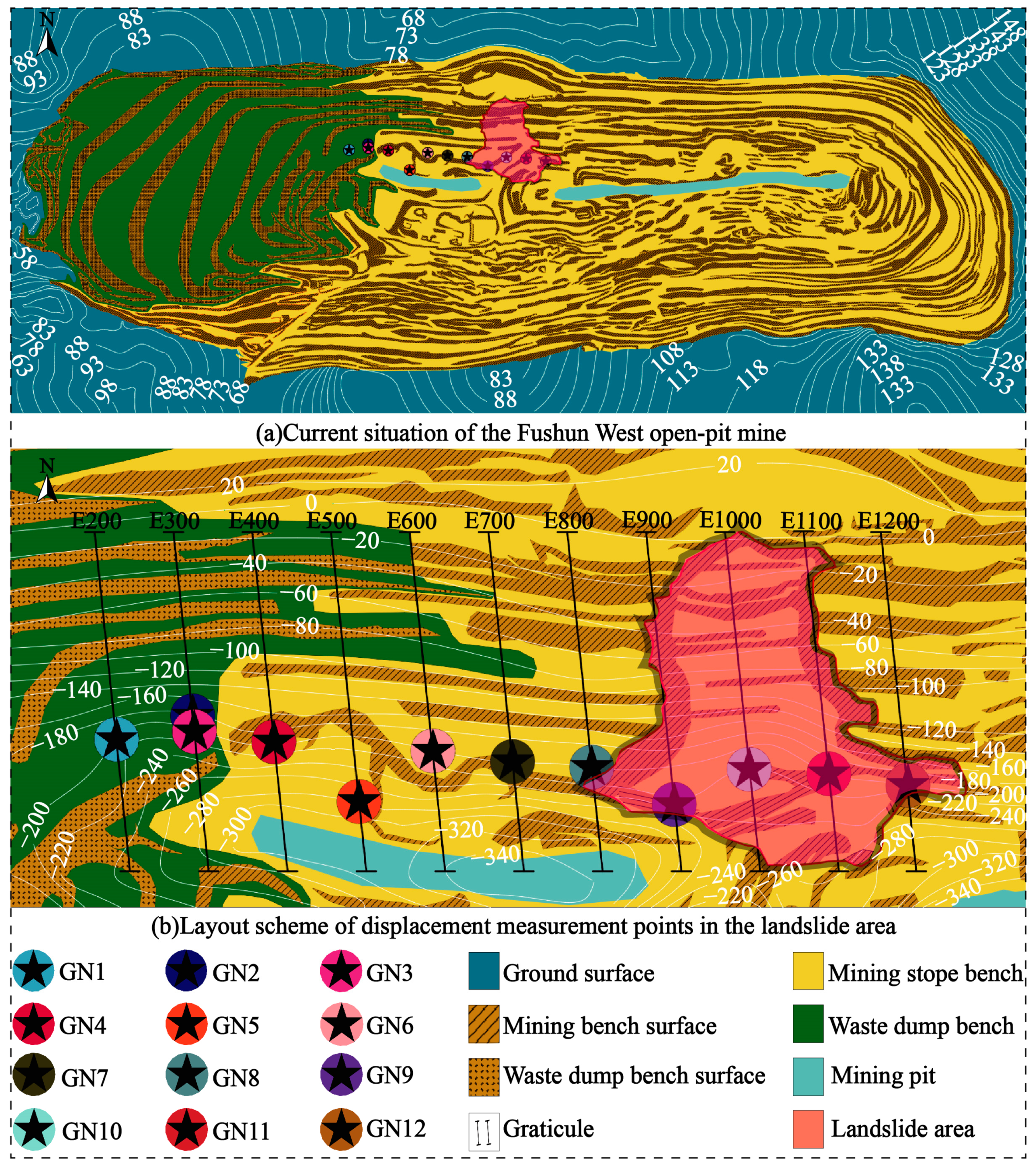
2.3. Data Description

GPS (Global Positioning System, hereafter called “GPS”) is a huge satellite-based system with global coverage for radio navigation and positioning. GPS technology has been developed rapidly in the application fields of navigation, positioning, precision measurement, etc. In particular, the GPS real-time monitoring system has been widely used in the field of real-time monitoring of landslide deformation in open-pit mines for its real-time nature, and has achieved better results.

In order to reduce the threat of landslide disasters in open-pit mines to national property and people’s lives, the Fushun West open-pit mine introduced a GPS real-time monitoring system, whose framework is shown in Figure 4. The system realizes the 24 h uninterrupted monitoring of geological disaster bodies and the remote automatic transmission of landslide displacement monitoring data, providing effective technical guarantees for the early warning of disaster bodies and the activation of emergency plans.

The system monitoring point deployment and GPS monitoring data are presented in detail below. A total of 11 monitoring profiles were established in different directions on the northern end slope of the Fushun West open-pit mine, Namely, E200, E300, E400, E500, E600, E700, E800, E900, E1000, E1100, and E1200. The engineering geological plan of the landslide is illustrated in Figure 5. As of June 2015, a total of 12 GPS monitoring points were deployed along the monitoring profile, as shown in Figure 5b. Its monitoring technology is mainly based on the main radar sensor transmitting microwaves, using differential aperture radar remote prism monitoring technology. The radar nominal precision is 0.1 mm, the frequency signal is 1575.42 Hz, and the wavelength is about 30~50 cm. These monitoring points were named GN1, GN2, GN3, GN, GN5, GN6, GN7, GN8, GN9, GN10, GN11, and GN12. For this study, data were selected from the period of 14 March 2016 to 31 August 2016.

Let the three-dimensional coordinate information of the landslide monitoring point at a certain time point acquired by remote prism synthetic aperture radar monitoring be (x, y, z). The 3D coordinate value corresponding to the initial moment t₀ is (x₀, y₀, z₀), the 3D coordinate value corresponding to any moment t_n is (x_n, y_n, z_n), and the cumulative displacement (Δx, Δy, Δz) component of the monitoring point within the moment from t₀ to t_t is:

$$\left\{\begin{array}{c}\Delta x=x_n-x_0\\ \Delta y=y_n-y_0\\ \Delta z=z_n-y_0\end{array}\right.$$

(1)

The change in total displacement $\Delta s$ at the monitoring point is:

$$\Delta s=\sqrt{\Delta x^2+\Delta y^2+\Delta z^2}$$

(2)

The cumulative displacement of the landslide is divided into cumulative horizontal displacement and cumulative vertical displacement, where cumulative vertical displacement is the cumulative displacement component in the z-direction and cumulative horizontal displacement Δh is:

$$\Delta h=\sqrt{\Delta x^2+\Delta y^2}$$

(3)

The direction of landslide sliding is indicated by the displacement azimuth, which is α:

$$\alpha =\arctan (\Delta x/\Delta y)$$

(4)

From the above definition, when α is positive, the displacement direction of the monitoring point is upward; when α is negative, the displacement direction of the monitoring point is downward. From the above derivation process, it can be seen that the size as well as the direction of the deformation of the landslide body is jointly determined by the magnitude of the x, y, and z directions. The deformation at any monitoring point on a landslide can be expressed in terms of the displacement components in the three directions of the monitoring point, or by horizontal displacement, vertical displacement, and displacement azimuth.

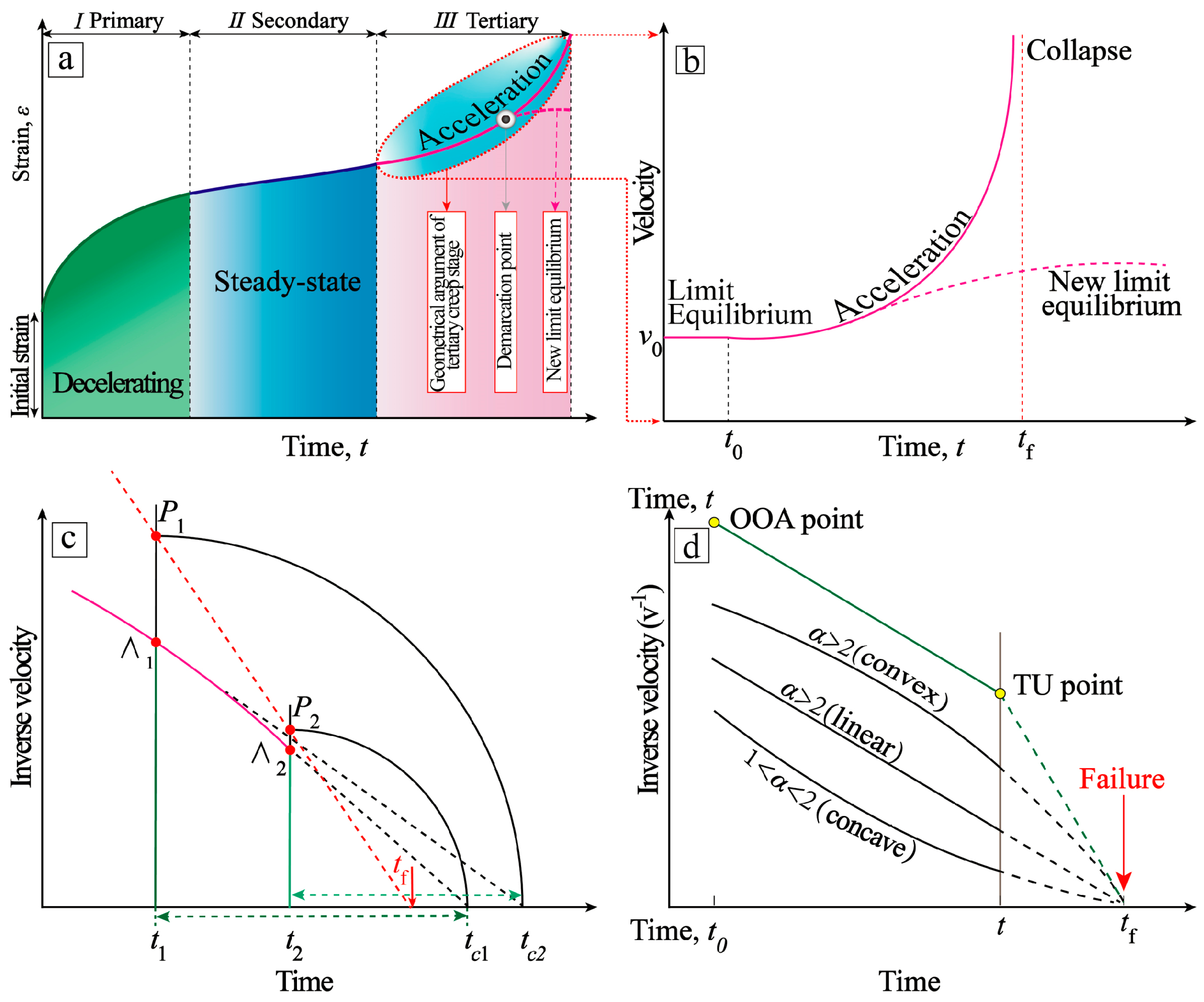
2.4. The Basal INV Method

The failure mechanism of slopes is defined as a complete paroxysmal collapse of rock and soil material. By analyzing a multitude of triaxial compression laboratory tests and in situ monitoring research, researchers have discovered that the deformation process of most landslides complies to the progressive characteristics [34,35,36] and three-stage law [37,38,39,40], as shown in Figure 6a. The whole process, from the initial deformation to the eventual failure, representatively comprises three stages: decelerating (green proportion), steady-state deformation (blue proportion), and acceleration deformation (pink proportion). Although the described methods have occasionally been successfully applied to a variety of cases such as man-made walls [30,41], rock and soil specimens [42,43,44], volcanic eruptions [45,46], or tunnels [45,47], these methods are primarily applied to unstable slopes. Hence, landslides are regarded as the principal research objects.

Fukuzono [21] further elaborated the classic three-stage creep theorem by propounding a simpler diagrammatic method (Figure 6b), which could be the most used and simple approach to provide a reasonable estimate of failure time. This method is valid for the tertiary stage. It is noteworthy that the method detects an OOA (onset of acceleration) point, which approximately distinguishes the secondary stage and the tertiary stage. The curve (Figure 6a) is separated into two segments by a demarcation point in the tertiary stage during the acceleration evolution process. (I) After an initial acceleration, Figure 6b displays a dotted line that is approximately parallel to the time axis with the landslide reaching equilibrium state; (II). Meanwhile, Figure 6b likewise displays a line whose value is towards ∞ (i.e., v⁻¹ → 0) as the velocity asymptotically increases.

Several authors successively supplied suggestions and guidelines for proficient usage based on a mathematical generalization of Fukuzono’s solution. Representatively, Voight [22,23] encompassed the prediction of failure behavior and proposed the following equation (Equation (5)).

$$d^2\mathsf{\Omega }/d^2{t}^2=\mathrm{A}(d\mathsf{\Omega }/dt{)}^{\alpha }$$

(5)

where Ω is the displacement, dΩ/dt and represents the “velocity” and “acceleration” of Ω, respectively. A and α are two empirical constants that denote characteristics of slope failure; recent investigations revealed that A and α are not independent of each other, varying with several factors comprising kinematic motion patterns [48], versatile types of materia, and macro or micro scales [49]. Consequently, Fukuzono proposed the following equation (Equation (6)) for predicting the failure time by combining the aforementioned equation (Equation (5)) with time:

$$\mathsf{\Lambda }\equiv v^{-1}={[A(\alpha -1)(t_f-t)]}^{{(\alpha -1)}^{-1}}$$

(6)

where t_f is the time of failure. This method consists in depicting a tangent line to the curve at an arbitrary point Ʌ₁ that tallies to moment t₁. The tangent passes across the horizontal axis at moment t_c1 (t_c1,0). Afterward, the point P₁ is plotted vertically above Ʌ₁, on a line that passes through Ʌ₁ and parallel to the Y axis. The segments of t₁Ʌ₁ and t₁t_c1 have an equal displacement from the perspective of geometric shapes. The abovementioned procedure is repeated for another random point Ʌ₂. Then, the time of failure t_f can be obtained as the abscissa of the intercept of a straight line that passes through P₁ and P₂ (Figure 6c).

The major drawback of Equation (5) is represented by the necessity of determining two constants A and α. According to closely controlled laboratory conditions and studies by several authors [50,51], α commonly spans over three orders of magnitude. For α = 2, 1 < α < 2, and α > 2, the curve of inverse-velocity has a linear, concave, or convex shape (Figure 6d), respectively. For this condition, Segalini et al. [52], who considered 26 emblematic pre-failure landslide cases, proposed that A inclines to take on extremely low or high values as α deviates from 2. While α appears as intermediate fluctuation, this attribute can be sufficient to sensibly influence prediction results.

To solve this issue, the value of α with the assumption that it is equal to 2 can be generally applied to evaluating the time of failure. In terms of guaranteeing production schedules and staff safety, the assumption of α = 2 is often integrated with the mining industry environment because of its demanding promotion of visual feedback. Thus, Equation (6) is simplified into the following equation (Equation (7)):

$$v^{-1}=A(t_f-t)$$

(7)

As a result, the failure time t_f is presumably provided for the point of abscissa of the extrapolated linear inverse velocity trend with the time axis.

2.5. The Moving Average Filtering INV Method Architecture

As formerly stated, the most powerful aspect of the INV method is probably its simplicity, and it is a useful resource in different instances, bypassing the intrinsic restriction for knowing the slope size, state of activity, and types of material. In addition, the tool resource also provides great convenience under many other aspects (e.g., risk assessment and management), if users can count on agile and suitable methods of appraising the state of the monitored circumstance and establish the probability of impending disastrous accidents, a task which is not always achievable because of hardly compensating restrictions as a consequence of measurement errors and random instrumental noise. Correspondingly, we verify two of the utmost prevalent and foolproof smoothing algorithms, i.e., finite impulse response models (also called moving average filter models). Three types of filter models are described below.

1. Short-term simple box filter (SSBF). As each new velocity datum sampling occurs, users can extract the unweighted mean of the antecedent data points through SSBF algorithm processing. This ensures that the alterations of v in the mean are coordinated with the alterations in the data (v) rather than being shifted in time. An example of a v simple equally weighted running mean is the mean over the latest k entries of a data set involving t entries. Let those velocity data points be v₁, v₂, …, v_t. The mean over the latest k velocity data points is represented as SSBF_k (${\overline{v}}_t$) and calculated as follows:

$$\begin{array}{l}{\overline{v}}_t=\frac{1}{m}(v_{t-k+1}+v_{t-k+2}\cdots v_t)\\ =\frac{1}{m}{\displaystyle \sum _{i=t-k+1}^t{v}_i}\end{array}$$

(8)

when the new velocity datum (SSBF_{k, next}, ${\overline{v}}_t^{\prime }$) is collected with the invariable sampling width m, the scope from t – k + 2 to t + 1 is considered. A new value v_t+1 comes into the sum and the earliest value v_t+1 drops out. This simplifies the computations by proceeding with the antecedent mean SSB_{Fk, antecedent}: (${\overline{v}}_t$)

$$\begin{array}{l}{\overline{v}}_t^{\prime }=1/k({\displaystyle \sum _{i=t-k+2}^{t+1}{v}_i})\\ =1/k(\underset{{\displaystyle \sum _{i=t-k+2}^{t+1}{v}_i}}{\underbrace{v_{t-k+2}+v_{t-k+3}+\cdots v_t+v_{t+1}}}+\underset{=0}{\underbrace{v_{t-k+1}-v_{t-k+1}}})\\ =1/k(\underset{={\overline{v}}_t^{\prime }}{\underbrace{v_{t-k+1}+v_{t-k+2}+\cdots v_t}})-\frac{v_{t-k+1}}{k}+\frac{v_{t+1}}{k}\\ ={\overline{v}}_t+\frac{1}{k}(p_{t+1}-p_{t-k+1})\end{array}$$

(9)

where the moving average cycle (k) of the SSBF model was set to 2 days (k = 2).

2. Long-term simple box filter (LSBF), where the moving average cycle (k) was selected to be 6 days (k = 6).

3. Exponentially weighted moving average (EWMA). Whereas in the short-term simple box filter (SSBF) and long-term simple box filter (LSBF), the past signal processing is weighted equally, the EWMA model is used to assign exponentially decreasing weights over time. The EWMA for a series can be calculated as follows:

$${\overline{v}}_t=\left\{\begin{array}{cc}{v}_0& t=0\\ \xi v_t+(1-\xi ){\overline{v}}_{t-1}& t>1\end{array}\right\}$$

(10)

where coefficient ξ represents the scale of recursion, a constant smoothing factor between 0 and 1. The smaller ξ is, the stronger the real-time performance of the moving average (${\overline{v}}_t$) is. On the contrary, the larger ξ is, the stronger the ability to absorb instantaneous burst value is, and the better the stability of the prediction model is. Hence, the smoothing factor with the assumption that ξ = 0.5 can be generally used to express and balance the recursion and attenuation properties of the prediction model.

Because the measurement instrument can be easily controlled by the geologist, the time interval between adjoining measurements can be given over a constant time interval. The pattern of filtering as in Equation (8) is equivalent to the easy mathematical statement utilized by Osansan and Stacey [52].

$$d{\mathsf{\Omega }}_i/d{t}_i=({\mathsf{\Omega }}_i-{\mathsf{\Omega }}_{i-n})/(t_i-t_{i-n})$$

(11)

In Equation (11), we set 1/Ω equal to 1/Ω_i (1/Ω_i is the reciprocal of displacement rate at t_i) and t equal to t_i (t₀ is the most recent instant).

The SSBF and LSBF models are customizable because they can be calculated for different numbers of time cycles (also called the order of the moving average). The biggest distinction of the SSBF and LSBF models is over setting the length of time cycles (k). Significantly, there is no regularly precise guideline or standard definition to set up the boundary between short-term and long-term cycles. It is noted that the selection of a suitable time cycle (k) value is due to the following two major elements: (i) monitoring data accuracy/quality; and (ii) data sampling frequency. To observe what the trend-cycle estimate looks like under different orders of moving average, we plot it (Figure 7) along with a group of monitoring data from an anonymous open-pit mine. It should be noted that the trend cycle (in red) is smoother than the original data after processing several moving averages (n < m < p < q) and captures the main movement of the time series without any of the minor fluctuations.

In Carlà et al. [30], the high-frequency rates of data acquisition, in the area of landslide monitoring programs, are representative of state-of-the-art radar monitoring technology (e.g., GPS [53,54], ground-based radar [31,55], total stations [56], and laser scanning [57]), and commonly require researchers to carry out smoothing over the bulk of measurements. Contrariwise, the low-frequency rates of data acquisition will produce low acquisition rates and will hide much of the background noise, resulting in the inability to trace short-term movements and delaying the identification of eventual trend changes; in such instances, smoothing should be performed over relatively lower measurements, compared to data obtained at high acquisition rates. Short-term averages respond quickly to changes in the price of the underlying security, while long-term averages are slower to react. The order of the moving average determines the smoothness of the trend-cycle estimate. In general, a large order means a smoother curve. The role played by the features of data sampling frequency and quality for the selection of suitable time cycles (k) is notable.

3. Results

3.1. Slope Displacement Velocity, Acceleration, and Cumulative Displacement Analysis

We collated the monitoring data with the period of 28 June 2016 to 31 August 2016, and plotted the velocity–acceleration–cumulative displacement curve of slope displacement, as shown in Figure 8. We divided the curve into three phases according to the trend of the velocity curve, i.e., the initial phase, the second phase, and the third phase. The phase splitting time points of the three phases of the different monitoring sites are not the same. The splitting time point of the first phase and the second phase is in the time interval from 12 July to 24 July, and the splitting time point jumps more, within 12 days, whereas the splitting time point of the second stage and the third stage is in the time interval from 9 August to 13 August, and the splitting time point jumps less; see the summary in

Table 1. Results of correlation analysis between vegetation and climate indicators.

Monitoring Point	The Initial Stage		The Second Stage		The Third Stage
	Start	End	Start	End	Start	End
GN1-E200-200	28 June	15 July	16 July	11 August	12 August	31 August
GN2-E300-184		12 July	13 July	10 August	11 August
GN3-E400-200		22 July	23 July	10 August	11 August
GN4-E400-188		21 July	22 July	10 August	11 August
GN5-E500-280		22 July	23 July	10 August	11 August
GN6-E500-200		24 July	25 July	10 August	11 August
GN7-E600-200		22 July	23 July	10 August	11 August
GN8-E700-200		18 July	19 July	10 August	11 August
GN9-E800-232		22 July	23 July	9 August	10 August
GN10-E900-220		22 July	23 July	12 August	13 August
GN11-E1000-200		16 July	17 July	11 August	12 August
GN12-E1200-200		14 July	15 July	11 August	12 August

for details.

As shown by the red curve in Figure 8, in the whole period, the overall velocity curve showed a downward trend and then an upward trend. In the first stage, the overall velocity curve showed a downward trend, but the downward trend was relatively gentle; in the second stage, the overall velocity curve showed a downward concave upward trend. In the third stage, the overall speed curve showed a trend of sharp rise and then a slow rise, and finally reached the highest point on 31 August. The time interval of the sharp rise of the curve in this stage was roughly distributed from 11 August to 15 August. In terms of numerical values, the velocity data of the monitoring points in the whole stage reached the highest point on 31 August, and the minimum velocity was measured by the monitoring point GN9 on 25 July, with a value of 17.00 cm/d. The maximum velocity, which was 83.50 cm/d, was measured by the monitoring point GN5 on 31 August. The velocity value span of GN4 was the smallest, ranging from 19.90 to 27.90 cm/d. The velocity value span of GN5 at the monitoring point was the largest, ranging from 27.00 to 83.50 cm/d.

As shown by the blue curve in Figure 8, in the first two stages, the acceleration curve fluctuates above and below 0, and the fluctuation range is the smallest in the whole stage. In the second stage, the acceleration curve is above 0 as a whole and shows an upward trend of fluctuation. The fluctuation range of the acceleration curve in the third stage is the largest in the whole stage, and the overall trend of fluctuation is decreasing. In terms of numerical value, the acceleration data of monitoring points in the whole stage reached the highest point on 14 August. The minimum absolute value of acceleration, which was −0.13 cm/d², was measured by the monitoring point GN11 on 13 July. The maximum acceleration, which was 4.30 cm/d², was measured by the monitoring point GN5 on 14 August. The acceleration value span of GN10 is the smallest, ranging from −0.2 to 0.65 cm/d². The acceleration value of GN5 at the monitoring point has the largest span, ranging from −0.2 to 4.30 cm/d².

As shown by the green curve in Figure 8, in the whole period, the cumulative displacement curve presents a linear upward trend. In the first stage, the cumulative displacement curve presents an upward convex trend. In the second stage, the cumulative displacement curve presents a linear upward trend. In the third stage, the cumulative displacement curve presents a linear downward concave upward trend. In terms of numerical value, the cumulative displacement data of monitoring points in the whole stage reached the highest point on 31 August. The minimum cumulative displacement, which was 105.19 cm, was measured by the monitoring point GN12 on 28 June. The maximum cumulative displacement was measured by the monitoring point GN5. On 31 August, the value was 234.99 cm. The cumulative displacement value span of GN9 is the smallest, ranging from 147.20 to 159.92 cm. The cumulative displacement value span of GN5 is the largest, ranging from 209.27 to 234.99 cm.

3.2. Analysis of Slope Displacement Inverse Velocity and Cumulative Displacement

According to the displacement–reverse velocity curve and the accumulated displacement curve drawn at 12 monitoring points, as shown in Figure 9 the trend of the reverse velocity curve mainly experienced three stages: slow acceleration, upward convex deceleration, and upward concave deceleration in the whole period. In the first stage, the reverse velocity curve showed an overall upward trend, but the upward trend was gentle. In the second stage, the inverse velocity curve presents an upward convex deceleration trend. The inverse velocity curve of the third stage showed an upward concave deceleration trend and finally reached its lowest point on 31 August. The time interval of the sharp downward trend of the curve at this stage was roughly distributed from 11 August to 15 August. In terms of numerical value, the inverse velocity data of monitoring points in the whole stage fell to the lowest point on 31 August. The minimum inverse velocity, which was 0.012, was measured by the monitoring point GN5 on 31 August. The maximum inverse velocity was measured by the monitoring point GN9 on 31 July, with a value of 0.059. The inverse velocity value span of GN4 is the smallest, ranging from 0.036 to 0.050. The inverse velocity value of GN8 has the largest span, ranging from 0.021 to 0.049.

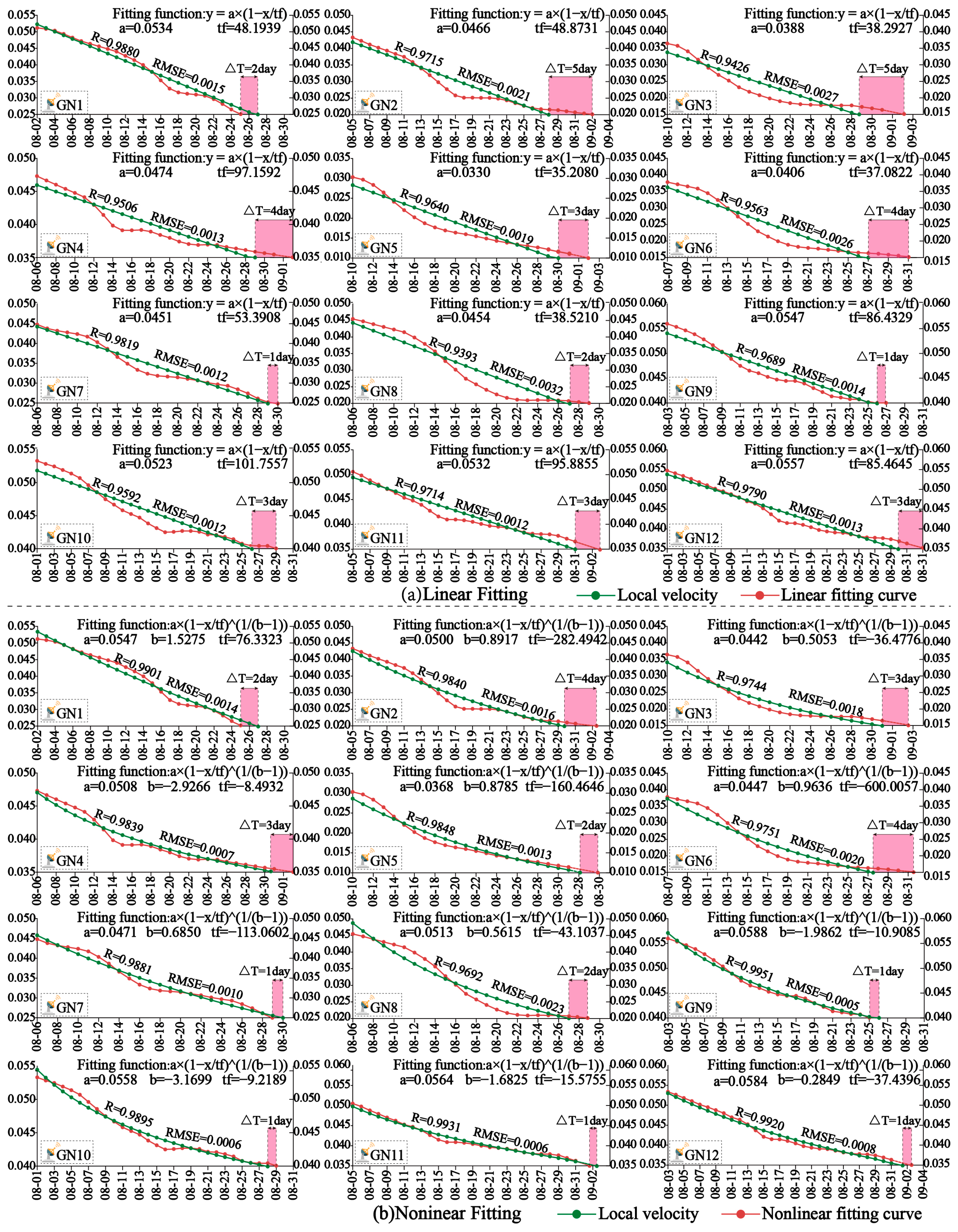
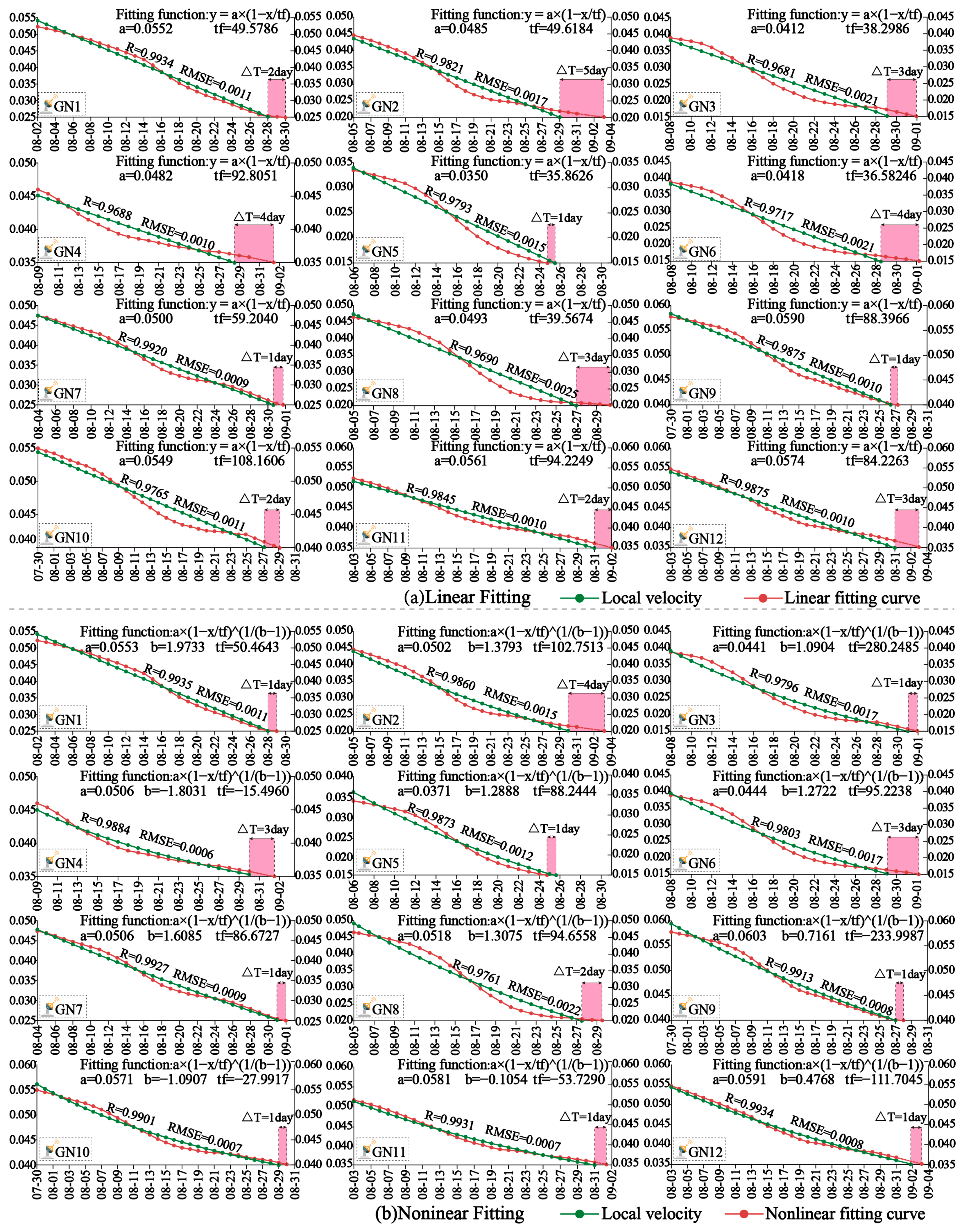
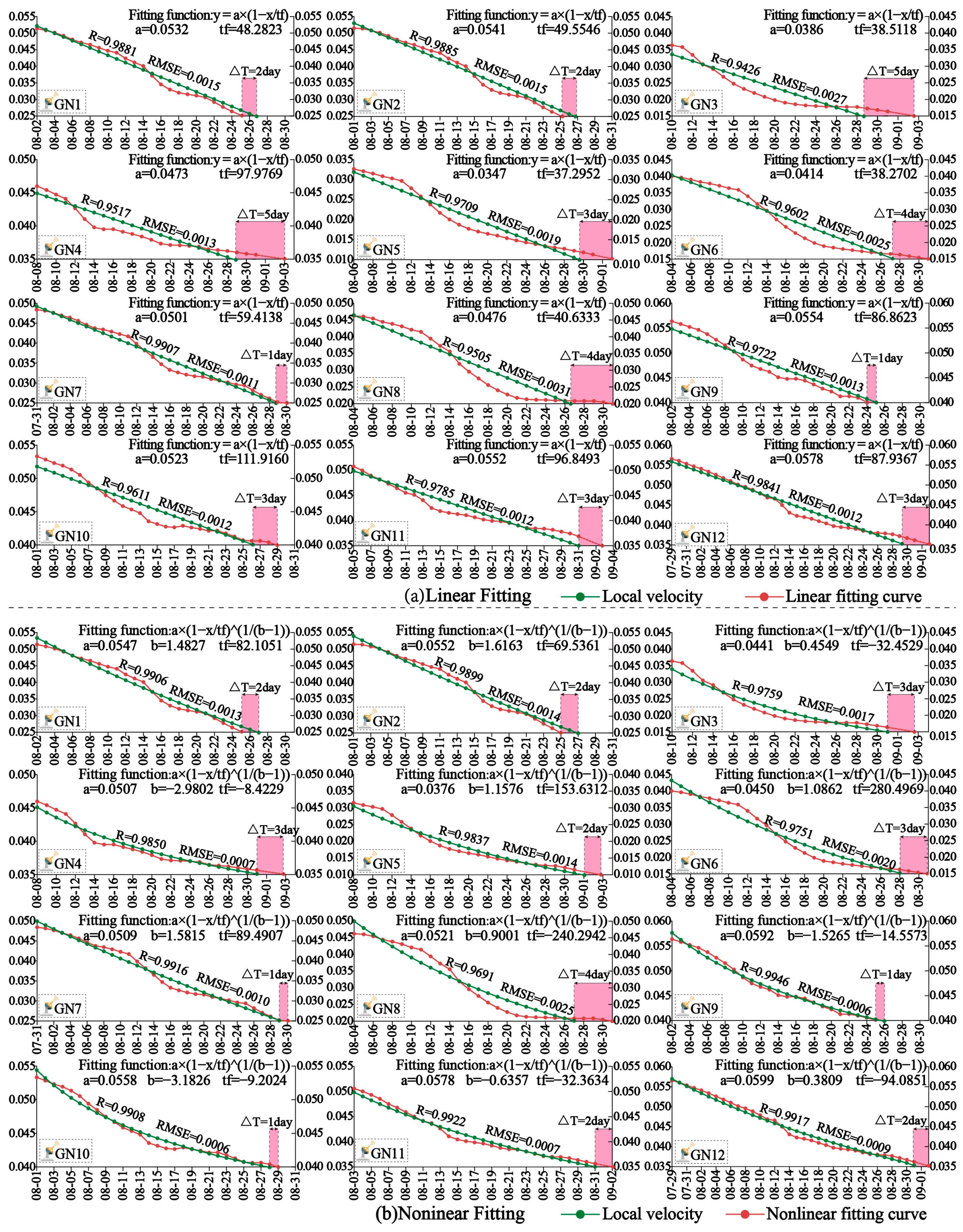
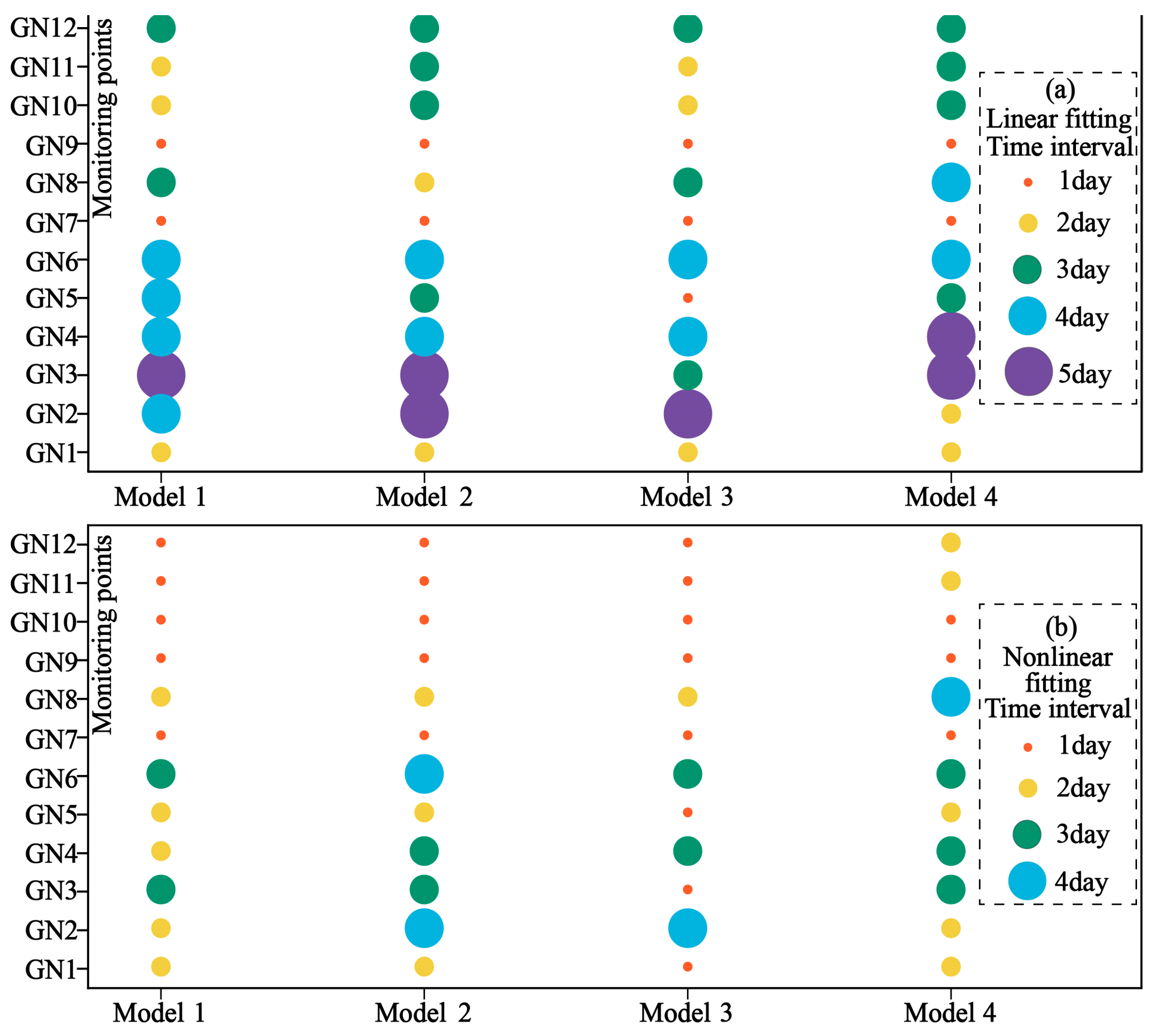
3.3. Source Velocity Data Model Analysis

The 12 monitoring points were transformed by the multiplicative inverse representation of velocity data under the time series model (as shown in Figure 10).

As shown in Figure 10, from 28 June 2016, the monitoring data acquisition starting point, the stage of large fluctuation ended on 31 August, and the period from 22 July to 31 August was the initial decay stage under the velocity multiplicative inverse representation. The curve trend of the 12 monitoring points is mainly presented as constant velocity attenuation–convex attenuation–concave attenuation–constant velocity attenuation. In terms of smoothness, this model is worse than other models. At the same time, since 11 August, the slope has completed the initial attenuation stage of large scale and also entered the next attenuation stage of relatively stable amplitude. At this stage, the amplitude of oscillation decreases compared with the initial attenuation stage. It is worth noting that under the representation mode of the multiplicative inverse meta-model of source velocity data, the curve shows obvious linear expression characteristics since 15 August. Linear and nonlinear fitting (as shown in Figure 10) was carried out for data under the multiplicative inverse meta-model of source velocity data. The landslide time predicted by 12 monitoring points is about 1–5 days earlier than the actual landslide time. Under the nonlinear fitting condition, the landslide time predicted by the 12 monitoring points under the model is about 1–3 days earlier than the actual landslide time, and the landslide time predicted by the GN1 and GN9 monitoring points under the model lags behind the actual landslide time by 2 days and 1 day, respectively. In terms of fitting effect and prediction effect, nonlinear fitting has better performance than linear fitting, and the overall prediction effect shows that the actual landslide time can be predicted in advance.

3.4. SMA Model Analysis

After the source velocity data were transformed by the multiplicative inverse representation of SMA model velocity data under the time series model (as shown in Figure 11), the stage of large oscillation amplitude ended on 31 August, and the period from 22 July to 31 August was the initial attenuation stage of SMA model. From the perspective of curve shape, the SMA model has an obvious tendency to eliminate the ladder shape of the curve based on the source velocity data model. Through the linear and nonlinear fitting of the data under the source velocity data SMA model, it can be obtained that under the linear fitting condition, the landslide time predicted by 12 monitoring points is about 1–5 days earlier than the actual landslide time. Under the nonlinear fitting condition, the landslide time predicted by the 12 monitoring points under the model is about 1–4 days earlier than the actual landslide time, and the landslide time predicted by the GN1 monitoring point is 2 days behind the actual landslide time. In terms of fitting effect and prediction effect, nonlinear fitting is better than linear fitting. The prediction effect of the SMA model is 1–2 days earlier than that of the multiplicative inverse model, but the overall prediction effect is worse than that of the multiplicative inverse model. The overall prediction effect is that the actual landslide time is predicted in advance.

3.5. LMA Model Analysis

After the source velocity data were transformed by the multiplicative inverse representation of the velocity data of the LMA model under the time series model (as shown in Figure 12), the stage of large oscillation amplitude ended on 31 August, and the period from 22 July to 31 August was the initial attenuation stage of the LMA model. From the perspective of curve shape, the LMA model further smoothed the curve shape based on the source velocity data model. The linear and nonlinear fitting of source velocity data under the LMA model showed that the fitting accuracy of the LMA model was the highest. Under the linear and nonlinear fitting conditions, the landslide time predicted by the model of 12 monitoring points is about 1–4 days earlier than the actual landslide time, and the landslide time predicted by the GN5 monitoring point is 1 day behind the actual landslide time. In terms of fitting effect and prediction effect, nonlinear fitting has a better performance than linear fitting. The landslide prediction time under the LMA model is 1–2 days shorter than that of the multiplication inverse model. The overall prediction effect is better than that of the multiplication inverse model, and the actual landslide time can be predicted in advance.

3.6. ESF Model Analysis

After the smooth velocity data were transformed by the multiplication inverse representation of the source velocity data under the time series model (as shown in Figure 13), the stage of large oscillation amplitude ended on 31 August. The period from 22 July to 31 August was the initial attenuation stage of the ESF model. In terms of curve morphology, the smoothness of ESF is better than that of the multiplicative inverse model but worse than the SMA model and LMA model. Under the linear fitting condition, the landslide time predicted by 12 monitoring points under the model is about 1–5 days earlier than the actual landslide time; under the nonlinear fitting condition, the landslide time predicted by 12 monitoring points under the model is about 1–3 days earlier than the actual landslide time. The predicted landslide time of the GN1, GN2, and GN9 monitoring points is 2 days, 2 days, and 1 day behind the actual landslide time, respectively. In terms of fitting effect and prediction effect, the nonlinear fitting has a better performance than the linear fitting. The landslide prediction time under the LMA model is 1–2 days longer than that under the multiplication inverse model. The overall prediction effect is worse than that of the multiplication inverse model, and the actual landslide time can be predicted in advance.

4. Discussion

The bubble chart between the actual landslide and the predicted landslide time is drawn in Figure 14. It can be seen from the figure that all four models can effectively predict the landslide in advance. Under the condition of linear fitting, the interval between the prediction time and the landslide time is guaranteed to be within 5 days. Under the nonlinear fitting condition, the interval between the prediction time and landslide time is guaranteed to be within 4 days, whereas the monitoring data of GN1, GN9, GN10, GN11, and GN12 shorten the interval between the prediction time and landslide time to within 2 days. In terms of fitting accuracy, the multiplicative inverse meta-model (model 1) is the lowest among the four models, followed by the ESF model (model 4); the SMA model (model 2) is better, and the LMA (model 3) model is the best. In terms of prediction accuracy, from the perspective of bubble size and distribution, ESF is the lowest among the four models, followed by the SMA model; the multiplicative inverse meta-model is better, and the LMA model is the best.

5. Conclusions

In this paper, based on the inverse velocity (INV) method of displacement monitoring data analysis, we examined the velocity time series by using four filters and comparatively analyzed the effect of landslide damage time prediction to improve the reliability of landslide prediction. The main conclusions of this study include the following points:

(1)

A landslide event comprises a rather complicated process. The results show that the sliding process of a landslide can be divided into three stages based on the INV: the initial attenuation stage (regressive stage), the second attenuation stage (progressive stage), and the linear reduction stage (autoregressive stage).

(2)

Compared with the raw data and the exponential smoothing filter (ESF) models, the fitting effect of short-term smoothing filter (SSF) and long-term smoothing filter (LSF) in the linear autoregressive stage is better.

(3)

In terms of fitting accuracy, among the four models proposed in this study, the fitting accuracy of the multiplicative inverse model is the lowest, followed by the ESF model; the SMA model is better, and the LMA model is the best. In terms of prediction accuracy, ESF is the lowest among the four models, followed by the SMA model; the multiplicative inverse model is better, and the LMA model is the best.

References

1. Tarolli, P.; Sofia, G. Human topographic signatures and derived geomorphic processes across landscapes. Geomorphology 2016, 255, 140–161. [Google Scholar] [CrossRef]
2. López-Vinielles, J.; Ezquerro, P.; Fernández-Merodo, J.A.; Béjar-Pizarro, M.; Monserrat, O.; Barra, A.; Blanco, P.; García-Robles, J.; Filatov, A.; García-Davalillo, J.C.; et al. Remote analysis of an open-pit slope failure: Las Cruces case study, Spain. Landslides 2020, 17, 2173–2188. [Google Scholar] [CrossRef]
3. Chen, J.P.; Li, K.; Chang, K.J.; Sofia, G.L.; Tarolli, P. Open-pit mining geomorphic feature characterisation. Int. J. Appl. Earth Obs. Geoinf. 2015, 42, 76–86. [Google Scholar] [CrossRef]
4. Paradella, W.R.; Ferretti, A.; Mura, J.C.; Colombo, D.; Gama, F.F.; Tamburini, A.; Santos, A.R.; Novali, F.; Galo, M.; Camargo, P.O.; et al. Mapping surface deformation in open pit iron mines of Carajás Province (Amazon Region) using an integrated SAR analysis. Eng. Geol. 2015, 193, 61–78. [Google Scholar] [CrossRef]
5. Tao, Z.G.; Shu, Y.; Yang, X.J.; Peng, Y.Y.; Chen, Q.H.; Zhang, H.J. Physical model test study on shear strength characteristics of slope sliding surface in Nanfen open-pit mine. Int. J. Min. Sci. Technol. 2020, 30, 421–429. [Google Scholar] [CrossRef]
6. Hoek, E.; Read, J.; Karzulovic, A.; Chen, Z.Y. Rock slopes in civil and mining engineering. In Proceedings of the ISRM International Symposium, Melbourne, Australia, 19–24 November 2000. [Google Scholar]
7. Bye, A.R.; Bell, F.G. Stability assessment and slope design at Sandsloot open pit, South Africa. Int. J. Rock. Mech. Min. 2001, 38, 449–466. [Google Scholar] [CrossRef]
8. Obregon, C.; Mitri, H. Probabilistic approach for open pit bench slope stability analysis—A mine case study. Int. J. Min. Sci. Technol. 2019, 29, 629–640. [Google Scholar] [CrossRef]
9. Carlà, T.; Farina, P.; Intrieri, E.; Botsialas, K.; Casagli, N. On the monitoring and early-warning of brittle slope failures in hard rock masses: Examples from an open-pit mine. Eng. Geol. 2017, 228, 71–81. [Google Scholar] [CrossRef]
10. Ma, K.; Sun, X.Y.; Zhang, Z.H.; Hu, J.; Wang, Z.R. Intelligent Location of Microseismic Events Based on a Fully Convolutional Neural Network (FCNN). Rock. Mech. Rock. Eng. 2022, 55, 4801–4817. [Google Scholar] [CrossRef]
11. Ma, K.; Yuan, F.Z.; Zhuang, D.Y.; Li, Q.S.; Wang, Z.W. Study on Rules of Fault Stress Variation Based on Microseismic Monitoring and Numerical Simulation at the Working Face in the Dongjiahe Coal Mine. Shock. Vib. 2019, 2019, 7042934. [Google Scholar] [CrossRef]
12. Zhang, Z.H.; Ma, K.; Li, H.; He, Z.L. Microscopic Investigation of Rock Direct Tensile Failure Based on Statistical Analysis of Acoustic Emission Waveforms. Rock. Mech. Rock. Eng. 2022, 55, 2445–2458. [Google Scholar] [CrossRef]
13. Crozier, M.J. Deciphering the effect of climate change on landslide activity: A review. Geomorphology 2010, 124, 260–267. [Google Scholar] [CrossRef]
14. Carlà, T.; Nolesini, T.; Solari, L.; Rivolta, C.; Dei Cas, L.; Casagli, N. Rockfall forecasting and risk management along a major transportation corridor in the Alps through ground-based radar interferometry. Landslides 2019, 16, 1425–1435. [Google Scholar] [CrossRef]
15. Liu, Z.J.; Qiu, H.J.; Ma, S.Y.; Yang, D.D.; Pei, Y.Q.; Du, C.; Sun, H.S.; Hu, S.; Zhu, Y.R. Surface displacement and topographic change analysis of the Changhe landslide on 14 September 2019, China. Landslides 2021, 18, 1471–1483. [Google Scholar] [CrossRef]
16. Intrieri, E.; Carlà, T.; Gigli, G. Forecasting the time of failure of landslides at slope-scale: A literature review. Earth Sci. Rev. 2019, 193, 333–349. [Google Scholar] [CrossRef]
17. Main, L.G. Applicability of time-to-failure analysis to accelerated strain before earthquakes and volcanic eruptions. Geophys. J. Int. 1999, 139, F1–F6. [Google Scholar] [CrossRef]
18. Tavenas, F.L.S. Creep and failure of slopes in clays. Can. Geotech. J. 1981, 18, 106–120. [Google Scholar] [CrossRef]
19. Dick, G.J.; Eberhardt, E.; Cabrejo-Liévano, A.G.; Stead, D.; Rose, N.D. Development of an early-warning time-of-failure analysis methodology for open-pit mine slopes utilizing ground-based slope stability radar monitoring data. Can. Geotech. J. 2015, 52, 515–529. [Google Scholar] [CrossRef]
20. Saito, M. Forecasting the time of occurrence of a slope failure. In Proceedings of the 6th International Mechanics and Foundation Engineering, Montreal, QC, Canada, 8–15 September 1965; pp. 537–541. [Google Scholar]
21. Fukuzono, T. A method to predict the time of slope failure caused by rainfall using theinverse number of velocity of surface displacement. Landslides 1985, 22, 8–13. [Google Scholar] [CrossRef] [PubMed]
22. Voight, B. A method for prediction of volcanic eruptions. Nature 1988, 332, 125–130. [Google Scholar] [CrossRef]
23. Voight, B. Materials science law applies to time forecasts of slope failure. Landslide News 1989, 3, 8–10. [Google Scholar]
24. Rose, N.D.; Hungr, O. Forecasting potential rock slope failure in open pit mines using the inverse-velocity method. Int. J. Rock. Mech. Min. Sci. 2007, 44, 308–320. [Google Scholar] [CrossRef]
25. Federico, A.; Popescu, M.; Elia, G.; Fidelibus, C.; Internò, G.; Murianni, A. Prediction of time to slope failure: A general framework. Environ. Earth Sci. 2012, 66, 245–256. [Google Scholar] [CrossRef]
26. Dick, G.J.; Eberhardt, E.; Stead, D.; Rose, N.D. Early detection of impending slope failure in open pit mines using spatial and temporal analysis of real aperture radar measurements. In Proceedings of the Slope 2013: 2013 International Symposium on Slope Stability in Open Pit Mining and Civil Engineering, Perth, Australia, 25 September 2013; pp. 949–962. [Google Scholar]
27. Newcomen, W.; Dick, G. An update to the strain-based approach to pit wall failure prediction, and a justification for slope monitoring. J. S. Afr. Inst. Min. Metall. 2016, 116, 379–385. [Google Scholar] [CrossRef]
28. Ma, H.T.; Zhang, Y.H.; Yu, Z.X. Research on the identification of acceleration starting point in inverse velocity method and the prediction of sliding time. Chin. J. Rock. Mech. Eng. 2021, 40, 355–364. [Google Scholar] [CrossRef]
29. Mufundirwa, A.; Fujii, Y.; Kodama, J. A new practical method for prediction of geomechanical failure-time. Int. J. Rock. Mech. Min. 2010, 47, 1079–1090. [Google Scholar] [CrossRef]
30. Carlà, T.; Intrieri, E.; Di Traglia, F.; Nolesini, T.; Gigli, G.; Casagli, N. Guidelines on the use of inverse velocity method as a tool for setting alarm thresholds and forecasting landslides and structure collapses. Landslides 2017, 14, 517–534. [Google Scholar] [CrossRef]
31. Carlà, T.; Farina, P.; Intrieri, E.; Ketizmen, H.; Casagli, N. Integration of ground-based radar and satellite InSAR data for the analysis of an unexpected slope failure in an open-pit mine. Eng. Geol. 2018, 235, 39–52. [Google Scholar] [CrossRef]
32. Zhou, X.P.; Liu, L.J.; Xu, C. A modified inverse-velocity method for predicting the failure time of landslides. Eng. Geol. 2020, 268, 105521. [Google Scholar] [CrossRef]
33. Chen, M.X.; Jiang, Q.H. An early warning system integrating time-of-failure analysis and alert procedure for slope failures. Eng. Geol. 2020, 272, 105629. [Google Scholar] [CrossRef]
34. Chandler, R.J. Recent European experience of landslides in over-consolidated clays and soft rocks. In Proceedings of the 4th International Symposium on Landslide, Toronto, ON, Canada, 16–21 September 1984; pp. 61–81. [Google Scholar]
35. Petley, D.N.; Higuchi, T.; Petley, D.J.; Bulmer, M.H.; Carey, J. Development of progressive landslide failure in cohesive materials. Geology 2005, 33, 201–204. [Google Scholar] [CrossRef]
36. Troncone, A.; Conte, E.; Donato, A. Two and three-dimensional numerical analysis of the progressive failure that occurred in an excavation-induced landslide. Eng. Geol. 2014, 183, 265–275. [Google Scholar] [CrossRef]
37. Main, L.G. A damage mechanics model for power-law creep and earthquake aftershock and foreshock sequences. Geophys. J. Int. 2000, 142, 151–161. [Google Scholar] [CrossRef]
38. Xu, Q. Theoretical studies on prediction of landslides using slope deformation process data (in Chinese with English abstract). J. Eng. Geol. 2012, 1020, 145–151. [Google Scholar]
39. Dixon, N.; Smith, A.; Flint, J.A.; Khanna, R.; Clark, B.; Andjelkovic, M. An acoustic emission landslide early warning system for communities in low-income and middle-income countries. Landslides 2018, 15, 1631–1644. [Google Scholar] [CrossRef]
40. Wang, X.G.; Yin, Y.P.; Wang, J.D.; Lian, B.Q.; Qiu, H.J.; Gu, T.F. A nonstationary parameter model for the sandstone creep tests. Landslides 2018, 15, 1377–1389. [Google Scholar] [CrossRef]
41. Bozzano, F.; Mazzanti, P.; Moretto, S. Discussion to: Guidelines on the use of inverse velocity method as a tool for setting alarm thresholds and forecasting landslides and structure collapses’ by T. Carlà, E. Intrieri, F. Di Traglia, T. Nolesini, G. Gigli and N. Casagli. Landslides 2018, 15, 1437–1441. [Google Scholar] [CrossRef]
42. Hao, S.W.; Liu, C.; Lu, C.S.; Elsworth, D. A relation to predict the failure of materials and potential application to volcanic eruptions and landslides. Sci. Rep. 2016, 6, 27877. [Google Scholar] [CrossRef]
43. Du, H.; Song, D.Q.; Chen, Z.; Guo, Z.Z. Experimental study of the influence of structural planes on the mechanical properties of sandstone specimens under cyclic dynamic disturbance. Energy Sci. Eng. 2020, 8, 4043–4063. [Google Scholar] [CrossRef]
44. Huang, J.; Liu, X.L.; Zhao, J.; Wang, E.Z.; Wang, S.J. Propagation of stress waves through fully saturated rock joint under undrained conditions and dynamic response characteristics of filling liquid. Rock. Mech. Rock. Eng. 2020, 53, 3637–3655. [Google Scholar] [CrossRef]
45. Kilburn, C.R.J. Forecasting volcanic eruptions: Beyond the failure forecast method. Front. Earth Sci. 2018, 6, 133. [Google Scholar] [CrossRef]
46. Dempsey, D.E.; Cronin, S.J.; Mei, S.; Kempa-Liehr, A.W. Automatic precursor recognition and real-time forecasting of sudden explosive volcanic eruptions at Whakaari, New Zealand. Nat. Commun. 2020, 11, 3562. [Google Scholar] [CrossRef]
47. Xu, C.; Liu, X.L.; Wang, E.Z.; Wang, S.J. Prediction of tunnel boring machine operating parameters using various machine learning algorithms. Tunn. Undergr. Space Technol. 2021, 109, 103699. [Google Scholar] [CrossRef]
48. Petley, D. Global patterns of loss of life from landslides. Geology 2012, 40, 927–930. [Google Scholar] [CrossRef]
49. Terzaghi, K. Mechanism of Landslides. In Application of Geology to Engineering Practice; Paige, S., Ed.; Geological Society of America: Boulder, CO, USA, 1950. [Google Scholar] [CrossRef]
50. Bozzano, F.; Cipriani, I.; Mazzanti, P.; Prestininzi, A. A field experiment for calibrating landslide time-of-failure prediction functions. Int. J. Rock Mech. Min. Sci. 2014, 67, 69–77. [Google Scholar] [CrossRef]
51. Segalini, A.; Valletta, A.; Carri, A. Landslide time-of-failure forecast and alert threshold assessment: A generalized criterion. Eng. Geol. 2018, 245, 72–80. [Google Scholar] [CrossRef]
52. Osasan, K.S.; Stacey, T.R. Automatic prediction of time to failure of open pit mine slopes based on radar monitoring and inverse velocity method. Int. J. Min. Sci. Technol. 2014, 24, 275–280. [Google Scholar] [CrossRef]
53. Benoit, L.; Briole, P.; Martin, O.; Thom, C.; Malet, J.P.; Ulrich, P. Monitoring landslide displacements with the Geocube wireless network of low-cost GPS. Eng. Geol. 2015, 195, 111–121. [Google Scholar] [CrossRef]
54. Samodra, G.; Ramadhan, M.F.; Sartohadi, J.; Setiawan, M.A.; Christanto, N.; Sukmawijaya, A. Characterization of displacement and internal structure of landslides from multitemporal UAV and ERT imaging. Landslides 2020, 17, 2455–2468. [Google Scholar] [CrossRef]
55. Chae, B.G.; Park, H.J.; Catani, F.; Simoni, A.; Berti, M. Landslide prediction, monitoring and early warning: A concise review of state-of-the-art. Geosci. J. 2017, 21, 1033–1070. [Google Scholar] [CrossRef]
56. Pecoraro, G.; Calvello, M.; Piciullo, L. Monitoring strategies for local landslide early warning systems. Landslides 2019, 16, 213–231. [Google Scholar] [CrossRef]
57. Abdulwahid, W.M.; Pradhan, B. Landslide vulnerability and risk assessment for multi-hazard scenarios using airborne laser scanning data (LiDAR). Landslides 2017, 14, 1057–1076. [Google Scholar] [CrossRef]
Figure 1. Location of the study area and geomorphology of the open-pit mine: (a) Location map of the Fushun West open-pit mine; (b) aerial view of landslide form.
Water 16 00430 g001
Figure 2. Lithology of the typical borehole.
Water 16 00430 g002
Figure 3. Section view of the landslide area.
Water 16 00430 g003
Figure 4. GPS monitoring system framework for the Fushun West open-pit mine.
Water 16 00430 g004
Figure 5. Landform and diagram of the open-pit mine landslide: (a) current situation of the open-pit mine; (b) layout scheme of displacement measurement points in the landslide area.
Water 16 00430 g005
Figure 6. Conventional three-stage interpretation of creep behavior. (a) Three-stage deformation process of the progressive landslide (modified after Saito, [20]); (b) kinematic evolution of a landslide (modified after Intrieri et al. [16]); (c) graphical approach for determining the time of failure in the tertiary creep stage (Intrieri et al. [16]); and (d) schematic diagram of INV (modified after Fukuzono, [21]).
Water 16 00430 g006
Figure 7. Different orders of moving average applied to displacement rates in an anonymous open-pit mine of the instability before the failure. n, m, p, and q represent the four order values of successive increments (i.e., n < m < p < q). (a) Displacement rate at successive incremental order values of n; (b) Displacement rate at successive incremental order values of m; (c) Displacement rate at successive incremental order values of p; (d) Displacement rate at successive incremental order values of q.
Water 16 00430 g007
Figure 8. Slope displacement velocity, acceleration, and cumulative displacement curve.
Water 16 00430 g008
Figure 9. Slope displacement inverse velocity and cumulative displacement curve.
Water 16 00430 g009
Figure 10. Source velocity data model analysis curve.
Water 16 00430 g010
Figure 11. SMA model analysis curve.
Water 16 00430 g011
Figure 12. LMA model analysis curve.
Water 16 00430 g012
Figure 13. ESF model analysis curve.
Water 16 00430 g013
Figure 14. Evaluation of model prediction accuracy.
Water 16 00430 g014