
Study of the River Discharge Alteration

1
Faculty of Civil Engineering, Transilvania University of Brașov, 900152 Brașov, Romania
2
Faculty of Civil Engineering, Bauhaus-Universität Weimar, 99423 Weimar, Germany
*
Author to whom correspondence should be addressed.
Water 2024, 16(6), 808; https://doi.org/10.3390/w16060808
Submission received: 21 January 2024
/
Revised: 5 March 2024
/
Accepted: 7 March 2024
/
Published: 8 March 2024
(This article belongs to the Special Issue Water Resource Management: Hydrological Modelling, Hydrological Cycles, and Hydrological Prediction)
Abstract
:This article aims to analyze the alteration in water discharge due to the building of one of the largest dams in Romania. Modifications in the hydrological patterns of the studied river were emphasized by a complex technique that includes decomposition models of the series into trends, seasonal indices, and random components, as well as into Intrinsic Mode Functions (IMFs). The Mann–Kendall trend test indicates the existence of different positive slopes for the subseries S1 and S2 (before and after the inception of the Siriu dam, respectively) built from the raw series, S. The stationarity hypothesis was rejected for all series. The multifractal analysis shows two different patterns of the data series. After decomposing the subseries S1 and S2, it resulted that the seasonality indices are not the same. Moreover, the seasonal variations decreased after building the dam. Empirical Mode Decomposition (EMD) unveils different short- and long-term patterns of the series before and after building the dam, concluding that there is a significant alteration in the river discharge after the dam’s inception.
1. Introduction
River systems are lifelines that sustain ecological balance, support civilizations, and reflect the complex interplay between natural processes and human interventions. Ancient civilizations thrived along riverbanks, leveraging the waterways for sustenance, irrigation, and transportation. The river discharge dynamic is influenced by diverse factors, from climatic variations to anthropogenic alterations [1]. Infrastructural developments like dam-building can profoundly impact the natural river flows [2,3,4]. When dams interfere with flow regimes, it often results in significant environmental damage and biodiversity deterioration [5,6,7]. China’s Yangtze River’s Three Gorges Dam stands out as a testament to this influence, causing extensive alterations in river flow patterns. These changes have ripple effects, challenging ecosystems and posing notable dilemmas for local communities reliant on the river [8]. Significant river flow alterations have trapped sediments, modified the natural flow pattern, and disrupted the nutrient balances, affecting delta, estuarine, and marine ecosystems [9,10,11]. These ecological concerns emphasize the need for a balanced approach to infrastructural developments [12].
Despite the extensive studies on the dam’s impact on river flow and the environment, some gaps persist. One concerns the study of the cumulative impacts of smaller dams [13]. Although large dams have been the target of most research, the role of smaller dams has been emphasized recently [14]. Unlike mega-projects like the Three Gorges Dam which received extensive coverage, smaller dam projects need to be scrutinized more, leaving potential knowledge unknown [15]. Even if small dams might appear insignificant individually, their collective impact can be at least as potent as bigger dams, especially when it comes to flows that matter ecologically [14,15]. While the scientific literature contains numerous studies on this subject, a comprehensive critique is essential. There is a pressing need to examine how much dam constructions deviate river flows from their natural state, preserving intact ecological functions [16,17,18].
In pursuing a more holistic understanding, the research community has seen a convergence of conventional wisdom and innovative techniques for analyzing the rivers’ discharge. Given the urgent global imperative for sustainable water resource management, these research endeavors take on heightened significance [14]. As time evolved, the methodologies to study these dynamics expanded, including statistical analysis [19,20,21,22], wavelets decomposition [23], artificial intelligence methods—neural networks [24,25,26], support vector regression [27], time series models [28], hydrological simulation [29], etc.
IHA (Indicator of Hydrologic Alteration) [30] represents another tool to assess the hydrological alteration that is widely used by researchers [31,32,33,34,35,36,37,38]. The IHA software [30] can compute 33 flow statistical parameters divided into three classes—low, medium, and high—containing values less than or equal to the 33rd percentile, between the 33rd and the 67th percentiles, and above the 67th percentile, respectively. The software allows for the determination of the frequency of each annual post-impact value belonging to each category [37]. One main drawback is that many of these indices are intercorrelated [37], so the question is how many indicators are necessary to describe the river flow alteration. Other shortcomings are that no IHA directly quantifies the amplitude of high flow conditions, and no seasonality indices are provided. The latter are essential for understanding the seasons with high flows corresponding to possible floodings.
Within this complex realm, our research combines different approaches to cross-validate the results of the hydrological alteration in the Buzău River flow after operating the Siriu dam, Romania’s second biggest accumulation lake. Very few articles [38,39,40] have approached the impact of building the Siriu dam on the river flow, one of them using IHA [38] and the other [39] using statistical methods to test the existence of specific trends in seasonal series (winter, spring, summer, and autumn) before and after the dam’s inception. Another attempt was made by modeling the daily mean flow series using general regression neural networks (GRNNs) [40]. None of these studies have provided a complete analysis given that (1) assessing the tendency by the Mann–Kendall test followed by utilizing Sen’s slope (which computes a linear trend) [39] cannot capture the complex behavior of the data series (such as seasonality), (2) the linear parametric regression [38,40] was not satisfactory from the viewpoint of the extracted information, and (3) the GRNN model [40] was not accurate enough. In the GRNN, the correlation between the actual and predicted values on the test set was not very high, and the time taken to run the algorithm was very long (a few hours).
Our approach complements these procedures, providing seasonality indicators and emphasizing the flow pattern at short and long scales through Empirical Mode Decomposition (EMD), which offers granularity by breaking down intricate oscillatory patterns in river data [32]. The procedures utilized in the present study are easy to use and do not involve the computation and comparison of a high number of indicators, which can sometimes lead to confusing interpretations (as in IHA methods). Moreover, the time necessary to run the algorithms is extremely low (a few seconds) compared to the GRNN model.
The novelty of this research is that it introduces a unique framework that amalgamates the strengths of multifractal analysis with time series decomposition and EMD. The first one emphasizes the existence of periods with different behaviors of monthly river discharge series, the second provides the seasonality factors, and the last underscores the differences between the river’s short- and long-term variations before and after the dam’s construction. This combination gives a more nuanced view of the dam’s impact on Buzău discharge dynamics and clarifies the extent of the streamflow alteration.
2. Materials and Methods
2.1. Study Area
The Buzău River’s catchment, with a surface of 5264 km2 and an average elevation of 1043 m (Figure 1), is situated in the Romanian Curvature Carpathians. The climate of the study area is temperate–continental. From 1955 to 2010, the average (minimum) temperature was 6 °C (1 °C), the multiannual mean precipitation varied between 500 mm and 1000 mm [41], and the mean monthly precipitation (%) varied from 4.4 (in January) to 15 (in June and July).
The sub-basin catchment from where the River’s water is drained at Nehoiu is 1567 km2. The average river discharge ranges from 0.76 to 5000 m3/s, while the specific and multiannual averages are 17 L/s.km2 and 25.2 m3/s [42]. The Siriu dam, which can store up to 125 million m3 of water, was put in operation on 1 January 1984, on the Buzău River, upstream of Nehoiu. It drains about 56% of the water of this river and its tributaries [43] and supplies water to settlements and industrial plants downstream and for irrigating 50,000 ha [41].
Many catastrophic floods were recorded on the Buzău catchment after 1948, the biggest one in 1975, recording a maximum discharge of 2100 m3/s. One of the reasons that the dam was built was to avoid or at least diminish the effects of such events. Still, it does not protect the settlements downstream from floods produced by the Buzău’s tributaries (as in the case of flooding events in July 2004 and May 2005) [43]. In June–July 2010, a great flood affected many villages downstream of Nehoiu, damaging 14 pedestrian bridges and 1.2 km of water supplies and interrupting the communication between different villages.
2.2. Data Series
The studied series is formed by the monthly mean flow of the Buzău River measured at the Nehoiu station (45°25′29″ latitude and 26°18′27″ longitude) during January 1955–December 2010 (Figure 2).
The values of river discharge were measured daily at 7 a.m. and 7 p.m. and provided to the National Institute of Hydrology and Water Management (INGHA), where specialists checked them. The daily series were aggregated to obtain the monthly mean discharge. The dataset had no missing values.
To analyze the changes in water discharge after building the Siriu dam, the entire series, denoted by S, in the following, was split into two parts: S1—the series from January 1955 to December 1983 (before starting operating the Siriu dam), and S2—the series from January 1984 to December 2010 (after starting operating the Siriu dam). This split was performed to compare S1 and S2 and determine if the river discharge was altered due to the dam’s operation.
The mean values for S, S1, and S2 are 21.83, 23.15, and 20.41 m3/s, respectively. The maximum decreases significantly from 117.29—for S and S1—to 92.79 m3/s for S2. The highest variance is noticed for S1 (347.58) and the lowest for S2 (259.14). There is no significant difference between the series skewness, but the kurtosis decreases from 3.93 (for S and S1) to 3.43 for S2. So, all distributions are right-skewed and leptokurtic. The outliers of S and S1 are in the same range, but those of S2 have values lower than 100 m3/s, mostly under 70 m3/s. The histograms and boxplots are shown in Figure 3.
2.3. The Study Stages
This study introduces a complex framework to clarify the extent of Buzău River water discharge modifications after building the Siriu dam. The study’s flowchart is presented in Figure 4 and the detailed steps of the methodology are introduced below.
- Perform the statistical analysis to determine if there are common futures (trend or stationary) of S, S1, and S2. This includes the following:
- We rest the null hypothesis that there is no trend in the data series against the alternative of a monotonic trend existence using the Mann–Kendall (MK) [46] and seasonal Mann–Kendall (SMK) trend test [47]. Since there are n seasons, with m observations each, the null hypothesis in SMK is that observations are independent and identically distributed, and the alternative is that a monotonic trend is presented in the data series. First, a test statistic similar to the MK test’s is built for each season. Then, the MK statistic for the seasonal test is obtained by summing the n statistics. The decision is made to reject the null as in the MK test [48]. When the null hypothesis is rejected, the trend is determined by the non-parametric Sen’s method [49] as the median of the slopes of all of the pairs of ordinal time points.
- We test the series stationarity by following the KPSS [50] procedure. The null hypothesis is the series level or trend stationarity; the alternative is its non-stationarity. Testing this hypothesis is important for building forecast models for the studied series.
- Assess the existence of the different behaviors of the studied series on subintervals and emphasize their scaling characteristics through the multifractal analysis [51,52].It was shown [47,48] that if a time series exhibits scaling properties, its behavior can be expressed in an exponential form (1), with the mass exponent , which can be estimated by fitting a linear regression of log vs. logλ (λ > 0) [53]. So,where is the partition function, whose values can be computed by covering the series chart with a certain number of boxes of size and summing up the probabilities of the appearance of a gray value in a box [54].The multifractality can also be assessed by computing Renyi’s dimension, D(q) [55], whose relationship with is [56] as follows:The series presents multifractality if D(q) decreases when q increases. When D(q) has a constant value (equal to D(0)), the series is monofractal.An alternative way to characterize the multifractality is by using the f(α) spectrum, which is defined by the equationand can be computed by using a Legendre transform of in the following form:where is the Hölder exponent [57].In the multifractality case, the f(α)’s chart shape is single-humped.The steps in the MFDFA are [53] as follows:
- Compute the series cumulative sum, F.
- Split F into Ns subseries (each containing s values).
- Apply the least squared method for fitting an n-th order polynomial.
- Build the detrended F series by subtracting the polynomial values from the subseries’ values.
- Build the fluctuation function, Fq, by taking the q-th root of the mean of the square functions from the previous stage.
- Fit the function ~, with h(q) as the generalized Hurst exponent.
- Perform the time series decomposition to analyze the changes in the seasonality factors before and after the dam’s inauguration.The series () is decomposed into a trend (), seasonality (), and random noise component () using an additive model or multiplicative model. The best model is selected based on the smallest mean standard error (MSE), mean absolute error (MAE), or mean absolute percentage error (MAPE). So, the additive decomposition model—ADM (the multiplicative decomposition model—MDM)—will be calculated as follows:In this approach, the trend is computed by a moving average of the 12th order, and then, the deseasonalized series () is determined. The row seasonality indices are computed as averages of the values of each month. These final seasonality indices are calculated by adjusting the raw ones to add up to zero. The random component (residual) is the difference between the detrended series and the series obtained by replicating the 12 seasonality indexes for each year.In the case of the MDM, the deseasonalized series is computed by . The seasonality indices are obtained similarly to the ADM case, and the residual is obtained by dividing the deseasonalized series by the seasonality indices [58].
- Perform EMD to determine the short and long-term variations in S1 and S2 and detect the differences in their patterns.EMD is an adaptive data analysis technique of non-linear and non-stationary time series aiming to decompose the series into a collection of oscillatory components called IMFs [59,60]. The importance of this technique is given by the following characteristics [60,61,62]:
- Adaptability and Flexibility: Unlike other decomposition methods, which often impose predetermined basis functions (like sine and cosine functions in Fourier analysis), EMD does not rely on any a priori basis. This means it can adapt to the nature of the data and make the decomposition more accurate and meaningful.
- Local Characterization: EMD provides a local representation of data. Each IMF captures oscillations occurring over a specific time scale, crucial in analyzing data where different periodic components might overlap or where transient features (like spikes or dips) are of interest.
- Versatility: While initially developed for time series analysis, EMD has shown remarkable performance in various fields, including climatology, biomedical signal analysis, and financial market research.
- Handling Non-Linearity and Non-Stationarity: Most traditional methods fail or require stringent preprocessing when dealing with non-linear or non-stationary data. EMD is inherently suited for such data types, providing a robust decomposition even in challenging conditions.
- (a)
- Initialization: with the entire dataset, data(t), as the input, identify the sets of local maxima and minima and denote them by Max(t) and Min(t), respectively.
- (b)
- Building the envelope through interpolation:
- Use a cubic spline interpolation or any suitable method to generate the upper envelope by connecting all of the Max(t) points.
- Similarly, connect all of the Min(t) points to create the lower envelope.
- (c)
- Compute the mean envelope, m(t), by using the following equation:m(t) = (upper envelope + lower envelope)/2.
- (d)
- Extract the detail, h(t), by using the following equation:h(t) = data(t) − m(t).
- (e)
- Verify the Intrinsic Mode Function (IMF) criteria:
- Check if h(t) is an IMF, that is, by the following:
- ✓
- The number of extrema and zero-crossings must be equal or differ at most by one.
- ✓
- For any t, the mean value of the envelope defined by the local maxima (minima, respectively) is null.
- If h(t) is an IMF, go to (f); otherwise repeat the procedure from (b) using h(t) as input.
- (f)
- Perform iterations and compute the residual:
- For an identified IMF, h(t), subtract it from the original data and rename the resultant as the new data.
- Continue the new data-sifting process, extracting further IMFs.
- Continue the iteration until the residue becomes monotonic, showing no more IMFs can be extracted.
- (g)
- Compile the results:
- Collate all extracted IMFs.
- Record the final residue left after all possible IMFs have been derived. It should be a monotonic function.
This approach will underscore the differences in trend and seasonality of S1 and S2 and clarify the extent of the river flow alteration after operating the dam.
3. Results
3.1. Results of Statistical Analysis, Multifractal Analysis and Series Decomposition
Table 1 contains the results of the statistical tests on the data series performed at a significance level of 0.05. A p-value (computed in a test) less than 0.05 leads to the rejection of the respective null hypothesis.
The MK and SMK tests could not reject the randomness hypothesis for S. They rejected it when applied to S1 and S2 (Table 1, column 2, row 3). The trend values, computed by Sen’s method, are indicated inside the brackets and marked with * in Table 1. They are 0.0139 for S1 and 0.0311 for S2, so there is an increasing trend in the river discharge for both subseries, but not for the entire series. The result indicates that the trends of the subseries are different, indicating a different behavior of S1 and S2. Still, the slopes of the trends of S1 and S2 are very small, and putting together S1 and S2 (resulting in S) will not guarantee a significant trend for S. Indeed, the rejection of the null hypothesis for S shows that no significant trend was detected for it.
The stationarity hypothesis could not be rejected for all series. The results of the multifractal analysis are displayed in Figure 5.
The chart of the mass exponent (Figure 5a) presents two subseries for which two linear trend lines can be fitted—for q ∈ [−10, 0] and for q ∈ [0, 10]. The slope change is at zero, so the series has a multifractal character. The shape of the generalized Hurst’s exponent chart ( vs. q, Figure 5b) is a damped sine shape, with an inflection point at q = 0. In Figure 5c, one may notice deviations in the estimated segmentation function values from the linear trend (represented by straight lines in black, blue, and green, respectively). This variability is higher for q = 10, as the right-hand side of the chart shows the distribution of the function’s values (represented by rectangles) with a higher slope than its values situated at the chart’s right hand. The f(α) spectrum (Figure 5d) has a parabolic shape, indicating the series multifractality. The previous remark shows that the Buzău River’s flow series has a multifractal character. We may assume that it is the effect of the pattern change in the rivers’ discharge after building the dam.
The decomposition of the S series was performed to emphasize this change and find the seasonality components in particular. The elements in the ADM and MDM are presented in Figure 6 and Figure 7.
The raw series and the trend are the same but the seasonal and the residual components are different. The values of the seasonality indices are presented in Table 2. In both cases, the highest indices were registered in April and May and the lowest in January. In the case of the MDM, all indices are positive and vary in the interval [0.4986, 2.1326]. In the ADM, seven indices are negative, only five are positive, and the variation interval is [−10.700, 23.5093].
The positive indices correspond to the spring and summer months (March–July), indicating a higher impact of the seasonal variations on the water flow (more precipitation, and thus a higher flow, is recorded in spring and the beginning of summer). The residuals comparison shows a smaller amplitude for the MDM compared to the ADM, with a lower autocorrelation order (Figure 8a,c) and lower skewness and kurtosis (Figure 8b,d), respectively: 1.4351 compared to 1.5316, and 2.7742 compared to 5.2396.
The residuals’ MAE, MSE, and MAPE are 8.3273, 144.7643, and 50.5265 in the ADM and 0.9917, 1.2364, and 6.3449 in the MDM. Therefore, the best decomposition is provided by the second method. So, based on the MDM, similar seasonal variations are recorded in the last month of autumn and the first month of winter, being slightly higher in February and September and lower in January. The seasonal factor of 1.2012 in March might be explained by the snowmelt at the beginning of spring, and that from April to June is due to the high precipitation in spring.
The same analysis was performed for the subseries S1 and S2 to examine if there are significant differences between the seasonality factors. These indices in the MDMs are given in Table 3.
The seasonality indices’ pattern is similar to that in the MDM for S, with the highest values in April, May, June, and March or July and the lowest in January. The amplitude of the seasonality indices’ decreased from 1.6902 = 2.1553 − 0.4751 to 1.5835 = 2.1215 − 0.538, indicating an attenuation of the extreme events.
3.2. Cross-Validation of the Results Using EMD
EMD was finally applied to cross-validate the above findings. A set of plots was created to represent and analyze the data effectively. The initial step was to display the original data over time as scattered points, with the amplitude of monthly averages depicted through a color map. Subsequent plots showcased each computed IMF, with enhanced subplots for improved readability. Cubic spline interpolation was utilized to visualize each IMF in greater detail. Furthermore, residuals were also visualized individually and in combination with the IMFs to provide an all-encompassing view.
In data analysis, accurate and clear visualization is essential. Therefore, two methods were used to draw the IMFs: fine indexing and cubic spline interpolation. Fine indexing is similar to zooming into an image to see details. It increases the number of examined points, allowing for a more detailed view of data trends. Cubic spline interpolation uses polynomial functions to connect these points, creating a smoother curve. It ensures that the curve passes through the data points and transitions smoothly between them.
These two techniques provide a more detailed and smooth visualization, making data trends more evident. With more data points from fine indexing and smoother curves from interpolation, subtle patterns in the data can be more easily identified. Without these methods, data visualizations can appear disjointed, and some subtler patterns might be overlooked or misinterpreted.
Figure 9 contains details from visualizing IMF 3 and IMF 4 for S using the abovementioned techniques. In the first case, the interpolated IMF 3 passes through the original points of IMF 3. In the second one, the original IMF 4 is formed by points on parallel lines, and the interpolated IMF 4 provides a smooth image of the original one. Upon decomposing the data with EMD, several IMFs are obtained. Figure 10 shows eight of them in EMD for the S series.
The first IMF presents the highest frequency oscillations observed in the dataset, typically corresponding to short-term changes. The periods with high oscillations might correspond to the months when floods were recorded. These oscillations are still kept by IMF 2. IMFs 3 and 4 show long periods with similar behavior, followed by some peaks. IMFs 3–5 reveal a slightly lower frequency, indicating seasonal fluctuations. IMFs 6 and 7 show an almost perfect sine behavior, whereas IMF 8 has a decreasing trend. They display patterns that might be correlated with multiyear climate cycles or longer-term environmental changes. The remaining values are very low (of the order 10–15), signifying good series decomposition.
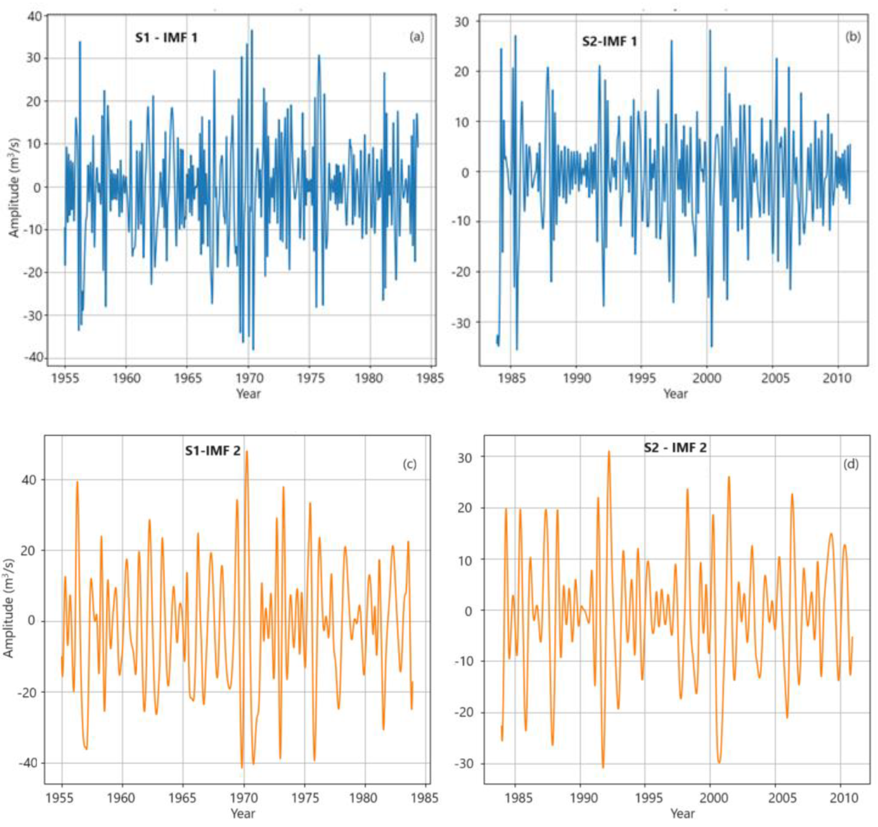
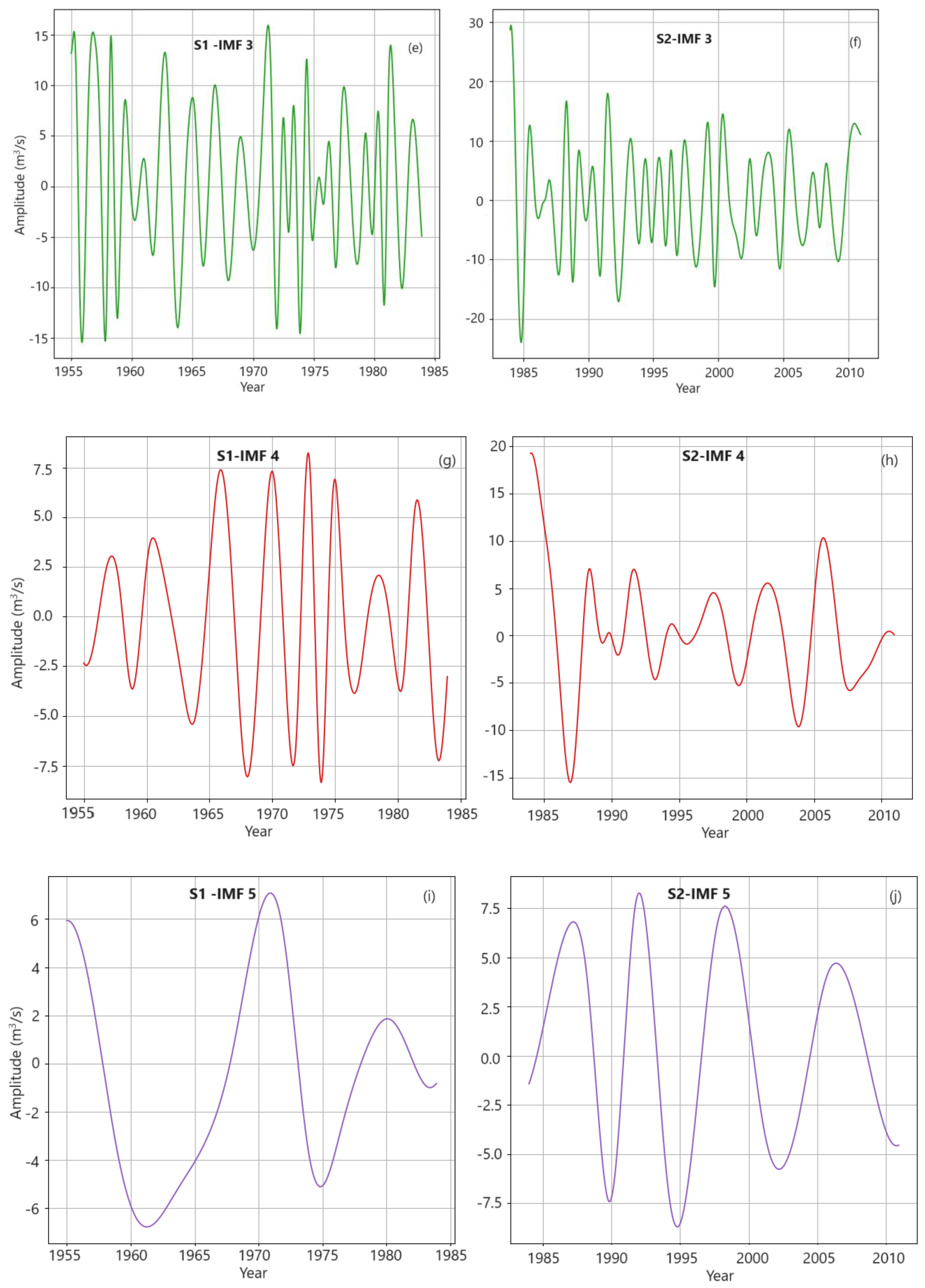
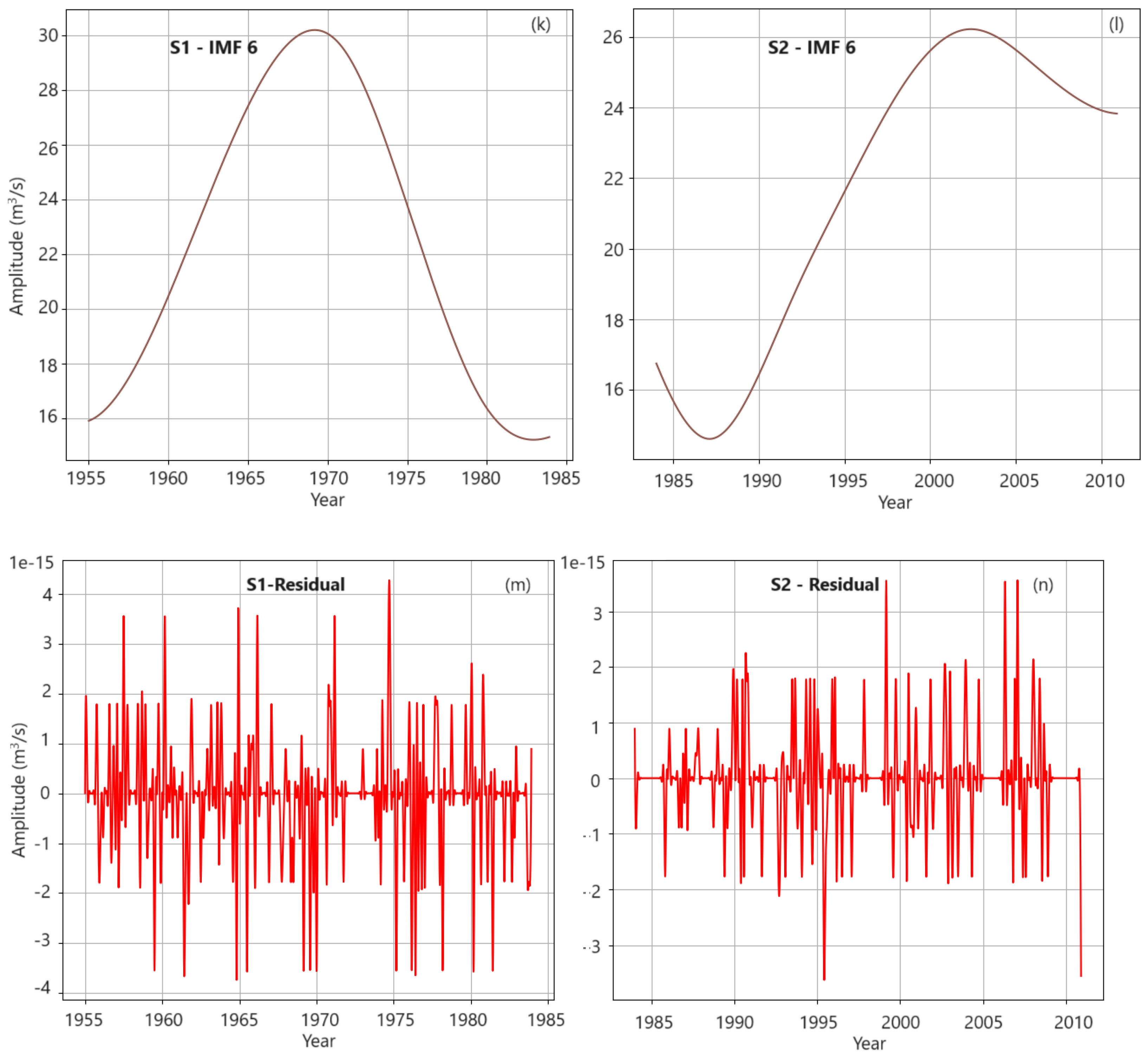
An additional investigation was carried out for S1 and S2 (Figure 11) to analyze any potential differences or anomalies in the discharge pattern before and after 1984. The EMD process was repeated for each dataset, followed by respective visualizations. Six significant IMFs came from EMD of the series S1 and S2 (Figure 12).
Analyzing the frequency domain in the IMFs (Figure 12) provides key insights, as follows.
- -
- In all cases, the amplitudes of the IMFs of S1 are higher than those of S2.
- -
- IMF1 reveals high-frequency oscillations, highlighting probable monthly anomalies. Unequal variances in different periods are also recorded, emphasizing inhomogeneities in the data series. At the end of the study period (after 2005), a decreasing amplitude of oscillations is observed.
- -
- IMF2 and IMF3 predominantly illustrate seasonal cycles, hinting at the spring snowmelt and autumnal rain, aligning with the temperate–continental climate attributes. IMF3 for S2 is almost uniformly distributed, with low variations in the amplitudes with respect to IMF3, whose chart presents more accentuated variations in subperiods.
- -
- IMF4–IMF6 are tied to longer temporal scales, suggesting multiyear, possibly decadal trends. These could be attributed to broader climatic shifts, land-use changes, or long-term anthropogenic impacts on the river basin. We can observe different shapes of IMFS 5 and 6 for S1 and S2, suggesting a different distribution of the subsequent series.
- -
- In both cases, residuals have values close to zero (order 10−15), indicating good decomposition.
Comparing these findings with prior studies [29,63], the oscillatory patterns observed in the Buzău River seem consistent with those of other rivers in a temperate–continental climate. The seasonal fluctuations, as captured by the second IMF, align well with the expected regional snowmelt and rainfall patterns.
While the high-frequency oscillations indicated by the first couple of IMFs can be associated with shorter-term events like storms or immediate snowmelt responses, the subsequent IMFs’ longer-term patterns might hint at broader climatic or anthropogenic influences on the river flow. It would be interesting to juxtapose these results with other datasets from surrounding river basins to identify if these patterns are localized to Buzău or represent a regional trend.
4. Discussion
In short, the multifaceted approach used in this study provides a more complete understanding of the dam’s impact on Buzău discharge dynamics.
The current analysis provides a comprehensive and nuanced view of the dam’s impact on Buzău discharge dynamics, validating and complementing the findings from the articles [38,39]. While the research conducted in [39] only tested for the existence of a trend in the annual and quarterly flow series and built an AR(5) model to forecast the mean quarterly series, the present study has a larger scope. With a higher-resolution data series, it can detect monthly seasonality factors. This approach offers increased flexibility and accuracy for forecasting, unlike the AR(5) model which only captures the shape of the series but fails to account for extremes. The EMD analysis highlights differences between the river’s short- and long-term variations before and after the dam’s construction, emphasizing the need for a more nuanced approach.
Compared to the results obtained in [38] by utilizing the IHA methodology, the present article provides new insights into the series variability by building IMFs. The output of this study is in concordance with the finding of [39], indicating the significant alteration in the river flow after building the dam, emphasized by the differences between the IMFs’ amplitudes and frequencies corresponding to S1 and S2. Meanwhile, in [38], it was shown that a decrease of 12.6% in the maximum monthly discharge was noticed after 1984 with respect to 1955–1983, and in the same period, the minimum and the maximum of the 90-day maximum flow decreased from 28.6 to 16.4 m3/s, and from 92.6 to 69.8 m3/s, respectively, but no chart of the time series components is provided.
Another advantage of the proposed methodology over the deterministic ones is that no initial conditions on the data series are required, and no validation of certain coefficients (using the least-squares or similar methods) is required, as in the econometric models. The same advantage is shared by building a linear trend (when it exists) by Sen’s non-parametric method.
Utilizing the Thomas–Fiering (TF) equation might be another possibility for modeling the S, S1, and S2 series. It relies on the following equation:
where:
- —flow in month i +1;
- —average flow in month k + 1;
- —gradient of line between the flow in month j + 1 and the flow in month j;
- —flow in month i;
- —average of flows in month k;
- —normal random function;
- —standard deviation for flows in month k + 1;
- —correlation coefficient between flows of months k and k + 1.
The difference between the decomposition models used here and the TF model is that the latter takes into account the correlations between the flows in successive months and the average flow in a month i to estimate the flow in the next month, whereas the ADM and MDM focus on the values recorded in the same months to compute the seasonality indices which are further subtracted from the detrended series to estimate the residual. The TF model fits the series but does not indicate the seasonality indices separately. Utilizing the TF model will add value to the knowledge related to the discharge series, especially when the river flow presents high variations (as in spring when snowmelt or in months with high precipitation).
5. Conclusions
This article aimed to address the Buzau River flow alteration due to the building of the Siriu dam. The multifractal analysis rejected the monofractality, sustaining different scaling behavior of the monthly data series. The decrement in the seasonality indices indicates attenuation of the extreme events (high flows and flooding).
Since the river basin is situated in a temperate continental zone and the climate variation during the study period was not significant, one cannot attribute the modification of the water flow regimen to the change but to the hydrotechnical works on the Buzău River catchment.
When interested in different time horizons for the series evolution, the use of the EMD technique is recommended. The existence of IMF1 to IMF3′s high-frequency oscillations indicates the need for a deeper insight into short-term disturbances, possibly from industrial effluents, rapid urbanization, or land use. The slow, evolving changes in IMFs 4–6 suggest that Buzău River’s flow is influenced by more than just its immediate environment. A multivariate analysis must further investigate these correlations to clarify the anthropic impact on the river and the river flow variation on land use.
The findings of this article provide scientific background for flood modeling, which is necessary for building hazard maps. Specific software can be used for this purpose, and different hypotheses on water discharge can be adopted. No matter the underlying modeling technique, the resulting models are calibrated using the existing data series. With knowledge of the existence of two different river flow patterns, the calibration must be performed with the most recent data series (which are those after 1984 for the flood risk evaluation). Using the entire S series for such a purpose would introduce significant bias in the flood forecast. Studying the correlation between precipitation and discharge would be necessary to better understand the impact of torrential rain on the prediction of river discharge and floods. Given that in Romanian, hazard and flood risk maps are essential for establishing the National Plan for Risk Management, comprehensive knowledge of river discharge is essential for molding water management policies and influencing land-use decisions.
Author Contributions
Conceptualization, A.B.; methodology, A.B. and N.M.; software, A.B. and N.M.; validation, A.B. and N.M.; formal analysis, A.B.; investigation, A.B. and N.M.; resources, A.B.; data curation, A.B.; writing—original draft preparation, A.B. and N.M.; writing—review and editing, A.B.; visualization, A.B. and N.M.; supervision, A.B.; project administration, A.B.; funding acquisition, A.B. All authors have read and agreed to the published version of the manuscript.
Funding
The APC was funded for the first author by Transilvania University of Brașov Romania by means of publication grants.
Data Availability Statement
Data will be available on request from the authors.
Conflicts of Interest
The authors declare no conflicts of interest.
References
- Li, S.-L.; Zhang, H.; Yi, Y.; Zhang, Y.; Qi, Y.; Mostofa, K.M.G.; Guo, L.; He, D.; Fu, P.; Liu, C.-Q. Potential impacts of climate and anthropogenic-induced changes on DOM dynamics among the major Chinese rivers. Geogr. Sustain. 2023, 4, 329–339. [Google Scholar] [CrossRef]
- Hoque, M.M.; Islam, A.; Ghosh, S. Environmental flow in the context of dams and development with special reference to the Damodar Valley Project, India: A review. Sustain. Water Resour. Manag. 2022, 8, 62. [Google Scholar] [CrossRef] [PubMed]
- Habel, M.; Nowak, B.; Szadek, P. Evaluating indicators of hydrologic alteration to demonstrate the impact of open-pit lignite mining on the flow regimes of small and medium-sized rivers. Ecol. Ind. 2023, 157, 111295. [Google Scholar] [CrossRef]
- Mei, X.; Van Gelder, P.H.A.J.M.; Dai, Z.; Tang, Z. Impact of dams on flood occurrence of selected rivers in the United States. Front. Earth Sci. 2007, 11, 268–282. [Google Scholar] [CrossRef]
- Soomro, S.; Guo, J.; Shi, X.; Ke, S.; Li, Y.; Hu, C.; Zwain, H.M.; Gu, J.; Chunyun, Z.; Li, A.; et al. Climate Change Critique on Dams and Anthropogenic Impact to Mediterranean Mountains for Freshwater Ecosystem—A Review. Pol. J. Environ. Stud. 2023, 32, 2981–2992. [Google Scholar] [CrossRef]
- Słowik, M.; Kiss, K.; Czigány, S.; Gradwohl-Valkay, A.; Dezső, J.; Halmai, A.; Tritt, R.; Pirkhoffer, E. The influence of changes in flow regime caused by dam closure on channel planform evolution: Insights from flume experiments. Environ. Earth. Sci. 2021, 80, 165. [Google Scholar] [CrossRef]
- Castello, L.; Mceda, L.M. Large-scale degradation of Amazonian freshwater ecosystems. Glob. Change Biol. 2016, 22, 990–1007. [Google Scholar] [CrossRef]
- Gao, B.; Li, J.; Wang, X. Analyzing Changes in the Flow Regime of the Yangtze River Using the Eco-Flow Metrics and IHA Metrics. Water 2018, 10, 1552. [Google Scholar] [CrossRef]
- Kondolf, G.M.; Rubin, Z.K.; Minear, J.T. Dams on the Mekong: Cumulative sediment starvation. Water Resour. Res. 2014, 50, 5158–5169. [Google Scholar] [CrossRef]
- Li, D.L.; Long, D.; Zhao, J.; Lu, H.; Hong, Y. Observed changes in flow regimes in the Mekong River basin. J. Hydrol. 2017, 551, 217–232. [Google Scholar] [CrossRef]
- Ward, P.J.; de Ruiter, M.C.; Mård, J.; Schröter, K.; Van Loon, A.; Veldkamp, T.; von Uexkull, N.; Wanders, N.; AghaKouchak, A.; Arnbjerg-Nielsen, K.; et al. The need to integrate flood and drought disaster risk reduction strategies. Water Secur. 2020, 11, 100070. [Google Scholar] [CrossRef]
- Deitch, M.J.; Merenlender, A.M.; Feirer, S. Cumulative effects of small reservoirs on streamflow in northern coastal California catchments. Water Resour. Manag. 2013, 27, 5101–5118. [Google Scholar] [CrossRef]
- Habets, F.; Molénat, J.; Carluer, N.; Douez, O.; Leenhardt, D. The cumulative impacts of small reservoirs on hydrology: A review. Sci. Total Environ. 2018, 643, 850–867. [Google Scholar] [CrossRef] [PubMed]
- Mayor, B.; Rodríguez-Muñoz, I.; Villarroya, F.; Montero, E.; López-Gunn, E. The Role of Large and Small Scale Hydropower for Energy and Water Security in the Spanish Duero Basin. Sustainability 2017, 9, 1807. [Google Scholar] [CrossRef]
- Wang, Y.; Wang, D.; Lewis, Q.W.; Wu, J.; Huang, F. A framework to assess the cumulative impacts of dams on hydrological regime: A case study of the Yangtze river. Hydrol. Process. 2017, 31, 3045–3055. [Google Scholar] [CrossRef]
- Zhang, X.; Fang, C.; Wang, Y.; Lou, X.; Su, Y.; Huang, D. Review of Effects of Dam Construction on the Ecosystems of River Estuary and Nearby Marine Areas. Sustainability 2022, 14, 5974. [Google Scholar] [CrossRef]
- Dang, T.D.; Cochrane, T.A.; Arias, M.E.; Van, P.D.T.; de Vries, T.T. Hydrological alterations from water infrastructure development in the Mekong floodplains. Hydrol. Process. 2016, 30, 3824–3838. [Google Scholar] [CrossRef]
- Ekka, A.; Pande, S.; Jiang, Y.; der Zaag, P.V. Anthropogenic Modifications and River Ecosystem Services: A Landscape Perspective. Water 2020, 12, 2706. [Google Scholar] [CrossRef]
- Elesbon, A.A.A.; da Silva, D.D.; Sediyama, G.S.; Guedes, H.A.S.; Ribeiro, C.A.A.S.; Ribeiro, C.B.d.M. Multivariate statistical analysis to support the minimum streamflow regionalization. Eng. Agríc. 2015, 35, 838–851. [Google Scholar] [CrossRef]
- Bărbulescu, A.; Maftei, C. Statistical approach of the behavior of Hamcearca River (Romania). Rom. Rep. Phys. 2021, 73, 703. [Google Scholar]
- Bărbulescu, A.; Maftei, C.E. Evaluating of the Probable Maximum Precipitation. Case study from the Dobrogea region, Romania. Rom. Rep. Phys. 2023, 75, 704. [Google Scholar] [CrossRef]
- Bărbulescu, A.; Dumitriu, C.S.; Maftei, C. On the Probable Maximum Precipitation Method. Rom. J. Phys. 2022, 67, 801. [Google Scholar]
- Gürsoy, Ö.; Engin, S.N. A wavelet neural network approach to predict daily river discharge using meteorological data. Meas. Control 2019, 52, 599–607. [Google Scholar] [CrossRef]
- Tang, D.; Jin, X.; Chen, W.; Pu, N. A combined rotated general regression neural network method for river flow forecasting. Hydrol. Sci. J. 2016, 61, 669–682. [Google Scholar]
- Chakraborty, S.; Biswas, S. River discharge prediction using wavelet-based artificial neural network and long short-term memory models: A case study of Teesta River Basin, India. Stoch. Environ. Res. Risk A 2023, 37, 3163–3184. [Google Scholar] [CrossRef]
- Mehedi, M.A.A.; Khosravi, M.; Yazdan, M.M.S.; Shabanian, H. Exploring Temporal Dynamics of River Discharge Using Univariate Long Short-Term Memory (LSTM) Recurrent Neural Network at East Branch of Delaware River. Hydrology 2022, 9, 202. [Google Scholar] [CrossRef]
- Essam, Y.; Huang, Y.F.; Ng, J.L.; El-Safie, A. Predicting streamflow in Peninsular Malaysia using support vector machine and deep learning algorithms. Sci. Rep. 2022, 12, 3883. [Google Scholar] [CrossRef] [PubMed]
- Bărbulescu, A.; Dumitriu, C.S.; Dragomir, F.-L. Detecting Aberrant Values and Their Influence on the Time Series Forecast. In Proceedings of the 2021 International Conference on Electrical, Computer, Communications and Mechatronics Engineering (ICECCME), Mauritius, 7–8 October 2021; pp. 1–5. [Google Scholar]
- Popescu, N.C.; Bărbulescu, A. On the flash flood susceptibility and accessibility in the Vărbilău catchment (Romania). Rom. J. Phys. 2022, 67, 811. [Google Scholar]
- Conservation GATEWAY. Available online: https://www.conservationgateway.org/ConservationPractices/Freshwater/EnvironmentalFlows/MethodsandTools/IndicatorsofHydrologicAlteration/Pages/IHA-Software-Download.aspx (accessed on 12 December 2013).
- Barbalić, D.; Kuspilić, N. Trends of indicators of hydrological alterations. Građevinar 2014, 66, 613–624. [Google Scholar]
- Macnaughton, C.J.; Mclaughlin, F.; Bourque, G.; Senay, C.; Lanthier, G. The effects of regional hydrologicalteration on fish community structure in regulated rivers. River Res. Appl. 2017, 33, 249–257. [Google Scholar] [CrossRef]
- Eum, H.I.; Dibike, Y.; Prowse, T. Climate-induced alteration of hydrologic indicators in the Athabasca River Basin, Alberta, Canada. J. Hydrol. 2017, 544, 327–342. [Google Scholar] [CrossRef]
- Lin, K.; Lin, Y.; Xu, Y.; Chen, X.; Chen, L.; Singh, V. Inter- and intraannual environmental fow alteration and its implication in the Pearl River Delta South China. J. Hydro-Environ. Res. 2017, 15, 27–40. [Google Scholar] [CrossRef]
- Ge, J.; Peng, W.; Huang, W.; Qu, X.; Singh, S. Quantitative assessment of fow regime alteration using a revised range of variability methods. Water 2018, 10, 597. [Google Scholar] [CrossRef]
- Kumar, A.; Tripathi, V.K.; Kumar, P.; Rakshit, A. Assessment of hydrologic impact on fow regime due to dam inception using IHA framework. Environ. Sci. Pollut. Res. 2023, 30, 37821–37844. [Google Scholar] [CrossRef]
- Olden, J.D.; Poff, N.L. Redundancy and the choice of hydrologic indices for characterizing streamflow regimes. River Res. Appl. 2003, 19, 101–121. [Google Scholar] [CrossRef]
- Minea, G.; Bărbulescu, A. Statistical assessing of hydrological alteration of Buzău River induced by Siriu dam (Romania). Forum Geogr. 2014, 13, 50–58. [Google Scholar] [CrossRef]
- Mocanu-Vargancsik, C.A.; Bărbulescu, A. On the variability of a river water flow, under seasonal conditions. Case study. IOP Conf. Ser. Earth Environ. Sci. 2019, 344, 012028. [Google Scholar] [CrossRef]
- Bărbulescu, A. Statistical Assessment and Model for a River Flow under Variable Conditions. In Proceedings of the 15th International Conference on Environmental Science and Technology, Rhodes, Greece, 31 August–2 September 2017; Available online: https://cest2017.gnest.org/sites/default/files/presentation_file_list/cest2017_00715_poster_paper.pdf (accessed on 21 February 2024).
- Chendeş, V. Water Resources in Curvature Subcarpathians. Geospatial Assessments; Editura Academiei Române: Bucureşti, Romania, 2011; (In Romanian with English abstract). [Google Scholar]
- The Arrangement of the Buzău River. Available online: https://www.hidroconstructia.com/dyn/2pub/proiecte_det.php?id=110&pg=1 (accessed on 30 November 2023). (In Romanian).
- Updated management plan of the buzău-ialomiţa hydrographic area. Available online: http://buzau-ialomita.rowater.ro/wp-content/uploads/2021/02/PMB_ABABI_Text_actualizat.pdf (accessed on 16 December 2023). (In Romanian).
- Diaconu, D. Water Resources from of the Buzău River Catchment; Editura Universitară: Bucureşti, Romania, 2008. (In Romanian) [Google Scholar]
- Minea, S.I. The Rivers from Buzău River Catchment. Hydrographical and Hydrological Constructions; Editura Alpha MDN: Buzău, Romania, 2011. (In Romanian) [Google Scholar]
- Kendall, M.G. Rank Correlation Methods, 4th ed.; Charles Griffin: London, UK, 1975. [Google Scholar]
- Hirsch, R.M.; Slack, J.R.; Smith, R.A. Techniques of trend analysis for monthly water quality data. Water Resour. Res. 1982, 18, 107–121. [Google Scholar] [CrossRef]
- Hippel, K.; McLeod, A.I. Time Series Modelling of Water Resources and Environmental Systems; Elsevier Science B.V.: Amsterdam, The Netherlands, 1994. [Google Scholar]
- Sen, P.K. Estimates of the Regression Coefficient Based on Kendall’s Tau. J. Am. Stat. Assoc. 1969, 63, 1379–1389. [Google Scholar] [CrossRef]
- Kwiatkowski, D.; Phillips, P.C.B.; Schmidt, P.; Shin, Y. Testing the null hypothesis of stationarity against the alternative of a unit root. J. Econ. 1992, 54, 159–178. [Google Scholar] [CrossRef]
- Bărbulescu, A.; Dumitriu, C.S. Fractal characterization of brass corrosion in cavitation field in seawater. Sustainability 2023, 15, 3816. [Google Scholar] [CrossRef]
- Bărbulescu, A.; Dumitriu, C.S. Assessing the Fractal Characteristics of Signals in Ultrasound Cavitation. In Proceedings of the 25th International Conference on System Theory, Control and Computing (ICSTCC 2021), Iasi, Romania, 20–23 October 2021. [Google Scholar] [CrossRef]
- Kantelhardt, J.W.; Zschiegner, S.A.; Koscielny-Bunde, E.; Havlin, S.; Bunde, A.; Stanley, H. Multifractal detrended fluctuation analysis of nonstationary time series. Phys. A Stat. Mech. Its Appl. 2002, 316, 87–114. [Google Scholar] [CrossRef]
- Ferraris, L.; Gabellani, S.; Parodi, U.; Rebora, N. Revisiting Multifractality in Rainfall Fields. J. Hydrometeorol. 2003, 4, 544–551. [Google Scholar] [CrossRef]
- Renyi, A. On a new axiomatic theory of probability. Acta Math. Hung. 1955, 6, 285–335. [Google Scholar] [CrossRef]
- Hentschel, H.G.E.; Procaccia, I. The infinite number of generalized dimensions of fractals and strange attractors. Phys. D 1983, 8, 435–444. [Google Scholar] [CrossRef]
- Halsey, T.; Jensen, M.; Kadanoff, L.; Procaccia, I.; Shraiman, B.I. Fractal measures and their singularities: The characterization of strange sets. Phys. Rev. A 1986, 33, 1141–1151. [Google Scholar] [CrossRef] [PubMed]
- Classical Decomposition. Available online: https://otexts.com/fpp2/classical-decomposition.html (accessed on 2 September 2023).
- Huang, N.E.; Shen, Z.; Long, S.R.; Wu, M.C.; Shih, H.H.; Zheng, Q.; Yen, N.-C.; Tung, C.C.; Liu, H.H. The empirical mode decomposition and the Hilbert spectrum for nonlinear and non-stationary time series analysis. Proc. R. Soc. Lond. A 1998, 454, 903–995. [Google Scholar] [CrossRef]
- Huang, N.E.; Wu, M.C.S.; Long, R.; Shen, S.; Qu, W.; Gloerson, P.; Fan, K.L. A Confidence Limit for the Empirical Mode Decomposition and Hilbert Spectral Analysis. Proc. R. Soc. Lond. A 2003, 31, 417–457. [Google Scholar] [CrossRef]
- Rilling, G.; Flandrin, P.; Goncalves, P. On empirical mode decomposition and its algorithms. In Proceedings of the 6th IEEE/EURASIP Workshop on Nonlinear Signal and Image Processing (NSIP ’03), Grado, Italy, 8–11 June 2003. [Google Scholar]
- Flandrin, P. Empirical mode decompositions as data-driven wavelet like expansions. Int. J. Wavelets Multires. Infor. Proc. 2004, 2, 1–20. [Google Scholar] [CrossRef]
- Zhang, Z.; Huang, J.; Huang, Y.; Hong, H. Streamflow variability response to climate change and cascade dams development in a coastal watershed. Estuar. Coast. Shelf Sci. 2015, 166, 209–217. [Google Scholar] [CrossRef]
Figure 1.
The study area [38].
Figure 1.
The study area [38].

Figure 2.
Monthly series of the Buzău River discharge.

Figure 3.
The histograms of S (a), S1 (b), and S2 (c). The boxplots of S, S1, and S2 (d).
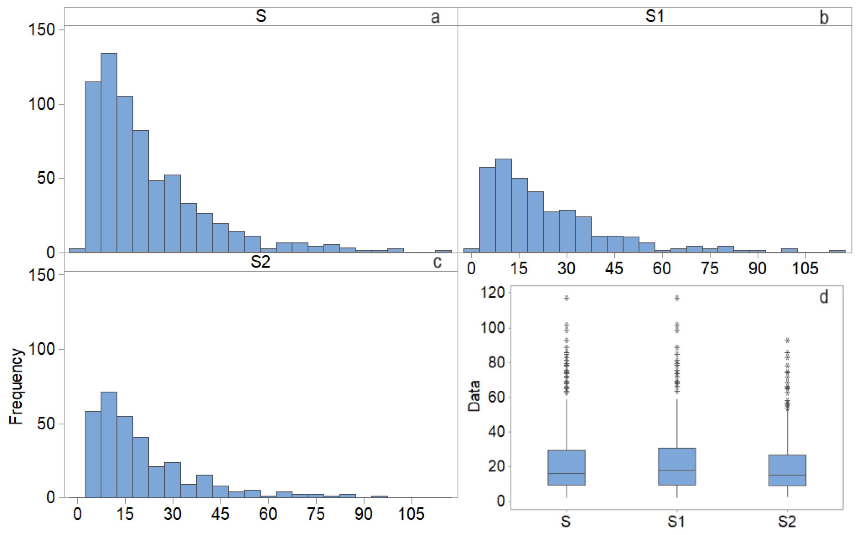
Figure 4.
The study’s flowchart.
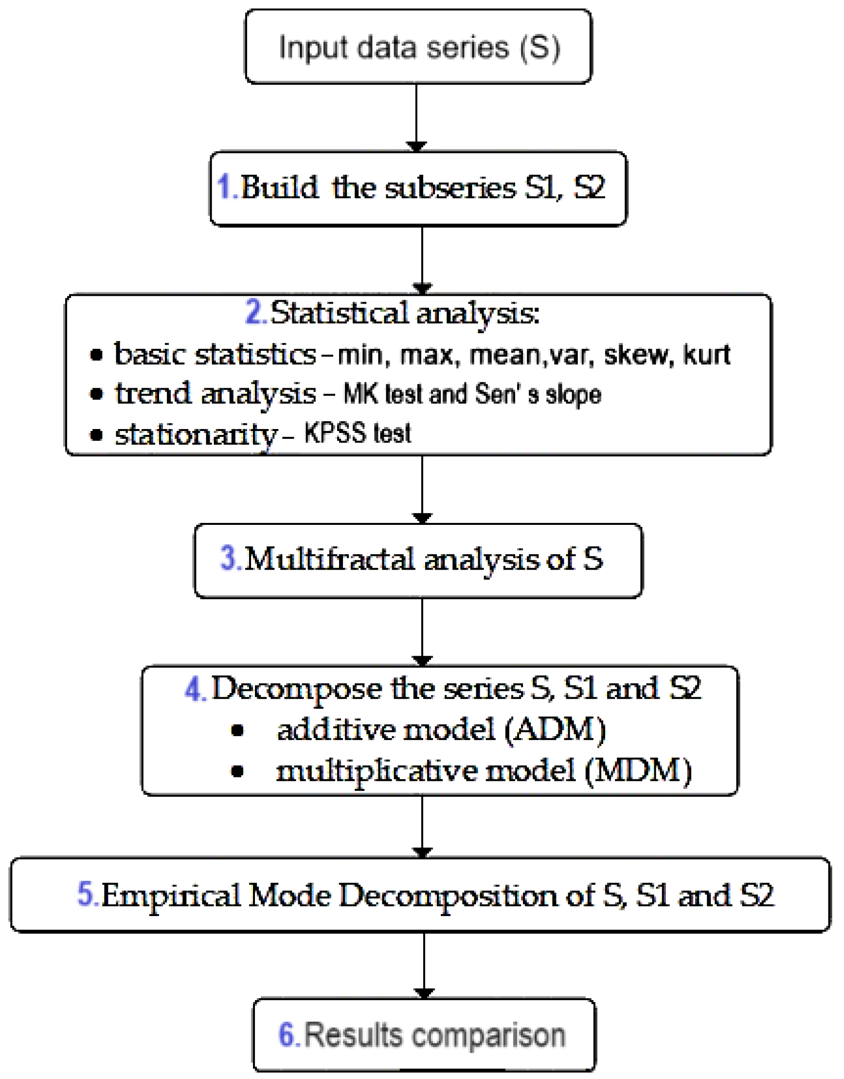
Figure 5.
Results of the multifractal analysis: (a) the mass exponent; (b) the chart of the generalized Hurst exponent; (c) the segmentation function; (d) the f(α) spectrum.
Figure 5.
Results of the multifractal analysis: (a) the mass exponent; (b) the chart of the generalized Hurst exponent; (c) the segmentation function; (d) the f(α) spectrum.
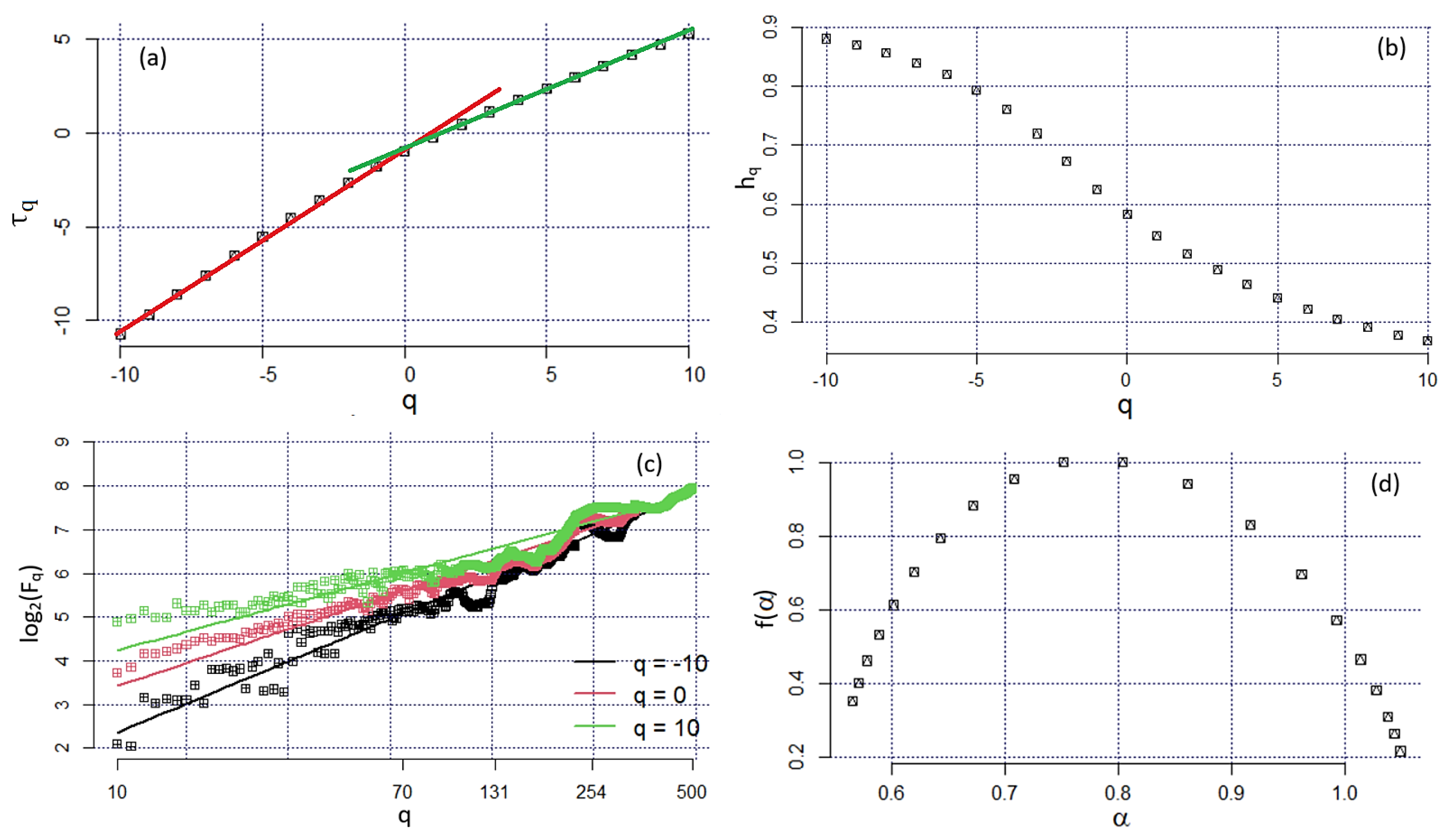
Figure 6.
The ADM for S: (a) the initial series (series), (b) the trend obtained by the moving average of the 12-th order, (c) the seasonality indices, and (d) the residual.
Figure 6.
The ADM for S: (a) the initial series (series), (b) the trend obtained by the moving average of the 12-th order, (c) the seasonality indices, and (d) the residual.
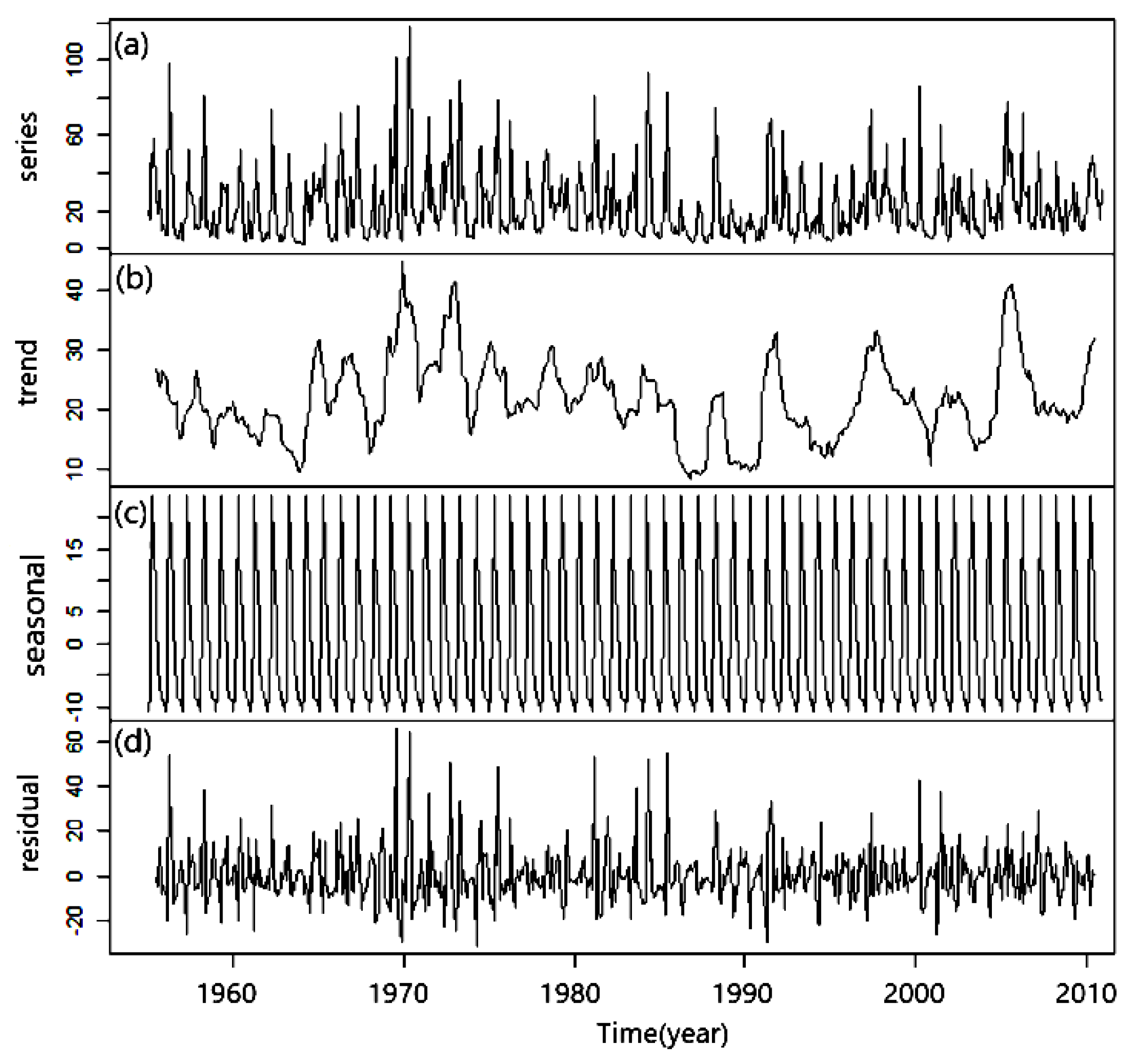
Figure 7.
The MDM for S: (a) the initial series (series), (b) the trend obtained by the moving average of the 12-th order, (c) the seasonality indices, and (d) the residual.
Figure 7.
The MDM for S: (a) the initial series (series), (b) the trend obtained by the moving average of the 12-th order, (c) the seasonality indices, and (d) the residual.
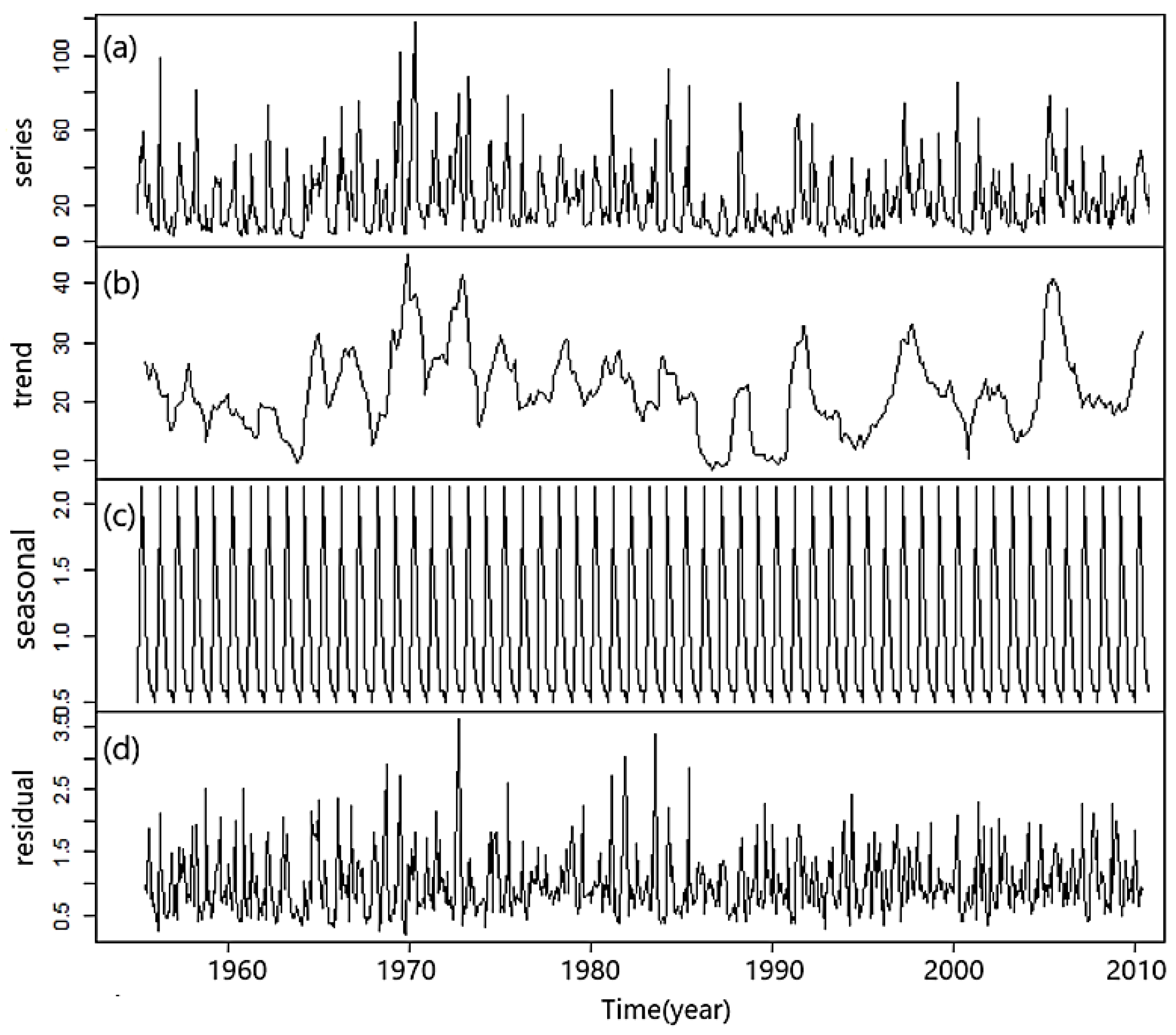
Figure 8.
(a) The residual correlogram in the ADM, (b) the residual histogram in the ADM, (c) the residual correlogram in the MDM, and (d) the residual histogram in the MDM.
Figure 8.
(a) The residual correlogram in the ADM, (b) the residual histogram in the ADM, (c) the residual correlogram in the MDM, and (d) the residual histogram in the MDM.
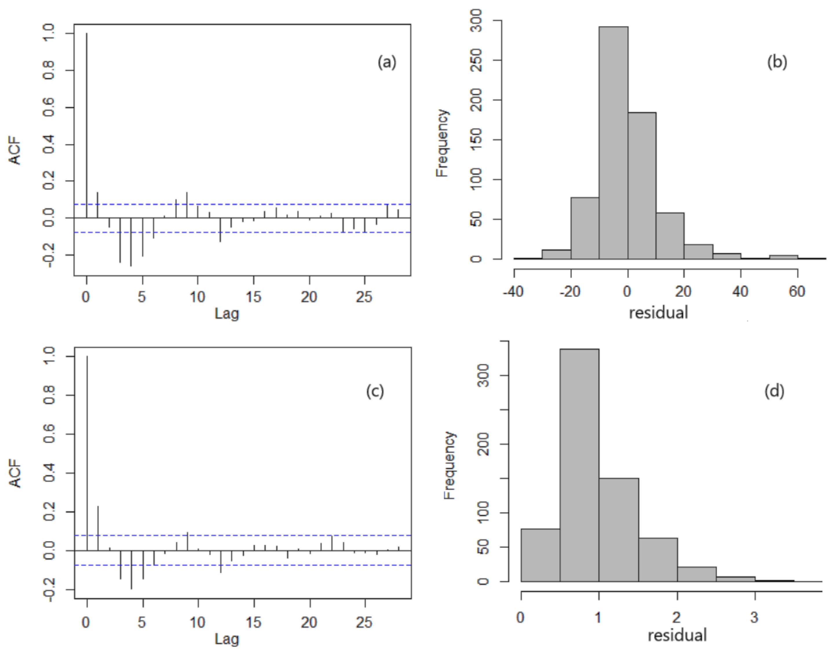
Figure 9.
Details for building IMFs with spline interpolation for IMF 3 (left) and by fine tuning for IMF 4 (right) of the monthly series.
Figure 9.
Details for building IMFs with spline interpolation for IMF 3 (left) and by fine tuning for IMF 4 (right) of the monthly series.
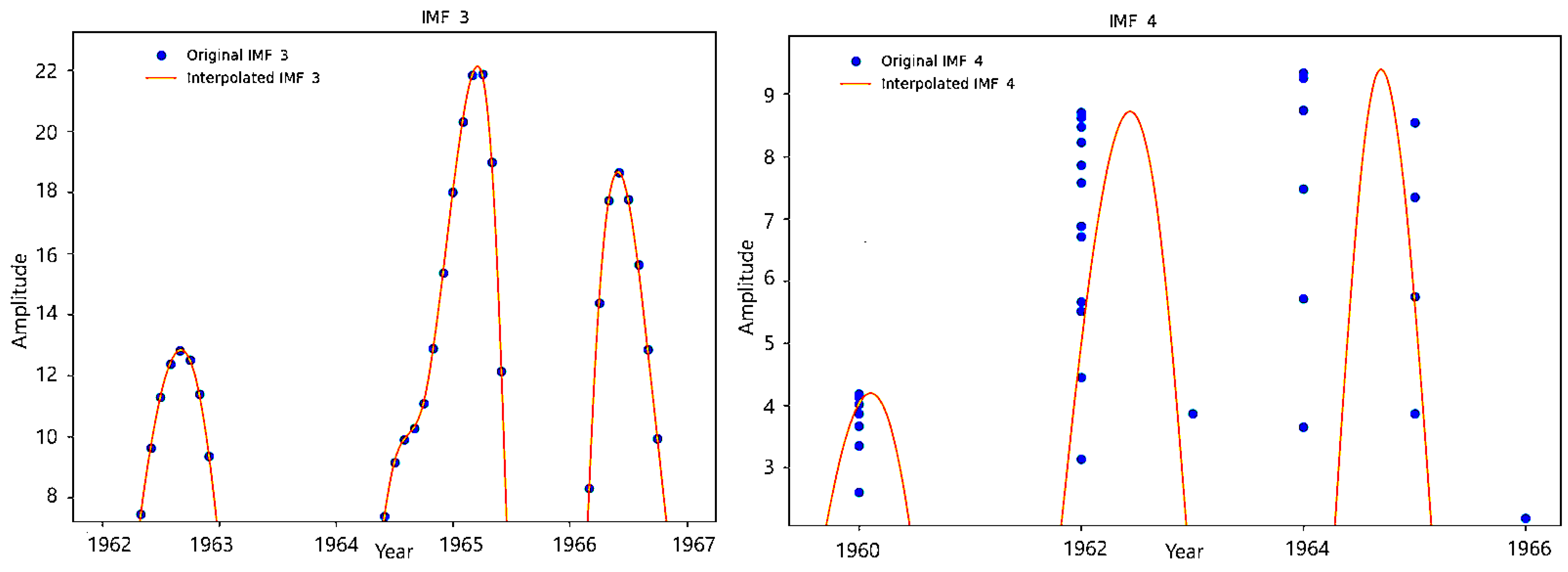
Figure 10.
EMD of the S series: IMF 1, IMF8, and the residuals.
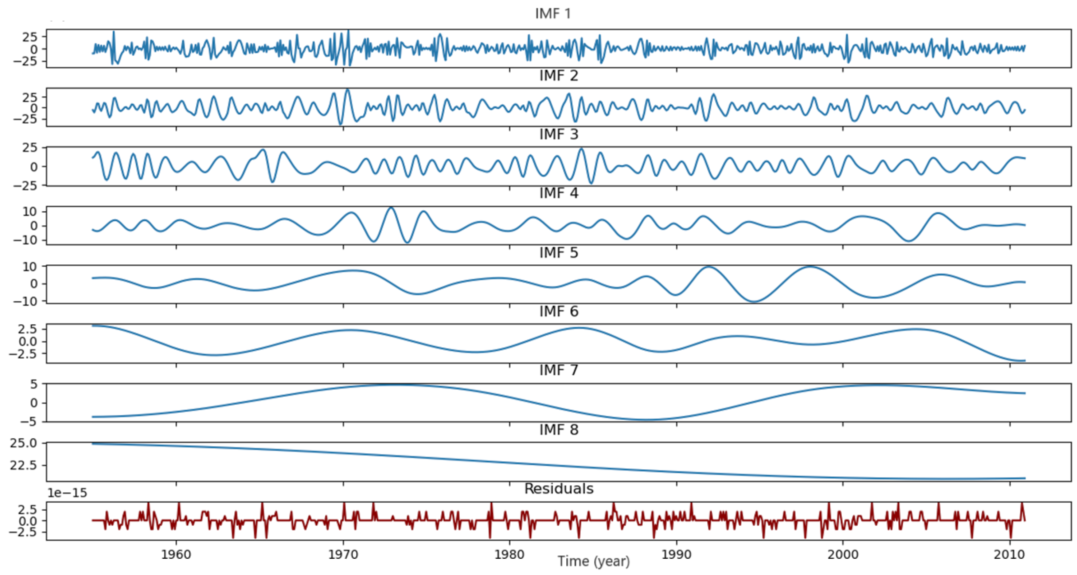
Figure 11.
S1 (left) and S2 (right) series.

Figure 12.
(a) IMF1 for S1, (b) IMF1 for S2, (c) IMF2 for S1, (d) IMF2 for S2, (e) IMF 3 for S1, (f) IMF 3 for S2, (g) IMF 4 for S1, (h) IMF 4 for S2, (i) IMF5 for S1, (j) IMF5 for S2, (k) IMF6 for S1, (l) IMF6 for S2, (m) residual for S1, and (n) residual for S2.
Figure 12.
(a) IMF1 for S1, (b) IMF1 for S2, (c) IMF2 for S1, (d) IMF2 for S2, (e) IMF 3 for S1, (f) IMF 3 for S2, (g) IMF 4 for S1, (h) IMF 4 for S2, (i) IMF5 for S1, (j) IMF5 for S2, (k) IMF6 for S1, (l) IMF6 for S2, (m) residual for S1, and (n) residual for S2.

Table 1.
The p-values in the MK, SMK, and KPSS test, and Sen’s slopes (marked with * inside the brackets).
Table 1.
The p-values in the MK, SMK, and KPSS test, and Sen’s slopes (marked with * inside the brackets).
| Series | MK | SMK | KPSS Trend | KPSS Level |
|---|---|---|---|---|
| S | 0.2851 | 0.2850 | 0.0571 | 0.1000 |
| S1 | 0.0290 (0.0139 *) | 0.0289 (0.0139 *) | 0.0891 | 0.1000 |
| S2 | 0.0000 (0.0311 *) | 0.0000 (0.0311 *) | 0.1000 | 0.6550 |
Table 2.
Seasonality indices in the ADM and MDM for the S series.
| Index | January | February | March | April | May | June | July | August | September | October | November | December |
|---|---|---|---|---|---|---|---|---|---|---|---|---|
| ADM | −10.7800 | −8.3037 | 3.4178 | 23.5093 | 15.5835 | 7.7747 | 4.6647 | −3.2790 | −6.2985 | −8.6096 | −8.8271 | −8.8521 |
| MDM | 0.4986 | 0.6410 | 1.2014 | 2.1329 | 1.6923 | 1.3937 | 1.1742 | 0.834 | 0.6874 | 0.5811 | 0.5816 | 0.5820 |
Table 3.
Seasonality indices in the MDM for S1 and S2.
| Series | January | February | March | April | May | June | July | August | September | October | November | December |
|---|---|---|---|---|---|---|---|---|---|---|---|---|
| S1 | 0.4751 | 0.6289 | 1.1361 | 2.1553 | 1.7975 | 1.3180 | 1.2582 | 0.8205 | 0.6734 | 0.5467 | 0.5985 | 0.5918 |
| S2 | 0.5380 | 0.6739 | 1.3000 | 2.1215 | 1.5102 | 1.4778 | 1.0937 | 0.7758 | 0.7134 | 0.6280 | 0.5785 | 0.5893 |
Disclaimer/Publisher’s Note: The statements, opinions and data contained in all publications are solely those of the individual author(s) and contributor(s) and not of MDPI and/or the editor(s). MDPI and/or the editor(s) disclaim responsibility for any injury to people or property resulting from any ideas, methods, instructions or products referred to in the content. |
© 2024 by the authors. Licensee MDPI, Basel, Switzerland. This article is an open access article distributed under the terms and conditions of the Creative Commons Attribution (CC BY) license (https://creativecommons.org/licenses/by/4.0/).
Share and Cite
MDPI and ACS Style
Bărbulescu, A.; Mohammed, N. Study of the River Discharge Alteration. Water 2024, 16, 808. https://doi.org/10.3390/w16060808
AMA Style
Bărbulescu A, Mohammed N. Study of the River Discharge Alteration. Water. 2024; 16(6):808. https://doi.org/10.3390/w16060808
Chicago/Turabian StyleBărbulescu, Alina, and Nayeemuddin Mohammed. 2024. "Study of the River Discharge Alteration" Water 16, no. 6: 808. https://doi.org/10.3390/w16060808
Note that from the first issue of 2016, this journal uses article numbers instead of page numbers. See further details here.