Abstract
In the context of accelerating urbanisation, the issue of urban stormwater flooding security has garnered increasing attention. Further development of urban stormwater management techniques is imperative to achieve more stable, precise, and expeditious simulation outcomes. The calibration of model parameters, which is a pivotal phase in stormwater simulation endeavours, is hampered by challenges such as substantial subjectivity, time intensiveness, and low efficiency. Therefore, this study introduces a parameter calibration model coupled with the Non-dominated Sorting Genetic Algorithm III (NSGA-III). This model utilises the Nash–Sutcliffe efficiency (NSE) and peak relative error (PE) values for various rainfall events as objective functions to calibrate and assess the study target. The two rainfalls used for rate determination had NSE values greater than 0.9 and absolute PE values less than 0.17; the rainfall used for validation had NSE values greater than 0.9 and absolute PE values less than 0.27. Thus, the results of the model for the rate determination of the parameters are reliable. In addition, the inverted generation distance and hypervolume values indicate that the iterative process of the algorithm during population evolution demonstrated stable iterative outcomes and ensured sound population quality. Both reach relative stability after 40 iterations. In conclusion, the proposed multi-objective parameter calibration model integrated with NSGA-III offers dependable calibration results and robust computational efficacy, presenting novel avenues and perspectives for urban stormwater model parameter calibration and simulation.
1. Introduction
With the acceleration of social progress and urbanisation, the gradual expansion of urban areas has made urban flood safety issues more important [1]. Flood safety issues, including efficient and stable urban inundation warning systems and the utilisation of stormwater technologies for urban water resource management, rely heavily on stable, accurate, and rapid model simulation techniques [2]. Numerical models of urban hydrodynamic processes are crucial non-engineering measures for flood prevention. They provide vital technological support for urban stormwater disaster prevention and reduction, making them a focal point for research in related domains.
The Storm Water Management Model (SWMM) is a classic hydrodynamic model [3] that employs nonlinear reservoir-based methods for determining surface runoff and constant flow, kinematic waves, or dynamic wave algorithms for pipe network routing [4]. It was developed by the United States Environmental Protection Agency in 1971 and has undergone over 50 years of iterative updates, encompassing five major iterations. SWMM operates through interconnected computational and service modules [5]. The computational simplicity and open-source nature of this model [6] have led to its widespread adoption. Its scope includes single and continuous rainfall events, conveyance processes within a pipe network, and pollutant accumulation and transport processes [7]. Additionally, the simulation process offers visualisation capabilities. The computational modules include runoff, conveyance, expanded conveyance, and storage/treatment, whereas the service modules include plotting, statistics, coupling, and rainfall.
During the modelling process, the input data for the SWMM can be categorised into hydrological and hydraulic parameters [8]. Some of these parameters can be obtained based on their physical significance using relevant technical means, whereas others involve uncertain parameters that are initially obtained through empirical approaches and subsequently refined through calibration and validation. Due to the excellent computational performance of the SWMM (5.2.1) and the fact that it is free and open-source software, which allows for easy secondary development, it is possible to consider the development of a SWMM for automated parameter rates. In 2020, the Open Water Analytics organisation developed the PySWMM (1.5.1) third-party package by merging the SWMM interface with Python and the SWMM application [9]. This package makes direct use of the SWMM’s computational engine and facilitates data interaction. Although the PySWMM code itself does not contain a parameter optimisation module, coupling the optimisation algorithms with the model enables automatic parameter optimisation and calibration.
Model calibration primarily involves manual and automatic methods [10]. Manual calibration entails the iterative adjustment of model parameters through trial and error to determine the optimal parameter combination, making it a monotonous and intricate process that requires iterative analysis by modellers and relies heavily on their practical experience [11]. The modelling results are susceptible to significant artificial influences. With advances in computer technology, researchers have progressively replaced manual parameter tuning with various optimisation algorithms [12] to facilitate automatic parameter calibration.
Optimisation algorithms can be categorised into deterministic and heuristic optimisation algorithms. Traditional optimisation algorithms, such as the complex urban stormwater model simulations, are subject to computational burdens that make their practical application challenging. In the early 1980s, heuristic optimisation algorithms introduced new avenues for hydrodynamic model calibration [13]. Heuristic algorithms emulate the process of biological organisms dealing with complex problems, using computational techniques to achieve the automatic optimisation of model parameters. This approach significantly reduces the human influence and time consumption associated with manual calibration, thereby enhancing modelling efficiency and credibility. Kim et al. established a coupled SWMM underground drainage network multi-objective automatic parameter calibration model for Seoul [14] using a Non-dominated Sorting Harmony Search (NSHS) algorithm. Experimental testing revealed that the calibrated model framework could effectively reflect system characteristics and address issues in pipe design, planning, and management, thereby contributing to simulation research. Ref. [15] employed a combination of particle swarm optimisation (PSO) and Sequential Quadratic Programming (SQP) for SWMM model parameter calibration, providing a scientifically effective approach with strong local search capabilities. Behrouz et al. [16] integrated the ostrich algorithm with the SWMM to develop an open-source calibration tool called OSTRICH-SWMM, which offers various optimisation algorithms for single-objective or multi-objective automatic calibration, thereby offering new tools for automatic SWMM calibration. In addition to optimising the model calibration process, optimisation algorithms are frequently used to couple hydrological models [17] and compare various development schemes and hydraulic structure layout scenarios. The algorithmic selection of models allows for a comprehensive consideration of ecological and environmental benefits, as well as cost conditions, significantly enhancing urban water management capabilities and efficiency. For example, Li et al. [18] employed a generalised diversion method to combine the flow transmission chain in the runoff part of the SWMM to simulate LID layout scenarios. By comparing the performance of different scenarios, the optimal solution can be selected, leading to greater environmental benefits than those of similar models.
The Genetic Algorithm (GA) is an evolutionary algorithm that simulates natural genetic mechanisms and biological evolution theory to search for optimal solutions. It was first proposed by John Holland in 1975 [19]. The GA encodes feasible solutions assumed for specific problems in data structures that are similar to chromosomes. Each chromosome represents a solution vector, and a collection of solution vectors forms a solution vector population. The GA’s key steps include solution vector encoding, population of solution vectors, fitness function evaluation, genetic operator selection, crossover, and mutation [20], with each solution corresponding to an individual in a biological population. Owing to its global search capability, the GA has extensive applications [21] and is commonly used in practical problems such as automatic control, computer science, and fault diagnosis. It is suitable for solving complex nonlinear and multidimensional optimisation problems. In 1995, Liong et al. [22] first applied a GA to calibrate the SWMM. They aimed to minimise the peak flow as the objective function and calibrated eight parameters in a subcatchment of a Singapore watershed. This study employed three rainfall events for calibration and verification to demonstrate the applicability of the GA in hydrological model calibration.
However, as the computational complexity of these models increased, traditional GAs began to exhibit limitations and shortcomings. Several improved algorithms have recently been proposed. Non-dominated Sorting GA III (NSGA-III) builds upon conventional GAs by incorporating an elitist strategy [23]. This involves a hierarchical process carried out before the selection operation, along with the introduction of widely distributed reference points to maintain population diversity.
In this study, the parameters and their value ranges were first determined based on the practical experience of the researchers, the SWMM manual, and references from the literature. Subsequently, the NSGA-III algorithm was used for multi-objective parameter calibration. Since the NSGA-III algorithm can be used to solve multi-objective problems in three dimensions and above, the researchers endeavoured to use both Nash–Sutcliffe efficiency (NSE) and peak relative error (PE) as the objective functions. This was performed to increase the peak accuracy of the simulation results while ensuring the overall correctness of the simulation results. It can also speed up the model-solving process. Meanwhile, the researchers innovatively used a set of parameters to rate multiple rainfalls simultaneously, allowing the evaluation of the simulation accuracy of the same set of parameters for different rainfalls and further improving the accuracy of the parameter rate results. In this paper, the researchers selected three real rainfall events and applied the model to an independent sub-basin stormwater drainage network system in a city to establish a four-dimensional target calibration model. This study aims to provide new insights into urban stormwater modelling in the context of smart water management and to improve the predictive performance of the SWMM model, providing technical support for the automatic calibration of SWMM model parameters and the accurate simulation and application of this model.
2. Methodology
2.1. NSGA-III
Deb proposed a novel multi-objective evolution algorithm, NSGA-III, in 2014 [24]. Its fundamental framework is similar to that of the traditional NSGA-II, involving crossover and mutation to generate new individuals and employing a fast non-dominated sorting method to partition old and new individuals. However, the selection mechanisms were different. NSGA-II ranks [25] individuals based on their crowding distances, which may lead to an uneven distribution of individuals in the objective space and hinder the discovery of globally optimal solutions. The NSGA-III selection operator comprises two steps [26]: first, non-dominated solutions are divided into layers; second, individuals from the last non-dominated layer are selected to enter the next generation. The overall framework of the algorithm is described as follows:
- (1)
- Population initialisation: Generate the initial population, and set the number of evolutionary generations to one.
- (2)
- Judge whether the first-generation sub-population has been generated: If so, update the evolutionary generation so that it increases by one. If not, initiate the selection, crossover, and mutation of the initial population to generate the first generation of sub-populations. Meanwhile, update the evolutionary generation such that it increases by one.
- (3)
- Merge the parent population and sub-population into a new population;
- (4)
- Determine whether a new parent population has been generated: If so, calculate the objective function of individuals in the new population and perform non-dominated sorting, selection, crossover, and mutation. Otherwise, perform selection, crossover, and mutation operations on the generated parent population to generate the sub-population.
- (5)
- Termination Criteria: If the iteration limit has been reached, the algorithm terminates; otherwise, the number of evolutionary generations is increased together with a return to step 3.
- (6)
- Output the set of high-quality solutions in the Pareto front.
The NSGA-III selection mechanism enhances computational efficiency, especially for problems with three or more objectives. It builds on NSGA-II to provide improved performance [27]. By introducing a reference point mechanism, NSGA-III enhances the convergence and diversity of a population. It guides search directions, accommodates various forms of objective functions, and addresses complex and diverse multi-objective optimisation problems [28]. The specifics of the reference point mechanism are given below.
- (1)
- Normalising the objective function:
Firstly, M is specified as the number of optimisation objectives, and the minimum value of each objective dimension of the current population zjmin, j ∈ {1, 2, …, M}, is calculated as the ideal point of the current population.
The target value fj(x) for all individuals in each dimension is obtained by subtracting the ideal point in the corresponding dimension:
fj′(x) = fj(x) − zjmin
Calculate the additional target vector zi,max according to the following equation:
ASF(x,w) = maxi = 1M fj′(x)/wi
zi,max = x; argmin ASF(x,wi), wi = (τ, …, τ), τ = 10−6, wij = 1
The intercept of the hyperplane with each target dimension formed by M additional target vectors is aj, j = 1, 2, …, M. If it is not possible to form the hyperplane or the intercept of the hyperplane with each target dimension is not available, let aj be the maximum value of each target dimension.
The normalised objective function value is as follows:
fjn (x) = fj′(x)/(aj − zjmin)
- (2)
- Linking individuals to reference points. Calculate the distance from each individual to all reference lines; the point corresponding to the reference line closest to an individual is the reference point for that individual.
- (3)
- Perform individual selection based on the reference.
2.2. Optimization Model
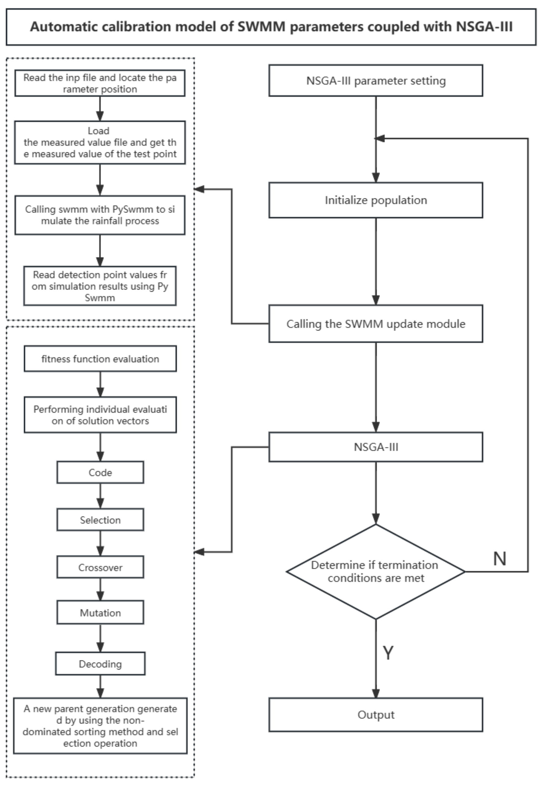
In order to achieve the function of high-dimensional multi-target automatic rate calibration, the researchers coupled the SWMM model with NSGA-III, forming a new model, and the new SWMM automatic parameter calibration model consists of three modules: SWMM parameter extraction and updating, SWMM simulation calculation, and NSGA-III parameter optimisation. The researchers selected eight sensitive parameters for rate determination based on the SWMM manual, the literature, and practical work experience. Two parameters, NSE and PE, were selected as the judgement indicators of model accuracy, and the four indicator data of the two rainfalls were set as the objective function values of NSGA-III, with the same weights of the four values. The model automatic rate calibration workflow is as follows:
- (1)
- Designate two rainfalls as input files for two SWMM projects, respectively, and set the same initial values for both input files.
- (2)
- Set the parameters required by the NSGA-III algorithm.
- (3)
- Generate the initial population for the optimisation algorithm.
- (4)
- Call the SWMM model using PySWMM and custom functions to couple them with SWMM and perform model simulation, including (a) reading the project input file and locating the parameters that need to be modified; (b) reading the measured values of the test points; (c) mobilising the model and performing rainfall runoff simulations using PySWMM; and (d) reading the simulated values of the model of the test points.
- (5)
- Calculate the simulated and measured values based on the objective function.
- (6)
- Continue the algorithmic process of selection, crossover, and mutation from the NSGA-III algorithm.
- (7)
- Determine whether the termination conditions have been met.
- (8)
- Output the results, including the success of rate determination, the number of iterations, the optimal solution, and the evaluation of the quality of the population.
A detailed workflow of the algorithm is shown in Figure 1.

Figure 1.
Flowchart of the multi-objective automatic calibration process for urban stormwater model coupled with NSGA-III.
3. Case Study
3.1. Study Area
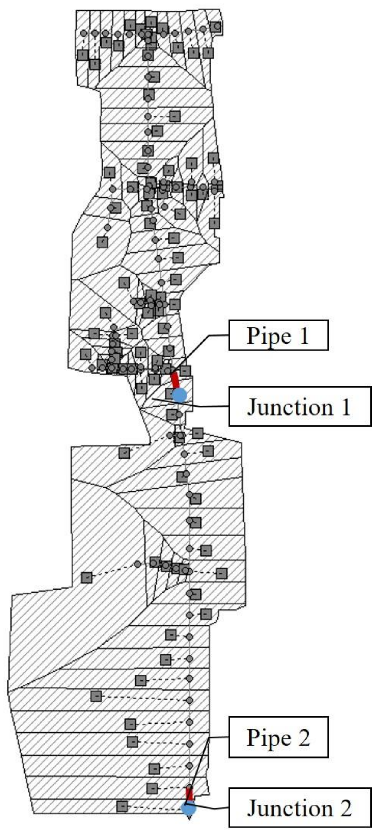
The research data used in this study were based on a small study area. According to blueprints, the study area covers approximately 1.5 km2. The drainage network comprised 98 nodes, 98 pipe segments, 98 subcatchments, and one outlet, with a total pipe length of approximately 4.8 km. The study area comprises 32.5% residential areas, 35.2% impervious surfaces, 14.2% roads, 7.7% vegetation, and 10.4% bare soil (Figure 2). Flow-monitoring data from nodes 1 and 2, as well as pipes 1 and 2, were used as foundation data for rainfall and runoff analysis, with a sampling interval of 5 min.

Figure 2.
Diagram of the SWMM modelling results.
The detection data for this experiment mainly came from the field detection statistics of the experimental stations deployed in the study area, which were mainly measured via rain gauges and flow meters, with a high degree of confidence in the data and a sampling period of 5 min. During the data collection process, the researchers double-checked the data to ensure their accuracy.
The overall topography of the study area is relatively gentle, and it is high in the north and low in the south, with a maximum height difference of about 8.2 m. The overall topographic trend of the study area and the pipeline drainage direction coincide. This study’s values for the width of partial catchments were calculated using formulas based on the definition provided in the SWMM manual and findings from other researchers’ studies.
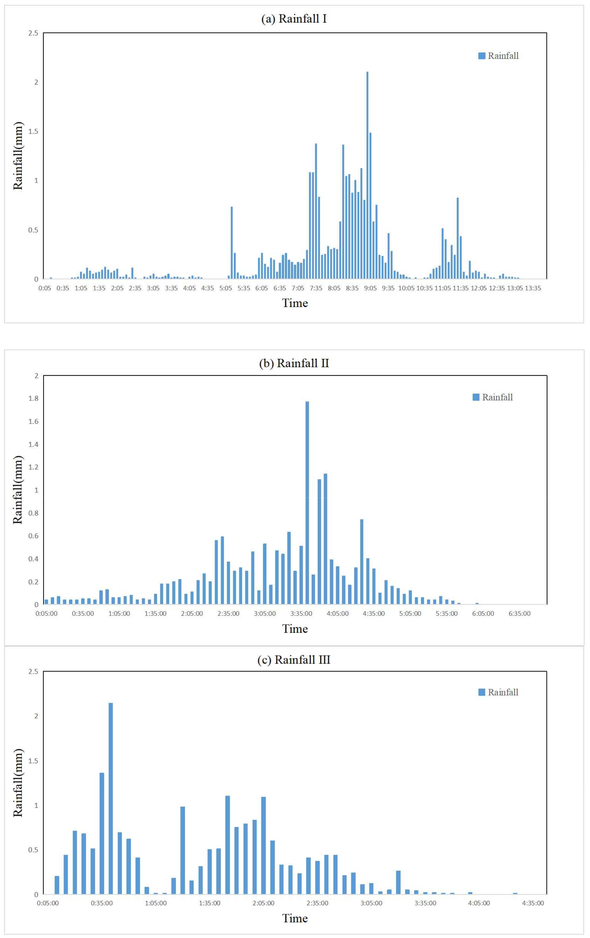
Three rainfall data (Figure 3a–c) sets were selected for this study: two for rate determination and one for calibration. Long Rainfall I and short Rainfall II were selected to improve the adaptability of the model rate determination results, and bimodal Rainfall III, which was not involved in rate determination, was selected to validate the usability of the model.
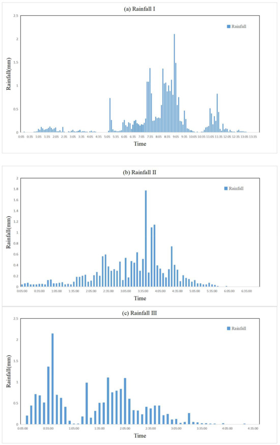
Figure 3.
Typical rainfall: (a) Rainfall I; (b) Rainfall II; and (c) Rainfall III.
3.2. Objective Functions
3.2.1. NSE Coefficient
The NSE coefficient is a standardised statistical metric. An NSE value approaching 1 indicates a stronger correlation between the observed and predicted data. When the NSE value falls within the range of 0–1, it signifies an acceptable goodness of fit for the calibration results of the model.
3.2.2. PE
The NSE coefficient has high confidence in determining the overall fit of the rainfall calendar; however, its confidence in determining the fit of specific peaks in the overall process is average. Therefore, this study introduces the PE value to analyse the fit for the peaks of the nodes and pipes.
PE represents the error between the observed peak runoff and the predicted peak runoff.
The variables used in the formula above are explained below:
I—the time step; N—total time step of the input data;—observed value at time step i;—simulated value at time step i;—observed average value;—simulated peak flow;—observed peak flow.
3.3. Optimal Variables
According to the computational principles of the SWMM, the selected parameters can be categorised into permeable and impermeable zones, which leads to the problem where a large number of possibilities can arise from combinations of parameters in both permeable and impermeable zone groups. This was addressed in this study by selecting two rainfall events of different calendar times and intensities for rate determination, and one rainfall event was used for validation to corroborate the usability of the model rate determination results for the study area model.
Based on the previous literature [29,30,31] and the recommendations of the SWMM model manual, together with the practical experience of the researchers in regard to the modelling process, eight relatively sensitive hydrological parameters were selected for further study, and the specific ranges of values for each parameter are listed in Table 1.

Table 1.
Model parameter values.
4. Results and Discussion
4.1. Evaluation of Parameter Calibration Results
By setting the iteration count to 100 generations, a GA was employed to optimise the eight parameters of the SWMM. The optimal parameter sets are presented in Table 2.
Table 2.
Model parameter calibration results.
The optimal parameter set from Table 3 was applied to the SWMM. For the three rainfall events in the experiment, the corresponding node water levels and flow process data were simulated and compared with observed values. The results are presented in Table 3 and Figure 4, Figure 5 and Figure 6.
Table 3.
Model calibration evaluation metrics.
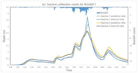
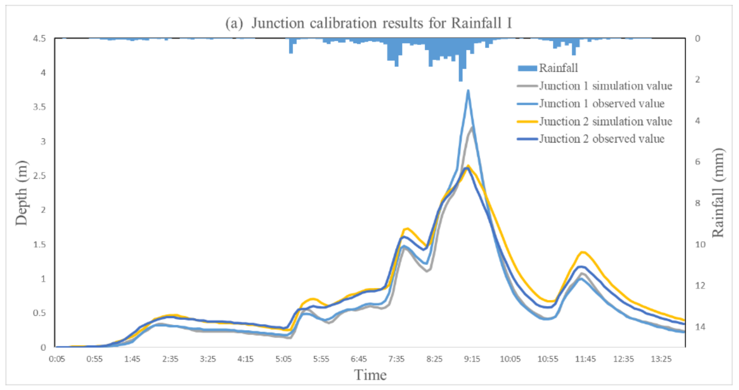
Figure 4.
Calibration results for Rainfall I: (a) junction and (b) pipe.
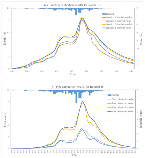
Figure 5.
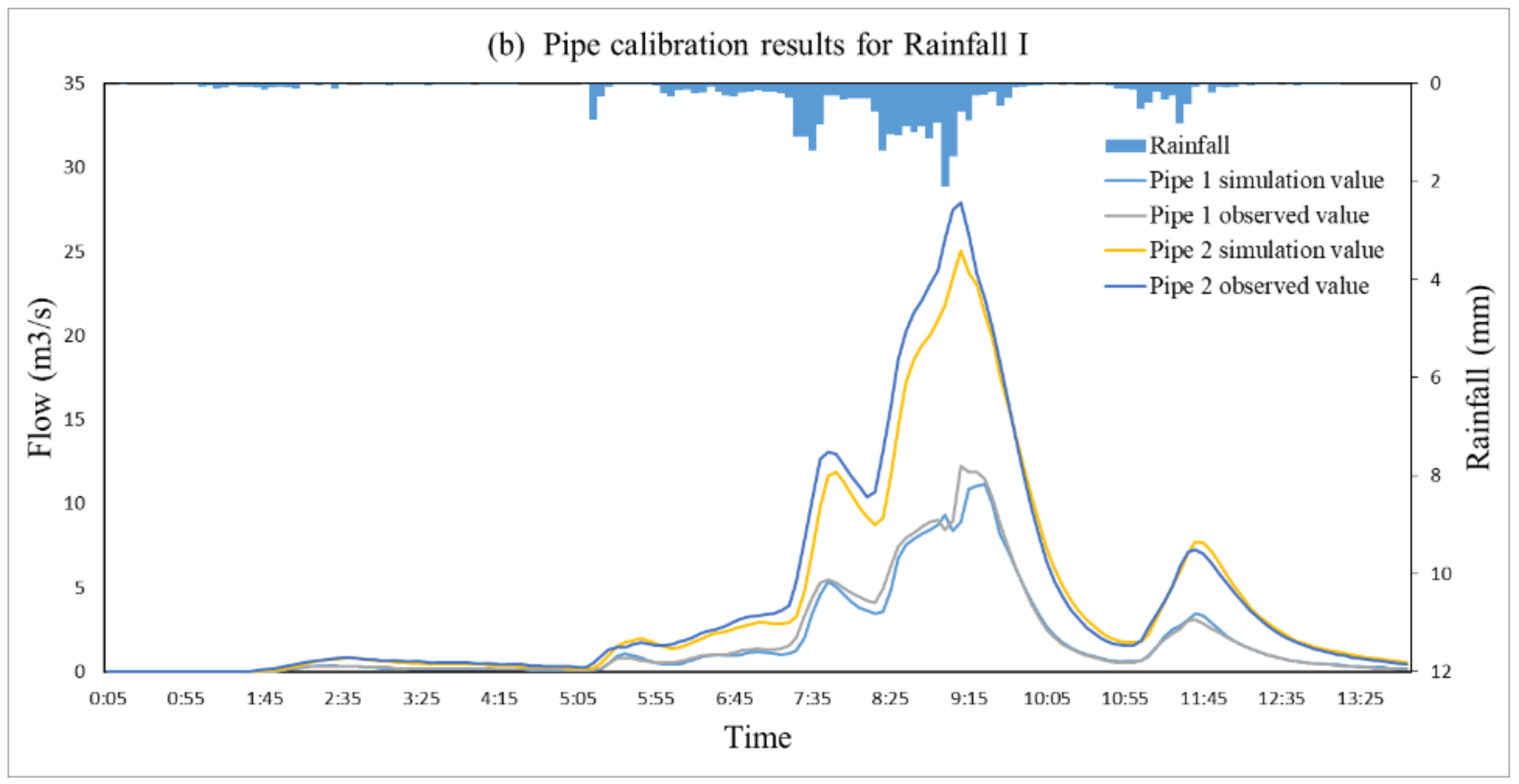
Calibration results for Rainfall II: (a) junction and (b) pipe.

Figure 6.
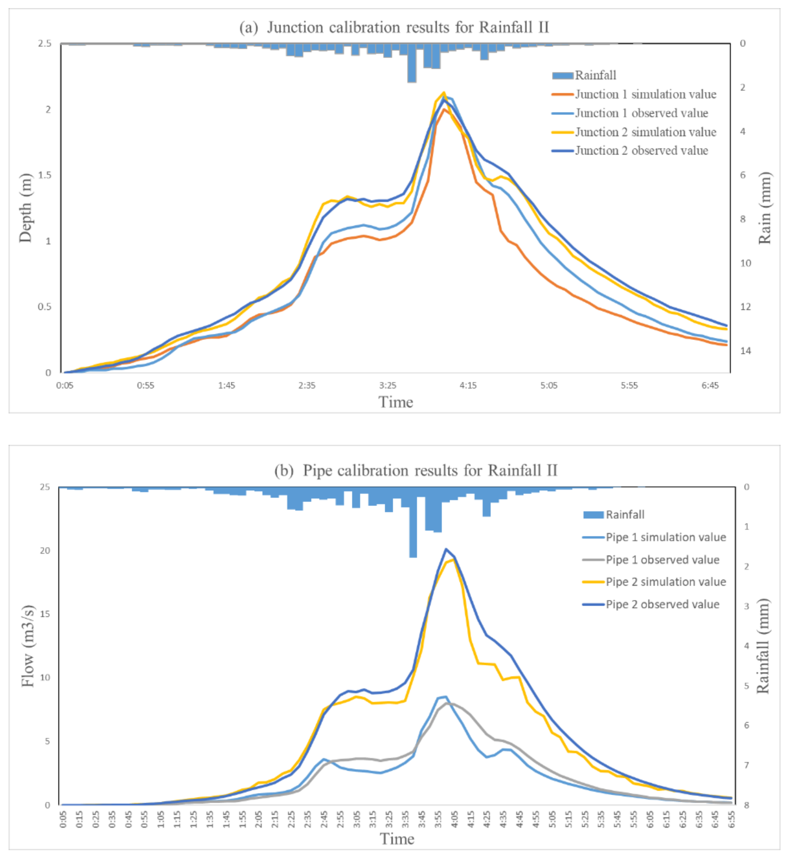
Calibration results for Rainfall III: (a) junction and (b) pipe.
Figure 4a,b depict the simulation results of Rainfall Event I and the numerical comparisons between the simulated and observed values of the nodes and pipes. For instance, for Node 1, the observed peak water level during rainfall was 3.74 m, observed at 9:10, while the simulated peak was 3.2 m, observed at 9:15. Similarly, Node 2 had an observed peak of 2.61 m at 9:05, and the simulated peak was 2.65 m at 9:10. Pipe 1 had an observed peak flow rate of 12.25 m3/s at 9:10, and the simulated peak was 11.2 m3/s at 9:25. Pipe 2 exhibited a peak flow rate of 27.9 m3/s at 9:10, and the simulated peak was 25.6 m3/s at 9:10. The peak values and occurrence times of the measurement points align well with the rainfall process, and the evaluation metrics between the observed and simulated values indicate favourable agreement, confirming the reliability of the simulation results.
Figure 5a,b present the simulation results of Rainfall Event II and the numerical comparisons between the simulated and observed values of the nodes and pipes. For Node 1, the observed peak water level during rainfall was 2.1 m, observed at 4:00, while the simulated peak was 2 m, occurring at the same time. Similarly, Node 2 had an observed peak of 2.07 m at 4:00, and the simulated peak was 2.03 m at the same time. Pipe 1 had an observed peak flow rate of 7.99 m3/s at 4:00, and the simulated peak was 8.51 m3/s at the same time. Pipe 2 had an observed peak flow rate of 20.11 m3/s at 4:00, and the simulated peak was 19.32 m3/s at 4:05. The peak values and occurrence times of the measurement points aligned well with the rainfall process, and the evaluation metrics between the observed and simulated values indicated favourable agreement, reaffirming the reliability of the simulation results.
Figure 6a,b present the simulation results of Rainfall Event III and numerical comparisons between the simulated and observed values of the nodes and pipes. Rainfall Event III served as the validation scenario for this experiment. The results indicate that for Node 1, the observed peak water level during rainfall was 2.15 m, occurring at 2:10, while the simulated peak was 2.06 m at 2:01. Similarly, Node 2 had an observed peak of 2.1 m at 2:10, and the simulated peak was 2.21 m at the same time. Pipe 1 had a ratio of 8.15 m3/s at 2:10, and the simulated peak was 7.9 m3/s at the same time. Pipe 2 had an observed peak flow rate of 20.48 m3/s at 2:10, and the simulated peak was 18.42 m3/s at the same time. The peak values and occurrence times of the measurement points aligned well with the rainfall process, and the evaluation metrics between the observed and simulated values indicated favourable agreement, reinforcing the reliability of the simulation results.
In summary, the results predicted for the three rainfall events using the parameter set demonstrated good agreement. The observed and simulated values exhibited a high degree of similarity, with consistent overall trends, coincident peak occurrence times, and similar peak flow rates. The NSE values for Rainfall Event I were all greater than 0.98, and the absolute values of PE were all less than 0.2 (Table 3). For Rainfall Event II, the NSE values were all greater than 0.92, with absolute PE values less than 0.2. Similarly, for Rainfall Event III, the NSE values were all greater than 0.92, and the absolute PE values were all less than 0.3. Across all three rainfall events, the NSE values were all above 0.91, and the absolute PE values were less than 0.3.
Overall, the automatic rate model studied in this paper is more accurate and stable due to its new considerations and design for rainfall fields and objective functions. Some scholars based their approach on the BP neural network algorithm for the automatic rate determination of SWMM parameters [32], and the NSE values of their research results are greater than 0.85; in comparison, the NSE values of this paper are greater than 0.91, which is a significant improvement. At the same time, the automatic rate determination of SWMM parameters based on the BP neural network algorithm can only rate one rainfall datum each time, and the use of the rate determination results is more limited. In addition, the automatic rate model using the traditional genetic algorithm (GA) [33] is limited by the dimensionality of the objective function, which makes the accuracy of the rate results unstable, with the NSE value fluctuating between 0.55 and 0.9, compared with the model rate results in this study (NSE > 0.91), which are better.
Therefore, the calibration results of this model were outstanding, with the evaluation metrics consistently surpassing acceptable thresholds. This indicates that the coupled model is stable and reliable.
4.2. Evaluation of Algorithm Results
To assess the inherent solving effectiveness of an algorithm, the academic community has introduced a range of algorithm evaluation metrics that primarily appraise the convergence and distribution characteristics of an algorithm. In this study, the inverted generation distance (IGD) and hypervolume (HV) were employed as evaluation metrics for the coupled algorithm. Both IGD and HV concurrently measure the convergence and distribution properties of an algorithm and are widely applied.
IGD comprehensively evaluates the convergence and diversity of an algorithm by calculating the distances between the objective vectors of each point in the true Pareto optimal solution set and the front of the obtained Pareto optimal solution set. Let P* represent the true Pareto solution set and P denote the obtained Pareto optimal solution set. IGD is defined by the following formula:
where d(v,P) is the minimum Euclidean distance between the solution, y, in P* and the solutions in the population, P, and is the size of the population P*. When the population remains constant, the IGD value is determined by the sum of the minimum Euclidean distances between all solutions in the true Pareto optimal solution set P* and the obtained Pareto optimal solution set P. Only when the obtained solution set demonstrates good convergence and diversity will the IGD value decrease. Hence, the IGD value was employed to measure the overall performance of the algorithm, where a smaller IGD value indicates better overall performance.
HV can simultaneously assess the distribution and convergence of obtained solutions. When calculating HV, a reference point is required, which is generally set as the maximum value for each objective in the true Pareto front. Let R represent the union of the maximum values. Given that PF* represents the solutions obtained by the multi-objective evolutionary algorithm, HV is defined as follows:
where Leb(A) is the Lebesgue measure of set A. A larger HV value indicates better overall performance of the algorithm.
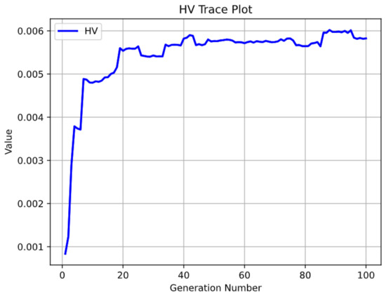
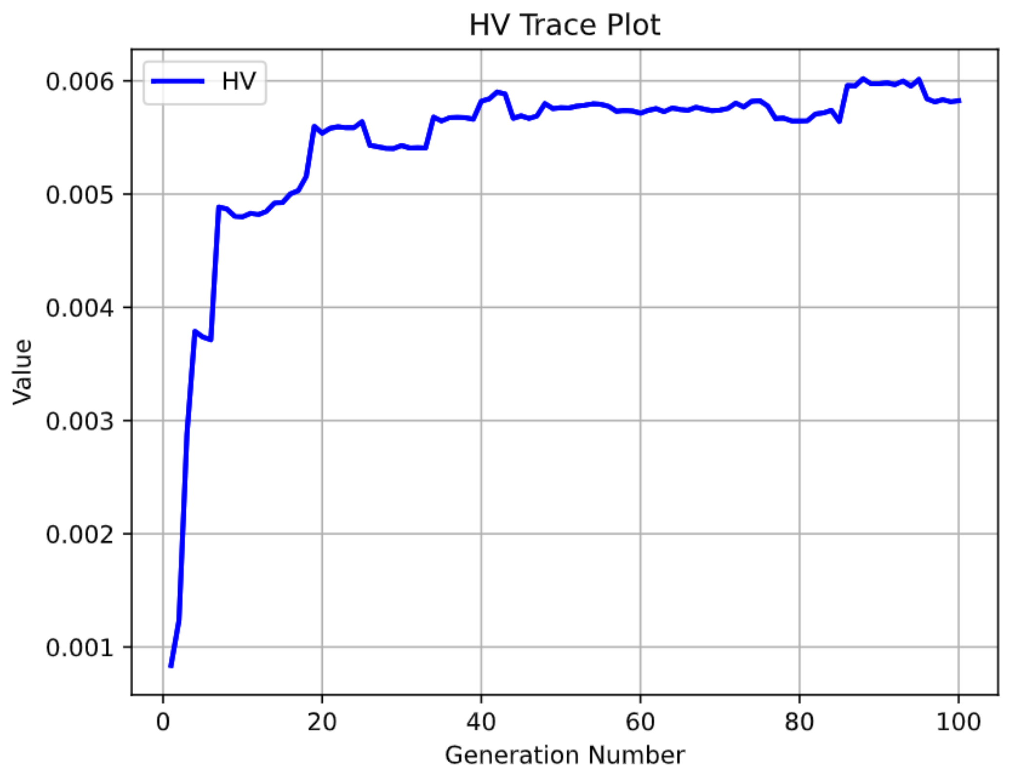
Figure 7.
HV index curve chart.

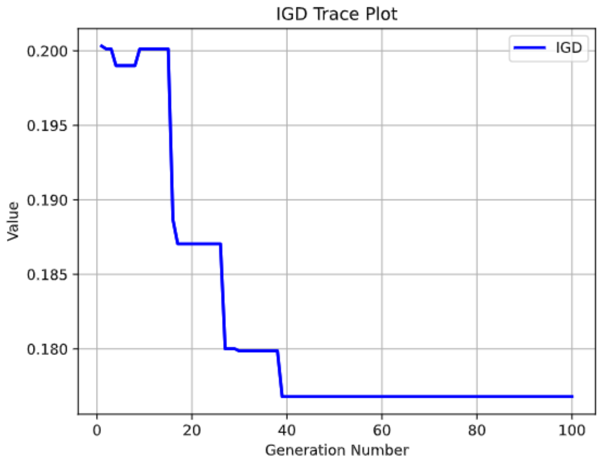
Figure 8.
IGD index curve chart.
Figure 7 shows that the algorithm reaches an HV of 0.006 after 20 iterations and remains stable thereafter. This indicates that the algorithm can produce a better set of solutions for solving the multi-objective optimisation problem, which can cover a large range in the objective function space. After the HV stabilises, further iterations may not significantly change the quality of the solution. Stable HV values indicate that the algorithm has found a set of solutions that are close to the optimal solution, and these solutions can form an equilibrium distribution in the objective function space, which is important for practical decision making and problem solving.
Figure 8 shows that the algorithm reaches an IGD of 0.175 after approximately 40 generations of iterations and remains stable thereafter. IGD is a measure of the distance between the solutions generated by the algorithm and the Pareto front. A smaller IGD value indicates that the algorithm can generate solutions that are closer to the Pareto front, which shows that the algorithm has a better distribution, whereas a stable IGD value proves that the algorithm is robust and reflects whether the distance between the solutions generated by the algorithm and the true front is stable. After reaching a stable IGD value, the distance between the solution generated by the algorithm and the true frontier decreases, and the solution set of the algorithm is already relatively close to the true frontier.
In summary, the algorithm demonstrated good convergence properties after approximately 20 generations and maintained stability thereafter. It can generate a set of solutions that cover a broad range in the objective function space with small distances from the Pareto front, indicating that the algorithm performs well in solving multi-objective optimisation problems.
5. Conclusions
This study employed NSGA-III and PySWMM to research the automatic parameter calibration of the model discussed herein. The calibrated model parameters yielded favourable predictions for the three rainfall events. The similarity between the observed and simulated values was high, exhibiting consistent overall trends, peak timings, and similar peak flow rates. In Rainfall I conditions, the NSE value is greater than 0.98, and the PE absolute value is less than 0.16. In Rainfall II conditions, the NSE values are all greater than 0.92, and the PE absolute values are less than 0.17. In Rainfall III conditions, the NSE value is greater than 0.91, and PE absolute value is less than 0.27. In general, the results of parameter rate determination are considered credible when the NSE value reaches 0.5 or more. In the rate determination results of this model, the NSE values of the three rainfall events are all greater than 0.91, so the fit of the model parameter rate determination is good, and the results of running the model are credible. The algorithm can generate a set of solutions covering a broad range in the objective function space with small distances from the Pareto front, which indicates its strong performance. Overall, the calibration results were great, and the evaluation indicators were reliable, indicating the stability and reliability of the coupled model. The coupled model in this study does not have a specific requirement for the size of the study area, but depending on the modelling process, an area that is too large may require more run rate determination time.
In conclusion, the proposed coupled NSGA-III multi-objective automated parameter calibration model offers reliable calibration results and robust computational performance, providing new methods and insights for urban stormwater model calibration and simulation.
Author Contributions
Conceptualization, L.G. and Y.S.; methodology, L.G.; validation, L.G., C.G. and Y.S.; formal analysis, L.G.; data curation, L.S.; writing—original draft preparation, L.G.; writing—review and editing, C.G. All authors have read and agreed to the published version of the manuscript.
Funding
This work was partially funded and supported by the Major Scientific and Technological Projects of the Ministry of Water Resources (grant number SKS-2022021) and the Fundamental Research Funds for the Central Universities (grant number B220202028).
Data Availability Statement
All relevant data are included in this paper.
Acknowledgments
The authors would also like to thank the editor and reviewers for their crucial comments.
Conflicts of Interest
Author Liangliang She was employed by the company Ningbo Hong Tai Water Conservancy Information Technology Co. The remaining authors declare that the research was conducted in the absence of any commercial or financial relationships that could be construed as a potential conflict of interest.
References
- Kumar, S.; Guntu, R.K.; Agarwal, A.; Villuri, V.G.K.; Pasupuleti, S.; Kaushal, D.R.; Gosian, A.K.; Bronstert, A. Multi-Objective Optimization for Stormwater Management by Green-Roofs and Infiltration Trenches to Reduce Urban Flooding in Central Delhi. J. Hydrol. 2022, 606, 127455. [Google Scholar] [CrossRef]
- Sytsma, A.; Crompton, O.; Panos, C.; Thompson, S.; Kondolf, G.M. Quantifying the Uncertainty Created by Non-Transferable Model Calibrations across Climate and Land Cover Scenarios: A Case Study with Swmm. Water Resour. Res. 2022, 58, e2021WR031603. [Google Scholar] [CrossRef]
- Ma, B.; Wu, Z.; Hu, C.; Wang, H.; Xu, H.; Yan, D. Process-Oriented Swmm Real-Time Correction and Urban Flood Dynamic Simulation. J. Hydrol. 2022, 605, 127269. [Google Scholar] [CrossRef]
- Ye, C.L.; Xu, Z.X.; Lei, X.H.; Chen, Y.; Ding, X.C.; Liang, Y.S. Simulation and Analysis of Flooding in Urban Neighborhoods Based on Swmm and Infoworks Icm. Water Conserv. 2023, 39, 87–94. [Google Scholar]
- Zhou, Q.; Leng, G.; Su, J.; Ren, Y. Comparison of Urbanization and Climate Change Impacts on Urban Flood Volumes: Importance of Urban Planning and Drainage Adaptation. Sci. Total Environ. 2019, 658, 24–33. [Google Scholar] [CrossRef]
- Schilling, J.; Tränckner, J. Generate_Swmm_Inp: An Open-Source Qgis Plugin to Import and Export Model Input Files for Swmm. Water 2022, 14, 2262. [Google Scholar] [CrossRef]
- Tebyanian, N.; Fischbach, J.; Lempert, R.; Knopman, D.; Wu, H.; Iulo, L.; Keller, K. Rhodium-Swmm: An Open-Source Tool for Green Infrastructure Placement under Deep Uncertainty. Environ. Model. Softw. 2023, 163, 105671. [Google Scholar] [CrossRef]
- De Paola, F.; Giugni, M.; Pugliese, F. A Harmony-Based Calibration Tool for Urban Drainage Systems. Proc. Inst. Civ. Eng.-Water Manag. 2018, 171, 30–41. [Google Scholar] [CrossRef]
- McDonnell, B.E.; Ratliff, K.; Tryby, M.E.; Wu, J.J.X.; Mullapudi, A. Pyswmm: The Python Interface to Stormwater Management Model (Swmm). J. Open Source Softw. 2020, 5, 2292–2293. [Google Scholar] [CrossRef]
- Corte-Real, J.; Moreira, M.; Zhang, R. Multi-Objective Calibration of the Physically Based, Spatially Distributed Shetran Hydrological Model. J. Hydroinform. 2016, 18, 428–445. [Google Scholar]
- Dell, T.; Razzaghmanesh, M.; Sharvelle, S.; Arabi, M. Development and Application of a Swmm-Based Simulation Model for Municipal Scale Hydrologic Assessments. Water 2021, 13, 1644. [Google Scholar] [CrossRef]
- Wang, L.; Zhou, Y.W. A Study of the Particle Swarm Multi-Objective Optimization Rate-Determined Stormwater Management Model (Swmm). China Water Supply Drain. 2009, 25, 70–74. [Google Scholar]
- Yang, B.; Zhang, T.; Li, J.; Feng, P.; Miao, Y. Optimal Designs of Lid Based on Lid Experiments and Swmm for a Small-Scale Community in Tianjin, North China. J. Environ. Manag. 2023, 334, 117442. [Google Scholar] [CrossRef]
- Kim, S.W.; Kwon, S.H.; Jung, D. Development of a Multiobjective Automatic Parameter-Calibration Framework for Urban Drainage Systems. Sustainability 2022, 14, 8350. [Google Scholar] [CrossRef]
- Xue, F.; Tian, J.; Wang, W.; Zhang, Y.; Ali, G. Parameter Calibration of Swmm Model Based on Optimization Algorithm. Comput. Mater. Contin. 2020, 65, 2189–2199. [Google Scholar] [CrossRef]
- Behrouz, M.S.; Zhu, Z.; Matott, L.S.; Rabideau, A.J. A New Tool for Automatic Calibration of the Storm Water Management Model (Swmm). J. Hydrol. 2020, 581, 124436. [Google Scholar] [CrossRef]
- Yao, Y.; Li, J.; Li, N.; Jiang, C. Optimizing the Layout of Coupled Grey-Green Stormwater Infrastructure with Multi-Objective Oriented Decision Making. J. Clean. Prod. 2022, 367, 133061. [Google Scholar] [CrossRef]
- Li, S.; Wang, Z.; Wu, X.; Zeng, Z.; Shen, P.; Lai, C. A Novel Spatial Optimization Approach for the Cost-Effectiveness Improvement of Lid Practices Based on Swmm-Ftc. J. Environ. Manag. 2022, 307, 114574. [Google Scholar] [CrossRef] [PubMed]
- Sampson, J.R. Adaptation in Natural and Artificial Systems (John H. Holland). SIAM Rev. 1976, 18, 529–530. [Google Scholar] [CrossRef]
- Xi, Y.G.; Chai, T.Y.; Hui, W.M. An Overview of Genetic Algorithms. Control Theory Appl. 1996, 6, 697–708. [Google Scholar]
- Luo, J.; Hu, P.; Sun, J.; Yang, N.; Liu, Q.; Qin, N.; Yuan, Y.; Xu, G. Research on Multiobjective Optimization of Sponge City Based on Swmm Model. Mob. Inf. Syst. 2022, 2022, 2677518. [Google Scholar] [CrossRef]
- Liong, S.-Y.; Chan, W.T.; ShreeRam, J. Peak-Flow Forecasting with Genetic Algorithm and Swmm. J. Hydraul. Eng. 1995, 121, 613–617. [Google Scholar] [CrossRef]
- Han, L.; Shi, X.; Zhai, Y. Test Optimization Selection Method Based on Nsga-3 and Improvedbayesian Network Model. J. Northwestern Polytech. Univ. 2021, 39, 414–422. [Google Scholar] [CrossRef]
- Deb, K.; Jain, H. An Evolutionary Many-Objective Optimization Algorithm Using Reference-Point-Based Nondominated Sorting Approach, Part I: Solving Problems with Box Constraints. IEEE Trans. Evol. Comput. 2014, 18, 577–601. [Google Scholar] [CrossRef]
- Deb, K.; Thiele, L.; Laumanns, M.; Zitzler, E. Scalable Multi-Objective Optimization Test Problems. In Proceedings of the IEEE World Congress on Computational Intelligence (WCCI2002), Honolulu, HI, USA, 12–17 May 2002; pp. 825–830. [Google Scholar]
- Geng, H.T.; Dai, Z.B.; Wang, T.L.; Xu, K. Improved Nsga-Iii Algorithm Based on Reference Point Selection Strategy. Pattern Recognit. Artif. Intell. 2020, 33, 191–201. [Google Scholar]
- Bi, X.J.; Wang, C. An Nsga-Iii Algorithm Based on Reference Point Constraint Domination. Control. Decis.-Mak. 2019, 34, 369–376. [Google Scholar]
- Li, B.; Zhou, J.H.; Liu, M.M.; Zhu, P.C. Feature Selection for Welding Defect Evaluation Based on Improved Nsga3. Syst. Eng. Electron. 2022, 44, 2211–2218. [Google Scholar]
- Swathi, V.; Raju, K.S.; Varma, M.R.R.; Veena, S.S. Automatic Calibration of Swmm Using Nsga-Iii and the Effects of Delineation Scale on an Urban Catchment. J. Hydroinform. 2019, 21, 781–797. [Google Scholar] [CrossRef]
- Chang, X.D.; Xu, Z.X.; Zhao, G.; Li, H.M. Parameter Sensitivity Analysis of Swmm Model Based on Sobol’s Approach. J. Hydroelectr. 2018, 37, 59–68. [Google Scholar]
- Gao, Y.H.; Sha, X.J.; Xu, X.Y.; Yin, Y.Y.; Li, P. Parameter Sensitivity Analysis of Morris-Based Swmm Models. J. Water Resour. Water Eng. 2016, 27, 87–90. [Google Scholar]
- Yuan, C.C.; Li, D.; Chen, Y.; He, Z.W.; Cheng, Q.L.; Liu, F. Automatic Calibration Procedure of Storm Water Management Model Parameters Based on Back Propagation Neural Network Algorithm. China Water Waste Water 2021, 37, 125–130. [Google Scholar]
- Wang, F.F.; Qing, X.X.; Yang, S.X.; Cui, Z.J. Automatic Calibration of Swmm Parameters Based on Pyswmm. China Water Waste Water 2022, 38, 124–130. [Google Scholar]
Disclaimer/Publisher’s Note: The statements, opinions and data contained in all publications are solely those of the individual author(s) and contributor(s) and not of MDPI and/or the editor(s). MDPI and/or the editor(s) disclaim responsibility for any injury to people or property resulting from any ideas, methods, instructions or products referred to in the content. |
© 2024 by the authors. Licensee MDPI, Basel, Switzerland. This article is an open access article distributed under the terms and conditions of the Creative Commons Attribution (CC BY) license (https://creativecommons.org/licenses/by/4.0/).