Dynamic Bayesian-Network-Based Approach to Enhance the Performance of Monthly Streamflow Prediction Considering Nonstationarity

Abstract

In recognizing the pervasive nonstationarity of hydrometeorological variables, a paradigm shift towards alternative analytical methodologies is imperative for refining hydroclimatic data modeling and prediction. We introduce a novel approach leveraging nonstationary Graphical Modeling and Bayesian Networks (NGM-BNs) tailored for hydrometeorological applications. Demonstrated through monthly streamflow forecasting in the Kashgar River Basin of China, our method illuminates the temporal evolution of network relationships, underscoring the dynamism inherent in both input variables and modeling parameters. The key to our approach is identifying the most suitable time horizon (MST) for model updates, which is intricately problem-specific and crucial for peak performance. This methodology not only unveils changing predictor significance across varying flow conditions but also elucidates the fluctuating temporal links between variables, especially under the lens of climate change, for instance, the growing impact of snowmelt on the Kashgar Basin’s streamflow. Compared to stationary counterparts, our nonstationary Bayesian framework excels in capturing extreme events by adeptly accommodating temporal shifts, outperforming traditional models including both stationary and nonstationary variants of Support Vector Regression (SVR) and Adaptive Neuro-Fuzzy Inference Systems (ANFIS).

1. Introduction

The hydrologic cycle, a multifaceted system characterized by the spatiotemporal variability of its components, is regulated by an array of hydroclimatic processes within a constantly evolving terrestrial landscape and a shifting climate. Consequently, the presumption of stationarity, i.e., the system responses vary within a fixed range of variability, has become a subject of doubt for numerous hydroclimatic phenomena [1,2,3]. In light of the nonstationary attributes, including the dynamic linkages between the predictor and predictand within hydrological variables, it is crucial to devise a sophisticated algorithm. This algorithm should not only learn from but also adapt to the temporally evolving terrestrial environment and climatic conditions [4,5,6,7].

In the realm of hydroclimatic forecasting, particularly for streamflow prediction, it is widely recognized that a multitude of input variables exert varying degrees of influence on streamflow fluctuations, with their significance oscillating across spatial and temporal dimensions [8,9]. Among the multiple kinds of hydroclimatic factors intertwined with streamflow variations, one can enumerate rainfall, cryospheric dynamics, snowmelt, soil moisture, climatic pressure, potential evapotranspiration and soil moisture, among others. Given the vast and interdependent series of potential influencing variables in hydroclimatic analysis, pinpointing and quantifying the intricate relationships between these variables and streamflow variation pose a significant challenge. This complexity and limited understanding of the inherent dependency structure frequently compel the inclusion of an extensive range of influential factors, thereby inducing obstacles related to high dimensionality in the modeling process [10,11,12,13]. Additionally, the potential for overlapping information from various interrelated variables exists, as does the possibility of omitting key variables due to an incomplete understanding of their intricate associations. Therefore, acquiring full insight into the conditional independence structure is crucial for identifying a precise and comprehensive set of influential variables to use as prospective predictors.

Graphical Modeling (GM), a network-based approach, presents a viable option for uncovering potential conditional independence structures and facilitating the selection of directly influential variables [14,15]. These network structures, often termed graphs, are composed of nodes that symbolize the variables and edges that denote the connections between them. These network concepts have been leveraged in the process of recent hydrological and hydroclimatic modelling research [16,17,18]. Tsonis et al. [19] highlighted how network structures can be adeptly utilized to interpret the behavior of interactive systems, such as those found in climatology. GM-derived networks have been applied to the hydroclimatic analysis involving streamflow and droughts, as detailed in the studies by Ramadas et al. [20] and Ramadas and Govindaraju [21]. Furthermore, both Halverson and Fleming [22] and Phillips et al. [23] confirmed the advantages of encoding runoff data at regional scale from the perspective of network.

The current prediction models are centered on stationarity networks with links that represent constant (time-invariant) connections among nodes. Nevertheless, the hypothesis of nonstationarity challenges the fixed nature of these links. Recent findings indicate that associations among hydroclimatic variables are subject to change over time, suggesting that not all connections, or edges, remain constantly active in a nonstationary system. Fluctuations in the dynamic terrestrial environment and shifts in climate patterns impact the intricate interplay among hydroclimatic variables. These interactions are further influenced by alterations in the underlying processes, such as variations in temperature, potential evapotranspiration, relative humidity, snowmelt and soil moisture, which all contribute to changes in streamflow.

Consequently, the networks can evolve over time, with edges appearing, vanishing, or reemerging, and even experiencing shifts in connection strengths. This necessitates continual updates to the network structure to effectively address the inherent nonstationarity within the system. This study aims to introduce the use of dynamic Bayesian networks within hydroclimatic modeling to better manage the nonstationarity brought about by the time-varying nature of hydroclimatic variables, which are influenced by shifts in the terrestrial environment and climate patterns. Current models for predicting streamflow are often hampered by a lack of capacity to accommodate the temporal dynamics that exist in the relationships between influencing factors. Many models possess insufficient mechanisms to adapt to the evolving connections that are fundamental to hydrological processes, especially in the face of environmental changes.

This study aims to introduce the application of time-varying Bayesian networks in hydroclimatic modeling to address the nonstationarity triggered by the evolving characteristics of hydroclimatic variables under changing environmental and climatic conditions. Traditional streamflow prediction models are often restricted and unable to account for the temporal evolution of relationships with causal factors. Many existing models lack the capacity to manage the dynamic interactions central to hydrological processes, especially ignoring alterations. While some methodologies attempt to mitigate this by parameter updates, exploring the shifting correlations between input/causal variables and outcomes remains imperative, presenting a complex yet crucial challenge. The main findings of this study are stated from three angles: (1) to develop a nonstationary Graphical Modeling-Bayesian-network-based (NGM-BNs) model to forecast the monthly streamflow at Jilintai station of Kashgar River basin in China; (2) to investigate whether the incorporation of nonstationarity of hydrometeorological variables would enhance the prediction of monthly streamflow; (3) to make a deep comparison of the performance of the proposed model against classical data-driver approaches, such as Adaptive Neuro-Fuzzy Inference System (ANFIS) [24] and Support Vector Regression (SVR) [25].

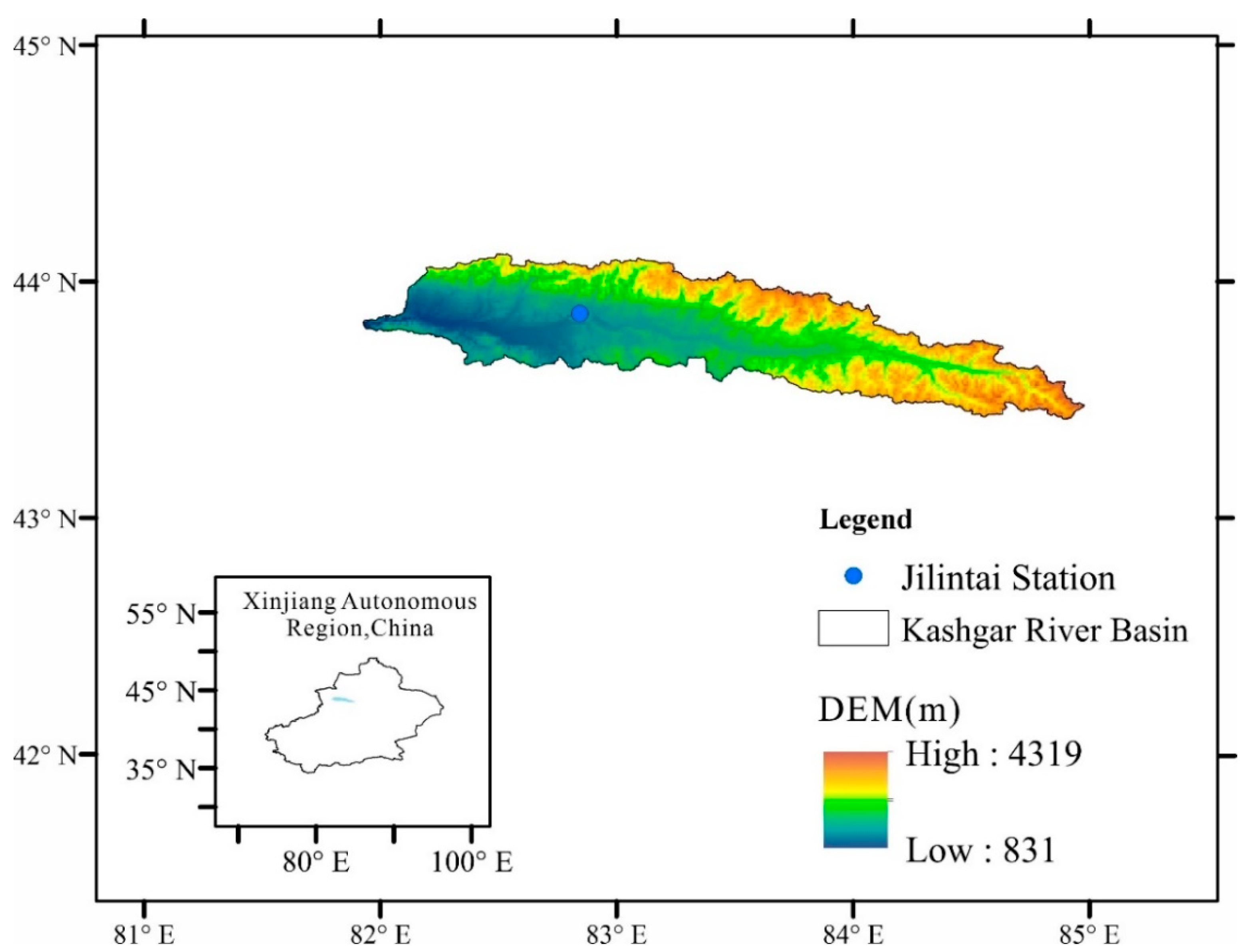
2. Study Area and Data

The Kashgar River Basin in Xinjiang is geographically situated between 81°50′ E to 84°45′ E and 43°25′ N to 44°20′ N latitude, encompassing a total area of 9578 km². The Kashgar River flows from east to west through Nileke County, veers south after passing through the Tuohai mountain exit, and finally joins the Ili River at Yama Ferry, with a total length of 297 km. The river system is characterized by a narrow, willow-leaf-shaped, pinnate pattern (see Figure 1). Located in the hinterland of the Eurasian continent, the Kashgar River is subject to a typical temperate continental arid climate. The basin has an average annual temperature of 5.7 °C and an average annual precipitation of 353.4 mm, with the maximum daily rainfall recorded at 33.4 mm and an average annual evaporation rate of 1471.8 mm. Recorded temperature extremes have reached a high of 37.9 °C and a low of −39.9 °C.

Streamflow data for this research were gathered daily from the Jilintai station. The study period spans from January 1961 to December 2015, selected based on data availability. The study utilizes input variables represented by the standardized anomaly values of several hydroclimatic factors. These include Temperature^t (${Tmp}^t$), Precipitation^t and Precipitation^t−1 (${Pre}^t$, ${Pre}^{t-1}$), Relative Humidity^t (${Rhm}^t$), Potential Evapotranspiration^t (${Pet}^t$), Vapour pressure^t (${Vap}^t$), Soil Moisture^t (${Sm}^t$), Terrestrial water storage^t (${Tws}^t$), Snow water equivalent (${Swe}^t$), and Streamflow^t (${Stf}^t$) with the superscript t denoting the specific time step. The predictive target is the following time step’s Streamflow^t+1 (${Stf}^{t+1}$) at the (t + 1) time step. The standardized anomaly values for each month are calculated by deducting the monthly mean from each data point and normalizing this figure using the standard deviation for that particular month. For this study, daily precipitation data were acquired from the Chinese National Meteorological Information Center, accessible at http://data.cma.cn/ (accessed on 20 March 2024). Precipitation data at monthly scale were transformed by accumulating daily data on each specific month. Gridded relative humidity, potential evapotranspiration and vapor pressure data were downloaded from the Climatic Research Unit (CRU) time series [26]. The monthly soil moisture, terrestrial water storage and snow water equivalent data were taken from Miao and Wang [27]. The hydrometeorological information was extracted from the above grid points located within the study basin.

3. Methodology

A systematic flowchart of the proposed nonstationary Graphical model (GM) and Bayesian networks-based model (NGM-BNs) is plotted in Figure 2. In comparison to the use of stationary GM-BNs with only one static network structure (bottom panel in Figure 2), NGM-BNs should consider a number of time-varying network structures corresponding to predictand–predictor association under nonstationary scenarios. As shown in Figure 2, M phases of nonstationary modelling of NGM-BNs were decided by predicting the time horizon (n). In this study, 15 years are used as size of testing periods, which represents that $\mathit{M}=⌊\frac{15}{\mathit{n}}⌋+1.$ Throughout the M phases of NGM-BNs modeling, various forms of dynamic network structures are discerned via GM-based Bayesian networks (BNs), which elucidate the interrelationships among numerous interdependent variables. In the final step, the variables that exert direct influence, commonly termed as the ‘parents’ of the target variables, are pinpointed within these nonstationary networks for integration into the evolving prediction models. In our proposed NGM-BNs model, it is crucial to establish a prediction time frame (n) beyond which the model requires updating to incorporate evolving characteristics. This timeframe should be carefully balanced, sufficiently extensive to capture temporal variations in associations, yet concise enough to prevent excessively frequent updates. Determining an optimal n-year period is key to achieving the most accurate predictive outcomes.

3.1. Bayesian Network-Based Prediction Models

The Bayesian network modeling workflow usually comprises three key phases: (1) determining the network architecture utilizing a graphical-model-based framework; (2) calculating the network’s parameters; and (3) conducting long-lead prediction of the target variable through the Bayesian network.

In this study, we deploy Bayesian networks (BNs) grounded in Graphical Modeling, executed using the ‘bnlearn’ package in R-Software (R-4.3.3) [28]. The optimization of the network’s structure is carried out through the Hill Climbing (HC) greedy search algorithm, a score-centric learning strategy. We use the Hill Climbing (HC) greedy search algorithm for the following reasons: (1) it is easy to implement and understand; (2) it has great efficiency in finding solution to the problem of a single peak or a smooth slope leading to the optimum; (3) it does not occupy much computer memory. Iterative updates to the graph’s structure are guided by the Bayesian Information Criterion (BIC) score, involving additions, deletions or alterations of edges, with a concurrent reassessment of the network score in each iteration. This score reflects the model’s fitting prowess, with the highest BIC score indicating optimal fit. Following the establishment of the network structure via the GM method, the next step is to evaluate the strength of the association between pairs of variables (nodes) linked by an edge, termed as edge strength, which is quantifiable through the BIC score. In our research, we have utilized the Bayesian Information Criterion (BIC) score for the purpose of selecting the model. The calculation of the BIC score proceeds as follows.

$$BIC=\sum _{i=1}^{n}log{F}_D\left(x_i|{\Lambda }_{X_i}\right)-\frac{d}{2}logN$$

(1)

The subscript D denotes the dataset; $F_D$ symbolizes the dataset’s joint probability distribution;${\Lambda }_{X_i}$ signifies the set of parent variables for $X_i$ within graph modelling result; d represents the count of parameters in the comprehensive distribution; N is the dataset’s size. The BIC score is an indicator of model adequacy: a higher score suggests a more accurate model representation. Consequently, the graph structure that yields the highest score is chosen.

Upon identifying the optimal network configuration and the corresponding parent variables, the parameters for the chosen network are determined using the maximum likelihood estimation (MLE) technique. Let {$X_1,X_2,\dots ,X_m\}$be a date set composed of m random variables corresponding to a certain network. The joint distribution of m random variables, often referred to as the overall data distribution, can be articulated in the following manner:

$$F\left(X_1,X_2,\dots ,X_m|\mathbf{\Theta }\right)=\prod _{i=1}^{m}F(X_i|{\Lambda }_{X_i},{\theta }_i)$$

(2)

where ${\theta }_i$ symbolizes the array of parameters governing the conditional distribution of $X_i$ given its set of precursors, ${\Lambda }_{X_i}$. This set, ${\Lambda }_{X_i}$, is essentially a collection of other random variables, also referred to as ‘parents’, which have a direct relationship with $X_i$. Collectively, these parameters are denoted as $\mathbf{\Theta }=\{{\theta }_1,{\theta }_2,\dots ,{\theta }_m\}$. The function $F(X_i|{\Lambda }_{X_i},{\theta }_i)$ represents the local distribution function, which is designed to demonstrate the interdependencies between $X_i$ and its associated parent variables. With the graphical structure of the network already delineated from a prior step, parameter estimation for these local distributions can be conducted with improved efficiency.

Upon the determination of parameters for both the global and local distribution functions, the Bayesian Network Model (BNM)-based predictive framework can be launched. Forecasting the desired variable is then achieved by substituting new values for the parent nodes into the local distribution function, these parent nodes are what we refer to as potential input variables.

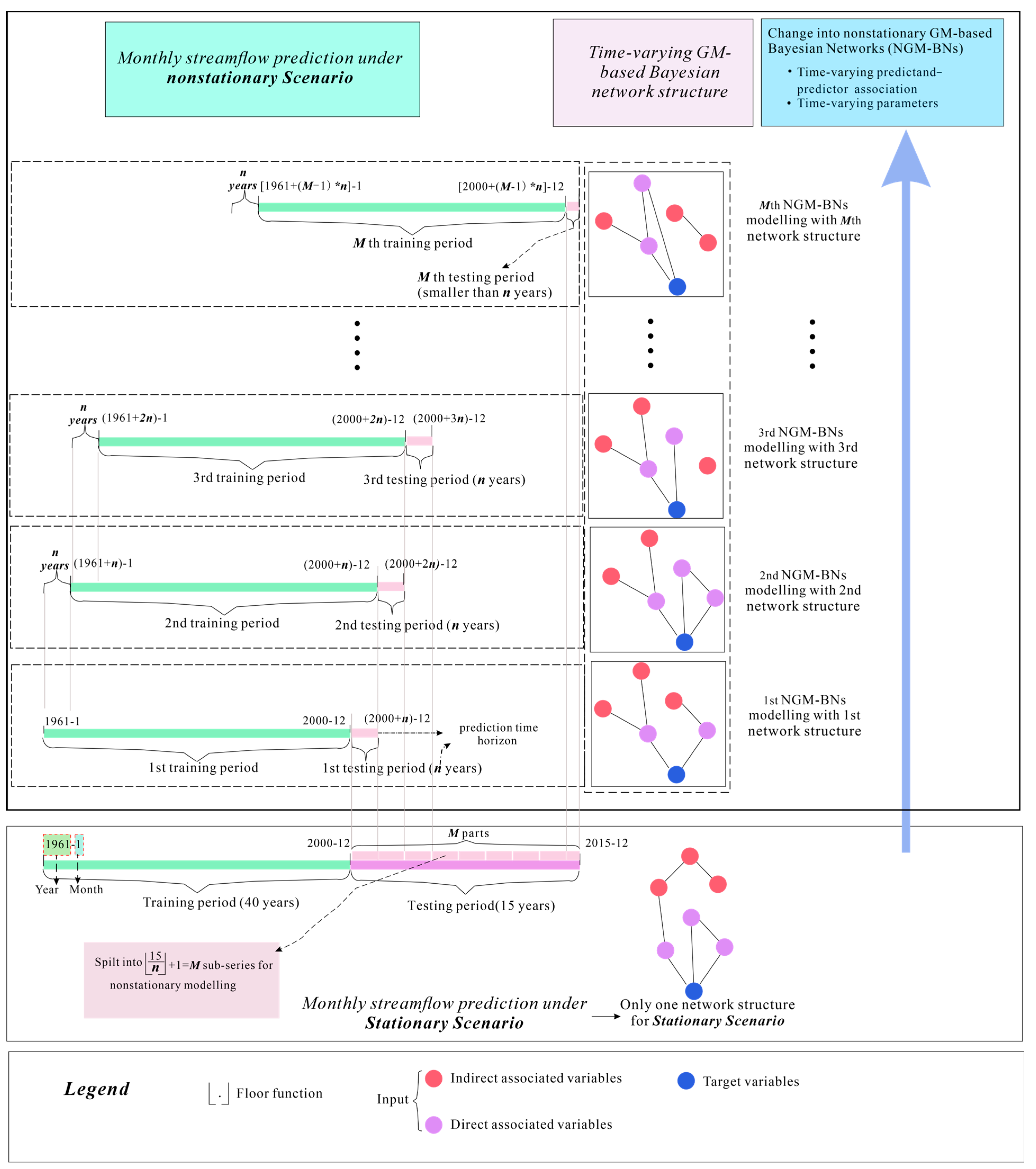
3.2. Identification of Dynamic Networks Based on Multiple Performance Metrics

The architecture of this network requires periodic modifications, creating a sequence of evolving structures that embody the notion of dynamic networks [29]. The optimal interval for these updates, known as the most suitable prediction time horizon (MST) for model recalibration and denoted by M, is determined by the optimal predictive accuracy of the probabilistic model in relation to the network structures identified. The underlying principle stems from the recognition that predictive accuracy tends to diminish over time. Consequently, the relevance of the initially identified network structure may wane due to potential temporal variations.

The duration of the model training phase and the fine-tuning of the MST for model recalibration are outlined as follows: The window for model development should be of sufficient length to establish a stable network structure, yet concise enough to accurately trace the dynamic interactions between inputs and outputs. Given that a 40-year span is generally accepted as a climatic period, the model development is hence framed within a sliding 40-year window. For example, assuming the MST is n years, we commence the initial training from 1961 to 2000, with the first testing period extending from 2001 to 2000 + n. Subsequent recalibrations, occurring every n years, prompt an n-year advancement in the development period, now from 1961 + n to 2000 + n, and a corresponding testing period from (2000 + n) + 1 to (2000 + 2n). This iterative process is maintained throughout the study’s entire duration. The objective is to refine the value of n to secure an MST that ensures the predictive model remains sensitive to significant temporal variations yet refrains from recalibrating too often, which would offer negligible improvements in predictability. To deduce the MST, this methodology is replicated over M phases, with the M chosen large enough to encompass the MST by the designer’s judgment. The performance of the model is then scrutinized across consecutive testing intervals, effectively assessing the period from 2001 to 2015 with varying n to determine the optimal frequency of model updates.

In order to evaluate performance of the proposed NGM-BNs model, five kinds of residue error analyzing metrics are used: (1) normalized root-mean-square error (nRMSE); (2) Kling–Gupta efficiency (KGE) [30]; (3) Nash–Sutcliffe efficiency coefficient (NSE); (4) index of agreement (d); and (5) coefficient of determination ($R^2$). These five metrics of the BNM-based prediction model are compared with those of the ANFIS-based prediction model and SVR-based prediction models.

4. Results

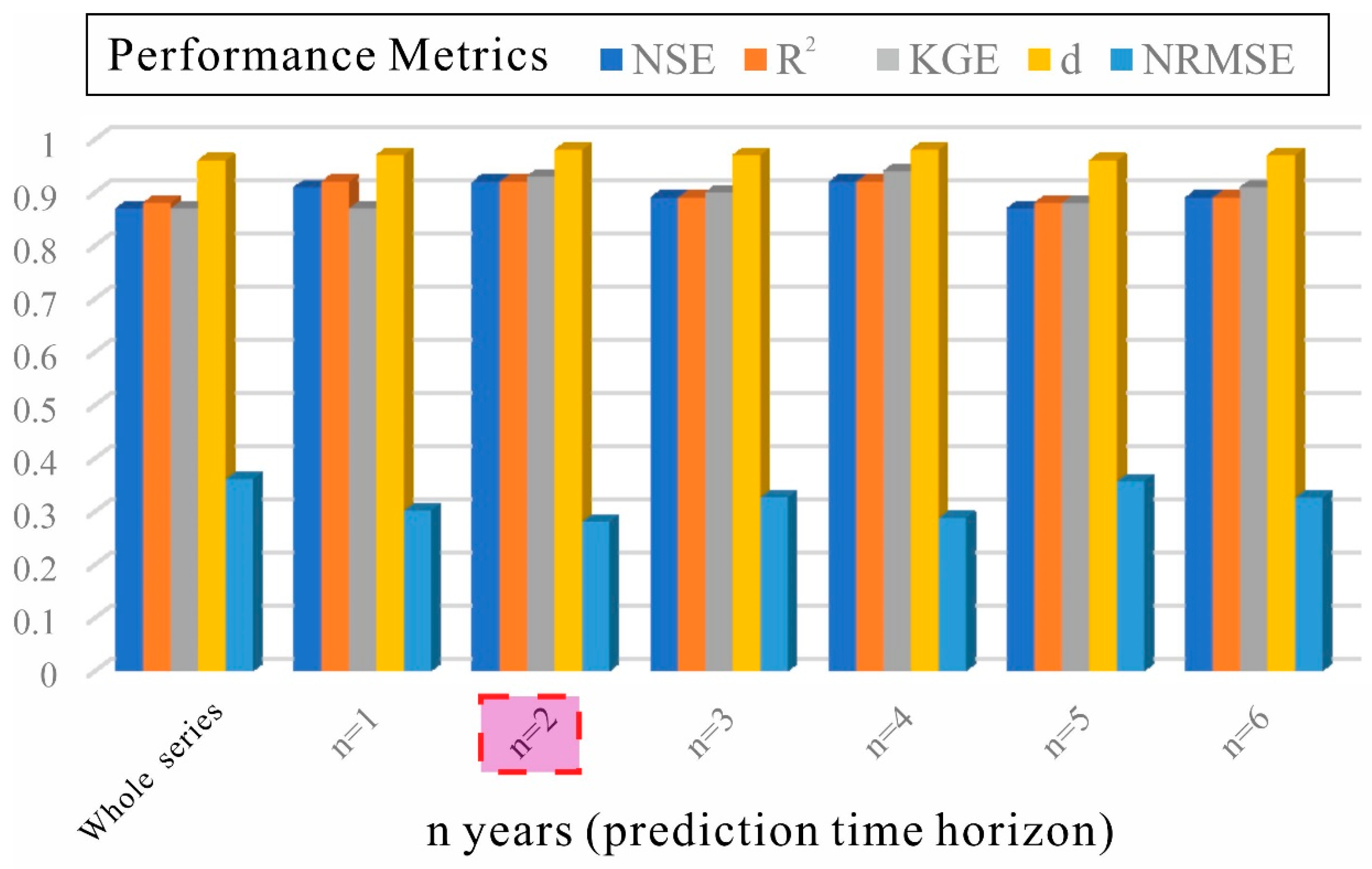
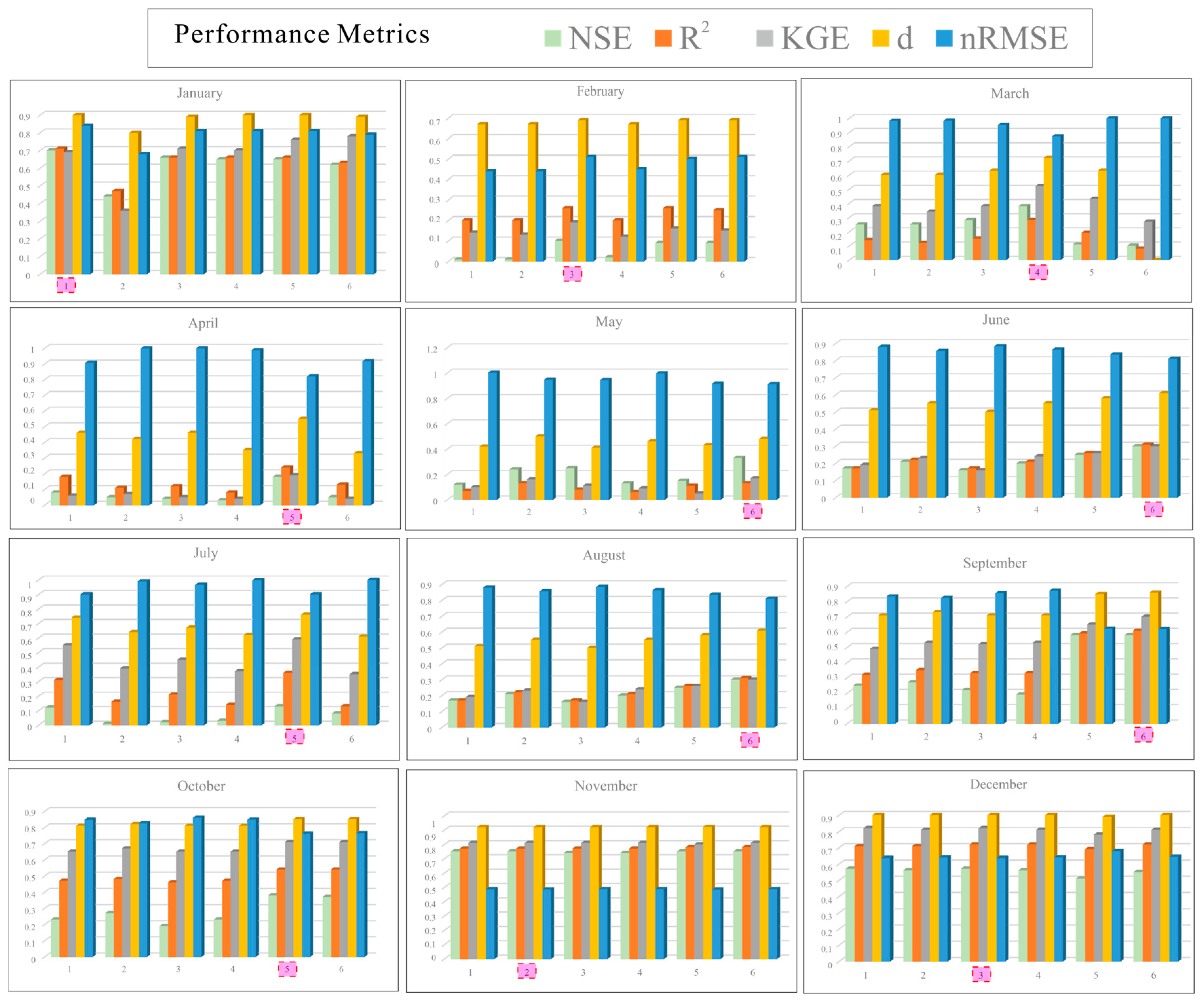
4.1. Determination of MST Based on Five Performance Metrics

Given the integration of nonstationarity within the monthly runoff forecasts in this study, it becomes essential to determine the most suitable prediction timeframe (spanning n years), after which the model requires an update to reflect the evolving temporal features.

In this study, each network structure during each model training period considering all the months together as a single time series was conducted, which means the models are not developed separately for different months of the year (month-wise strategy of prediction).

We employ a series of predetermined time spans, ranging from 1 to 6 years (i.e., $\mathit{n}=1, 2, \dots , 6$ years), as our forecasting intervals. For each interval, the training phase of the model encompasses a 40-year period. During each training phase, we construct a Bayesian network structure. Following this, a probabilistic model leveraging the network structure forecasts the standardized streamflow anomalies over the testing period. The forecast outcomes are then gathered for each 15-year testing phase, covering the years 2001 to 2015. As previously stated, the analysis proceeds for all potential values of n, with the most suitable prediction time horizon (MST) determined by the performance metrics (KGE, nRMSE, NSE, d, $R^2$). Figure 3 illustrates the changes in these performance metrics as n varies, comparing actual versus predicted streamflows. It clearly shows a marked decline in model efficacy beyond a certain threshold of n. The results from Figure 3 indicate that under stationary conditions, neglecting the time-varying nature of the predictand–predictor association (as shown in the ‘whole series’ in Figure 3), the performance metrics are NSE = 0.87, $R^2$ = 0.88, KGE = 0.87, d = 0.96 and nRMSE = 36.1%, which is poorer compared to those of nonstationary scenarios (n = 1,2, …,6). When considering non-stationary characteristics (the MST = 2 revealing it to be the most effective interval for accurate model forecasting), the positive-direction indicators (NSE, $R^2$, d, KGE) improved by 4% to 6%, while the negative-direction indicator (nRMSE) decreased by 23%.

After we have selected the MST as 2 years with the optimal performance metrics (the biggest value of NSE, $R^2$, d, KGE and the smallest value of nRMSE), the time-varying network structures obtained for this study are shown in Figure 4.

The network structure from the initial training phase (1961–2000) suggests that the antecedents influencing streamflow include the previous month’s streamflow, terrestrial water storage, and snow water equivalent. In this phase, the current month’s streamflow shows a dependency on the prior month’s flow. During the subsequent training interval (1963–2002), the identified precursors to streamflow expand to incorporate precipitation alongside terrestrial water storage and the previous month’s snow water equivalent. Here, the current month’s streamflow becomes conditionally independent of the previous one when factoring in the prior month’s precipitation.

As the analysis progresses to the third phase (1965–2004), precipitation, temperature and the previous month’s streamflow emerge as key streamflow predictors. In this instance, the current streamflow retains its dependence on the previous month’s metrics. For the fourth period (1967–2007), the network reveals terrestrial water storage, the prior month’s streamflow and temperature as influential factors.

Moving into the fifth phase (1969–2009), the focus narrows to terrestrial water storage and the preceding month’s streamflow as significant predictors. By the time we reach the 6th (1971–2011) and 7th (1973–2013) training periods, terrestrial water storage from the previous month stands out as the sole notable predictor, indicating a shift where variables tied to snowmelt increasingly drive the monthly streamflow forecasting in the Kashgar River Basin in more recent times. Potential evapotranspiration and atmospheric pressure are directly correlated with temperature. The final results of nonstationary GM and Bayesian networks-based models (NGM-BNs) using the most suitable prediction time horizon (MST) as 2 years are shown in

Table 1. Detailed information of the nonstationary GM and Bayesian-networks-based models (NGM-BNs) using most suitable prediction time horizon (MST) as 2 years.

Sub-Series	Training Period	Testing Period	NGM-BNs
1	1961–2000	2001–2002	$f(y|{Swe}^t,{Tws}^t,{Stf}^t)$
2	1963–2002	2003–2004	$f(y|{Pre}^t,{Tws}^t,{Swe}^t)$
3	1965–2004	2005–2006	$f(y|{Pre}^t,{Tmp}^t,{Stf}^t)$
4	1967–2006	2007–2008	$f(y|{Tws}^t,{Tmp}^t,{Stf}^t)$
5	1969–2008	2009–2010	$f(y|{Tws}^t,{Stf}^t)$
6	1971–2010	2011–2012	$f(y|{Tws}^t)$
7	1973–2012	2013–2014	$f(y|{Tws}^t)$
8	1975–2014	2015	$f(y|{Tws}^t,{Stf}^t)$

Note: Notations for the variables are as follows: Temperature^t (${Tmp}^t$), Precipitation^t and Precipitation^t−1 (${Pre}^t$, ${Pre}^{t-1}$), Potential Evapotranspiration^t (${Pet}^t$), Relative Humidity^t (${Rhm}^t$), Vapour pressure^t (${Vap}^t$), Soil Moisture^t (${Sm}^t$), Terrestrial water storage^t (${Tws}^t$), snow water equivalent (${Swe}^t$), and Streamflow^t (${Stf}^t$) are the input variables and Streamflow^t+1 (y) is the target variable.

.

Here, we also developed the NGM-BN models separately for different months of the year considering cyclostationarity, which is called a month-wise strategy of prediction [31]. The corresponding results are shown in Figure 5 and Figure 6 and

Table 2. Detailed information of the nonstationary GM and Bayesian networks-based models (NGM-BNs) for March–October based on month-wise prediction strategy.

Training Period (Testing Period)	NGM-BNs
	MST = 6
	May	June		August		September
1961–2000 (2001–2006)	$f(y|{Stf}^t)$	$f(y|{Tws}^t)$		$f(y|{Pre}^t,{Stf}^t)$		$f(y|{Tws}^t,{Stf}^t)$
1967–2006 (2007–2012)	$f(y|{Stf}^t)$	$f(y|{{Tmp}^t,Stf}^t)$		$f(y|{Stf}^t)$		$f(y|{Stf}^t)$
1973–2012 (2013–2015)	$f(y|{Swe}^t,{Stf}^t)$	$f(y|{Pet}^t,{Stf}^t)$		$f(y|{Swe}^t,{Stf}^t)$		$f(y|{Pet}^t,{Stf}^t)$
Training period (Testing period)	MST = 5
	April		July		October
1961–2000 (2001–2005)	$f(y|{{Pet}^t,Stf}^t)$		$f(y|{Pre}^t)$		$f(y|{Stf}^t)$
1966–2005 (2006–2010)	$f(y|{{Tmp}^t,Stf}^t)$		$f(y|{Stf}^t)$		$f(y|{Pre}^t)$
1971–2012 (2011–2015)	$f(y|{Swe}^t)$		$f(y|{Swe}^t,{Stf}^t)$		$f(y|{Stf}^t)$
Training period (Testing period)	MST = 4
	March
1961–2000 (2001–2004)	$f(y|{Stf}^t)$
1965–2004 (2005–2008)	$f(y|{{Pet}^t,Stf}^t)$
1969–2008 (2009–2012)	$f(y|{Swe}^t)$
1973–2012 (2013–2015)	$f(y|{{Tws}^t,Stf}^t)$

. Different from the non-month-wise strategy used in this study, which developed nonstationary network structure considering all the months together as a single time series, the MST value of month-wise prediction strategy (Figure 5) was different for each month (1 for January, 2 for November, 3 for February and December, 4 for March, 5 for April, July and October, 6 for June, August and September). As shown in Figure 6, the number of potential associations under month-wise strategy between variables was smaller than those in Figure 4. Taking February as an example, the performance metrics of February derived from the month-wise strategy (NSE = 0.09, $R^2$ = 0.25, KGE = 0.18, d = 0.68 and nRMSE = 50%) were poorer than those of the non-month-wise strategy used in this study. The sample size from the month-wise strategy was only 40, while the sample size from the non-month-wise strategy (creating a dynamic network framework that treated the data from all months as a unified time series) was 480. So, the results of the Bayesian network structure in this study were more robust than those derived from the month-wise strategy.

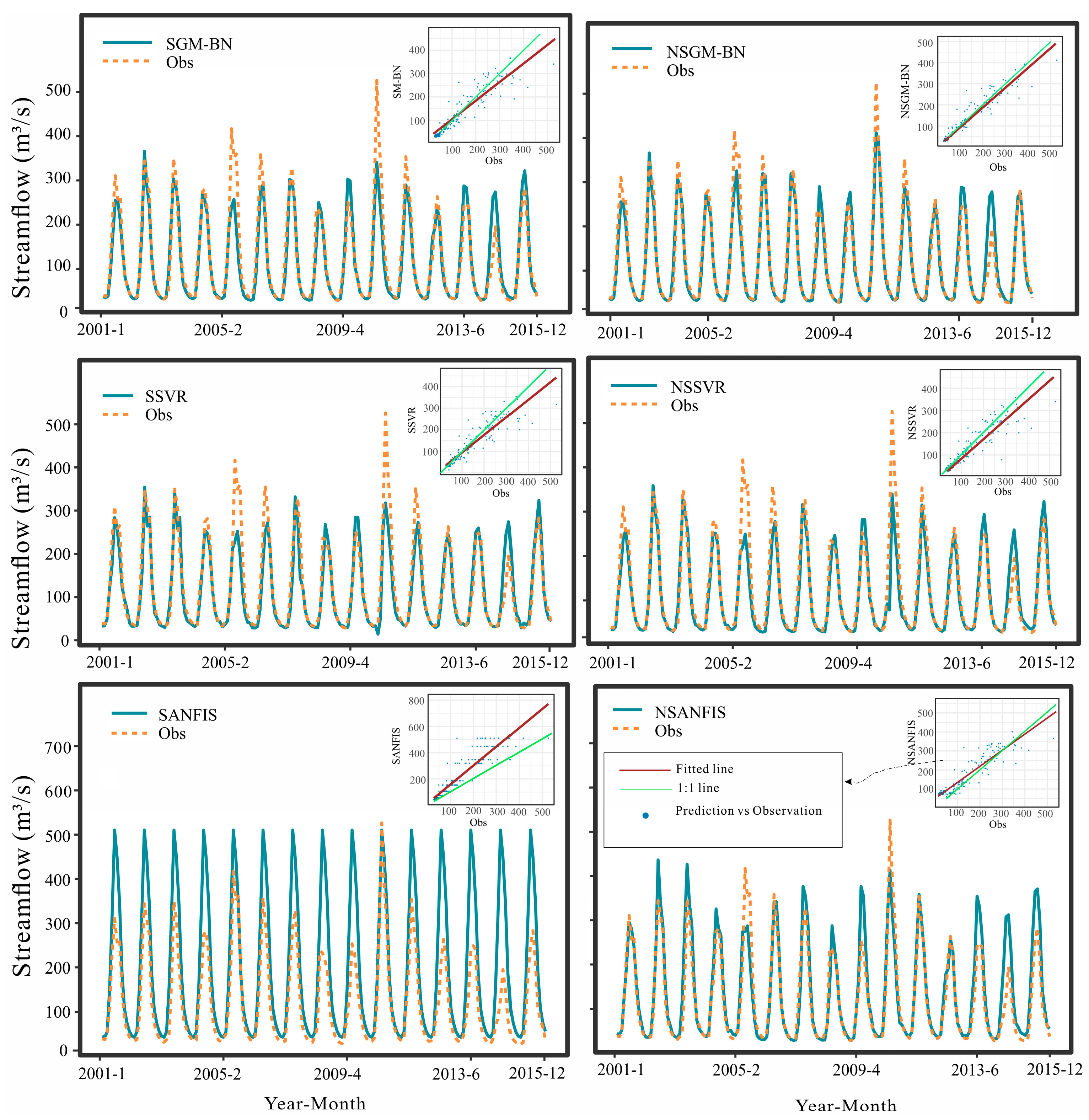
4.2. Comparison of Performance of the Nonstationary Bayesian Network-Based Model with Other Data-Driven Models

The time series plots and scatter diagrams in Figure 7 display the recorded and forecasted monthly streamflow at Jilintai stations, derived from various models. These visualizations facilitate a comparative analysis of the predictive accuracy of the NGM-BN model against other methodologies. We have quantified different performance metrics and presented them in

Table 3. Results of various performance metrics evaluated for different models during the model testing period from 2001 to 2015.

Performance Metrics	Models
	Nonstationary GM-BN	Stationary GM-BN	Nonstationary SVR	Stationary SVR	Nonstationary ANFIS	Stationary ANFIS
R2		0.88	0.86	0.43	0.86	0.86
nRMSE	0.281	0.361	0.388	0.892	0.422	0.98
NSE	0.93	0.87	0.85	0.20	0.82	0.03
d	0.98	0.96	0.96	0.80	0.96	0.86
KGE	0.94	0.87	0.84	0.62	0.85	0.22

for each model evaluated. For the proposed NGM-BN model (illustrated in the top right panel of Figure 7), the alignment between observed and predicted streamflow is quantified as follows: NSE = 0.93, $R^2$ = 0.92, KGE = 0.94, d = 0.98, and nRMSE = 28.1%. An inspection of Figure 7 indicates that the NGM-BN model adeptly captures streamflow across a range of flows. However, the model’s accuracy fluctuates throughout the year, with more pronounced errors during periods of higher flow. Presenting the data collectively for all months conceals these monthly discrepancies. Additionally, peak streamflow events in 2006, 2010 and 2012 were consistently underestimated, while those in 2002 and 2013 were overestimated by most models. Precipitation, a key factor during months of high flow, can lead to overestimation or underestimation of streamflow if the actual precipitation deviates from the average. Nonetheless, congruence between rainfall variations and streamflow is not always guaranteed due to other influences such as the wetness condition of the catchment, changes in land use and cover and evolving terrestrial dynamics. For instance, a drier system often weakens the correlation between rainfall and streamflow. Similarly, gradual shifts in land use and terrestrial conditions can alter this relationship over time, resulting in a dynamic association. Moreover, changes in soil moisture, evaporation rates, snowmelt-related indexes and other atmospheric variables might further affect the level of synchrony between rainfall and streamflow.

In Figure 7, the top left panel illustrates the predictive capabilities of the stationary-network-based model. This model’s performance in exhibiting the divergence between observed and predicted streamflow is quantified by the following metrics: NSE = 0.87, $R^2$ = 0.88, KGE = 0.87, d = 0.96, and nRMSE = 36.1%. The stationary GM-BN model demonstrates a notable ability to replicate low-flow events, nearly matching the performance of temporal-network-based methods. Yet, the latter, specifically the proposed nonstationary NGM-BN-based approach, excels in capturing high-flow scenarios. This superior performance in both high- and low-flow situations highlights the overall effectiveness of the temporal-network-based approach over the conventional time-invariant model. This advantage is particularly relevant in the context of nonstationarity, as many basins are experiencing shifts in interannual streamflow variability, positioning temporal networks as a viable alternative.

The results for Support Vector Regression (SVR) are depicted in Figure 7, specifically in the third (stationary; middle left panel) and fourth (nonstationary; middle right panel) panels. Analogously, the Adaptive Neuro-Fuzzy Inference System (ANFIS) outcomes are presented in the fifth (stationary; bottom left panel) and sixth (nonstationary; bottom right panel) panels. The detailed parameter settings of SVR and ANFIS are exhibited in Tables S1 and S2.

The analysis reveals that both SVR and ANFIS models with nonstationary frameworks outperform their stationary versions. The nonstationary SVR, in particular, manages satisfactory results for average and low-flow periods but struggles significantly with high-flow predictions. The performance of the stationary SVR model is even less impressive. When comparing network-based approaches, as shown in Table 3, the nonstationary variant (top right panel of Figure 7) excels over the time-invariant SVR models. Table 3 conveniently consolidates performance metrics for all four models, facilitating straightforward comparison. In summary, a comprehensive evaluation of the different methods strongly supports the adoption of the proposed nonstationary-network-based approach.

Consolidating the findings, it becomes clear that the relationships between hydroclimatic variables are not static but evolve over time. Given that stationary models assume a fixed relationship between dependent and independent variables, their predictive accuracy is inherently limited. Conversely, accurately determining the dynamic interplay among the variables is key to enhancing model performance. This study confirms the superior predictive capability of the proposed nonstationary-network-based approach, which acknowledges and leverages these time-varying connections. The advantages of this approach are especially pertinent in the context of a changing climate where the assumption of stationarity is increasingly unreliable. Therefore, the nonstationary-network-based method is advocated as a promising alternative for hydroclimatic modeling under such conditions.

5. Discussion

This study introduces dynamic Bayesian networks as a robust methodology for hydrometeorological forecasting, designed to address the evolving dynamics of a system with interconnected variables. Traditional modeling often relies on the assumption of static relationships. Yet, the necessity to account for nonstationarity, driven by changing terrestrial and climatic conditions, is increasingly evident. This work not only presents but also validates the efficacy of a novel network-based strategy that incorporates nonstationarity into hydroclimatic analysis. Leveraging the capabilities of Nonstationary Graphical Models and Bayesian Networks (NGM-BNs), this study develops adaptive, time-sensitive predictive models that reflect the hydroclimatic system’s temporal variations.

This study further argues that the network structures may evolve over time, reflecting the dynamic nature of the system. Consequently, the approach advocated here involves periodic updates to both the network structures and the model’s predictive parameters at regular intervals, referred to as the most suitable prediction time horizon (MST), to accurately reflect these changes. In this study, the value of MST is identified as 2 years for non-month-wise strategy prediction, which develops nonstationary network structure considering all the months together as a single time series. The MST value of the month-wise prediction strategy (Figure 5) was different for each month (1 for January, 2 for November, 3 for February and December, 4 for March, 5 for April, July and October, 6 for June, August and September). Due to the poor performance of the month-wise prediction strategy (NSE = 0.09, $R^2$ = 0.25, KGE = 0.18, d = 0.68 and nRMSE = 50%), the non-month-wise strategy prediction was adopted in this study.

Since the length of the time series was definitely a potential factor influencing the performance of the proposed NGM-BNs model, we used another basin of China, the Huaihe River Basin, which has a sample size of 804, to reverify its wide applicability. The compared results of the nonstationary Bayesian Network model and stationary models are shown in Table S3. Not only are the performance metrics of the nonstationary Bayesian network models significantly better than those of the stationary models (NSE = 0.96, $R^2$ = 0.97, KGE = 0.97, d = 0.98 and nRMSE = 22.5%), but the predictive capabilities of the other two data-driven models (SVR and ANFIS) have also been significantly improved due to the increase in sample size. Although our study focused more on the incorporation of nonstationarity to enhance the predicting accuracy of Bayesian Network models, it is also beneficial to ensure enough dataset size to improve the ability of the proposed model. If the sample size is very low, the performance of the proposed NGM-BNs model would be definitely influenced. As a result, the NGM-BNs-based monthly streamflow forecasting should have more abundant data in the future.

6. Conclusions

This study focuses on the hydroclimatic modeling of monthly streamflow, which involves a number of interrelated variables that interact in complex patterns, exemplifying the utility of the proposed method. We have achieved the following conclusions:

(1)

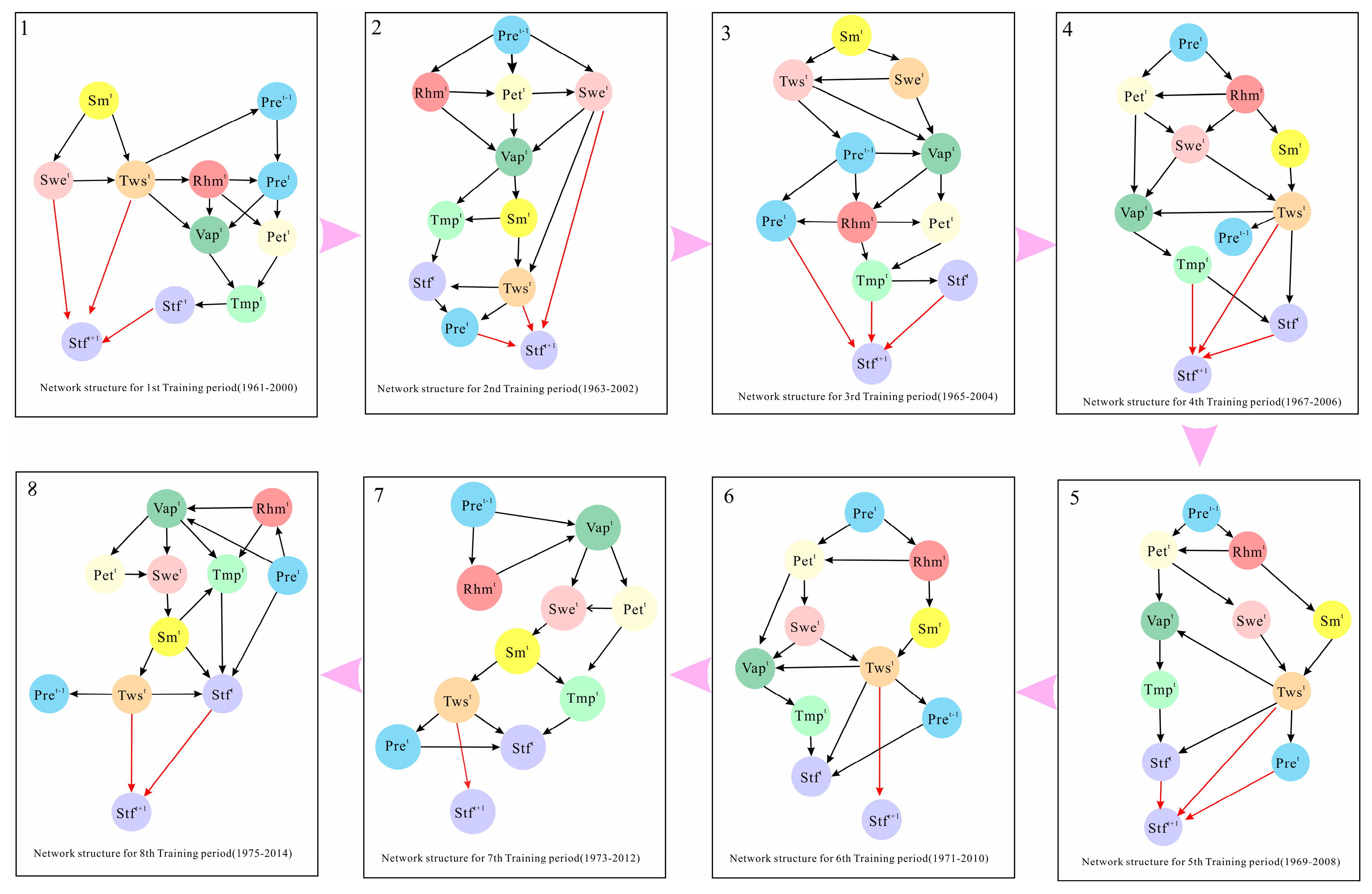
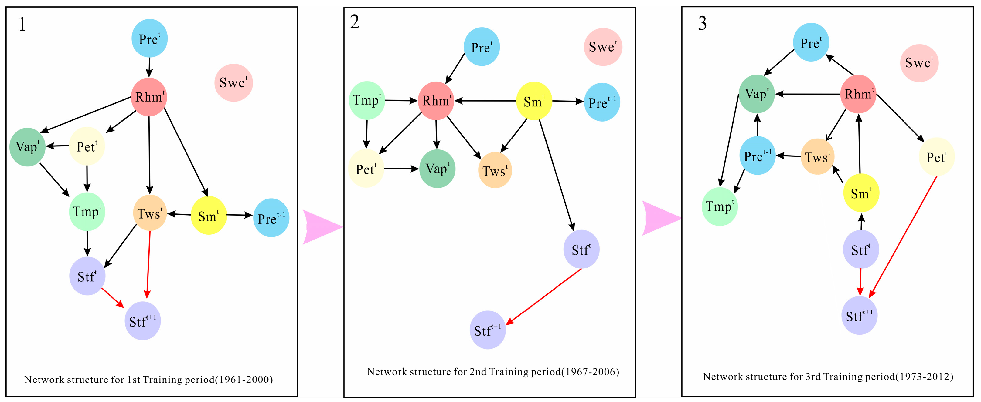
Utilizing this approach, we uncover network structures that accurately map the dependencies among these variables. Analysis of the network configurations indicates a robust link between the streamflow of the current month and that of the preceding month in most cases.

(2)

In the later stages of network structure analysis (specifically the 6th and 7th phases of this study), it becomes apparent that the previous month’s terrestrial water storage emerges as a singular significant predictor. This suggests that, against the background of climate change, factors related to snowmelt have taken on a more pronounced role in determining the monthly streamflow within the Kashgar River Basin in recent periods.

(3)

Employing the nonstationary-network-based approach yields significantly enhanced outcomes in comparison to static models, capturing the nuances of both high- and low-flow occurrences with greater fidelity.

(4)

Across the board, it is evident that approaches incorporating nonstationarity consistently outperformed their stationary equivalents. This underscores the superior performance of models that adjust over time, with the proposed network-based models leading the pack due to their capacity to accommodate the dynamic correlations among hydroclimatic factors. The strength of the proposed model lies in its adeptness at capturing both extremes of flow magnitudes, which not only exemplifies its precision but also suggests its potential utility in enhancing water resource management.

References

1. Betterle, A.; Radny, D.; Schirmer, M.; Botter, G. What do they have in common? Drivers of streamflow spatial correlation and prediction of flow regimes in ungauged locations. Water Resour. Res. 2017, 53, 10354–10373. [Google Scholar] [CrossRef]
2. Reddy, N.M.; Saravanan, S.; Almohamad, H.; Al Dughairi, A.A.; Abdo, H.G. Effects of climate change on streamflow in the Godavari Basin simulated using a conceptual model including CMIP6 dataset. Water 2023, 15, 1701. [Google Scholar] [CrossRef]
3. McInerney, D.; Thyer, M.; Kavetski, D.; Laugesen, R.; Woldemeskel, F.; Tuteja, N.; Kuczera, G. Seamless streamflow forecasting at daily to monthly scales: MuTHRE lets you have your cake and eat it too. Hydrol. Earth Syst. Sci. 2022, 26, 5669–5683. [Google Scholar] [CrossRef]
4. Ahn, K.H.; Yellen, B.; Steinschneider, S. Dynamic linear models to explore time-varying suspended sediment-discharge rating curves. Water Resour. Res. 2017, 53, 4802–4820. [Google Scholar] [CrossRef]
5. Ferguson, C.R.; Pan, M.; Taikan, O. The effect of global warming on future water availability: CMIP5 synthesis. Water Resour. Res. 2018, 54, 7791–7819. [Google Scholar] [CrossRef]
6. Tian, P.; Feng, J.H.; Zhao, G.J.; Gao, P.; Sun, W.Y.; Hörmann, G.; Mu, X. Rainfall, runoff, and suspended sediment dynamics at the flood event scale in a Loess Plateau watershed, China. Hydrol. Process. 2022, 36, e14486. [Google Scholar] [CrossRef]
7. Yoosefdoost, I.; Khashei-Siuki, A.; Tabari, H.; Mohammadrezapour, O. Runoff simulation under future climate change conditions: Performance comparison of data-mining algorithms and conceptual models. Water Resour. Manag. 2022, 36, 1191–1215. [Google Scholar] [CrossRef]
8. Carter, E.; Steinschneider, S. Hydroclimatological drivers of extreme floods on Lake Ontario. Water Resour. Res. 2018, 54, 4461–4478. [Google Scholar] [CrossRef]
9. Nakhaei, M.; Ghazban, F.; Nakhaei, P.; Gheibi, M.; Waclawek, S.; Ahmadi, M. Successive-station streamflow prediction and precipitation uncertainty analysis in the Zarrineh River Basin using a machine learning technique. Water 2023, 15, 999. [Google Scholar] [CrossRef]
10. Hao, Z.; Singh, V.P.; Xia, Y. Seasonal drought prediction: Advances, challenges, and future prospects. Rev. Geophys. 2018, 56, 108–141. [Google Scholar] [CrossRef]
11. Prakash, V.; Mishra, V. Soil mosture and streamflow data assimilation for streamflow prediction in the Narmada River Basin. J. Hydrometeorol. 2023, 24, 1377–1392. [Google Scholar] [CrossRef]
12. Kim, K.B.; Kwon, H.H.; Han, D. Exploration of warm-up period in conceptual hydrological modelling. J. Hydrol. 2018, 556, 194–210. [Google Scholar] [CrossRef]
13. Traveria, M.; Escribano, A.; Palomo, P. Statistical wind forecast for Reus airport. Meteorol. Appl. 2010, 17, 485–495. [Google Scholar] [CrossRef]
14. Ihler, A.T.; Kirshner, S.; Ghil, M.; Robertson, A.W.; Smyth, P. Graphical models for statistical inference and data assimilation. Physica D 2007, 230, 72–87. [Google Scholar] [CrossRef]
15. Jordan, M.I. Graphical models. Stat. Sci. 2004, 19, 140–155. [Google Scholar] [CrossRef]
16. Bracken, C.; Holman, K.D.; Rajagopalan, B.; Moradkhani, H. A Bayesian hierarchical approach to multivariate nonstationary hydrologic frequency analysis. Water Resour. Res. 2018, 54, 243–255. [Google Scholar] [CrossRef]
17. Dyer, F.; ElSawah, S.; Croke, B.; Griffiths, R.; Harrison, E.; Lucena-Moya, P.; Jakeman, A. The effects of climate change on ecologically-relevant flow regime and water quality attributes. Stoch. Env. Res. Risk A 2014, 28, 67–82. [Google Scholar] [CrossRef]
18. Morrison, R.; Stone, M. Spatially implemented Bayesian network model to assess environmental impacts of water management. Water Resour. Res. 2014, 50, 8107–8124. [Google Scholar] [CrossRef]
19. Tsonis, A.A.; Swanson, K.L.; Roebber, P.J. What do networks have to do with climate? Bull. Am. Meteorol. Soc. 2006, 87, 585–595. [Google Scholar] [CrossRef]
20. Ramadas, M.; Maity, R.; Ojha, R.; Govindaraju, R.S. Predictor selection for streamflows using a graphical modeling approach. Stoch. Env. Res. Risk A 2015, 29, 1583–1599. [Google Scholar] [CrossRef]
21. Ramadas, M.; Govindaraju, R.S. Probabilistic assessment of agricultural droughts using graphical models. J. Hydrol. 2015, 526, 151–163. [Google Scholar] [CrossRef]
22. Halverson, M.J.; Fleming, S.W. Complex network theory, streamflow, and hydrometric monitoring system design. Hydrol. Earth Syst. Sc. 2015, 19, 3301–3318. [Google Scholar] [CrossRef]
23. Phillips, J.D.; Schwanghart, W.; Heckmann, T. Graph theory in the geosciences. Earth-Sci. Rev. 2015, 143, 147–160. [Google Scholar] [CrossRef]
24. Nourani, V.; Komasi, M.; Mano, A. A multivariate ANN-wavelet approach for rainfall–runoff modeling. Water Resour. Manag. 2009, 23, 2877–2894. [Google Scholar] [CrossRef]
25. Maity, R.; Bhagwat, P.P.; Bhatnagar, A. Potential of support vector regression for prediction of monthly streamflow using endogenous property. Hydrol. Process. 2010, 24, 917–923. [Google Scholar] [CrossRef]
26. Harris, I.; Jones, P.D.; Osborn, T.J.; Lister, D.H. Updated high-resolution grids of monthly climatic observations-The CRU TS3.10 Dataset. Int. J. Climatol. 2013, 34, 623–642. [Google Scholar] [CrossRef]
27. Miao, Y.; Wang, A. A daily 0.25° × 0.25° hydrologically based land surface flux dataset for conterminous China, 1961–2017. J. Hydrol. 2020, 590, 125413. [Google Scholar] [CrossRef]
28. Scutari, M. Learning Bayesian Networks with the bnlearn R Package. J. Stat. Softw. 2010, 35, 1–22. [Google Scholar] [CrossRef]
29. Li, A.; Cornelius, S.P.; Liu, Y.Y.; Wang, L.; Barabási, A.L. The fundamental advantages of temporal networks. Science 2017, 358, 1042–1046. [Google Scholar] [CrossRef]
30. Kling, H.; Fuchs, M.; Paulin, M. Runoff conditions in the upper Danube basin under an ensemble of climate change scenarios. J. Hydrol. 2012, 424, 264–277. [Google Scholar] [CrossRef]
31. Dutta, R.; Maity, R. Temporal networks-based approach for nonstationary hydroclimatic modeling and its demonstration with streamflow prediction. Water Resour. Res. 2020, 56, e2020WR027086. [Google Scholar] [CrossRef]
Figure 1. Overview of the study region.
Water 16 01064 g001
Figure 2. The methodological framework illustrates the creation of a streamflow prediction model grounded in the principle of nonstationary (time-variant) networks. A rolling window of 40 years is designated as the training period, followed by n subsequent years as the testing period. The network configurations and model parameters undergo a process of updating at predetermined intervals, corresponding to the optimal n value. This interval is identified as the most suitable prediction time horizon (MST), which necessitates M times of model recalibration.
Water 16 01064 g002
Figure 3. Determining of the most suitable prediction time horizon (MST) for the dynamic GM-BN model. We conducted monthly streamflow predictions for the test period of 2001–2015, utilizing the time-varying GM-BN model. This analysis spanned forecast timeframes ranging from 1 to 6 years to identify the MST. Illustrated through a grouped bar chart, various performance metrics for the outcomes predicted at each timeframe were examined. The results clearly highlight a 2-year period as the MST, revealing it to be the most effective interval for accurate model forecasting. The prediction period marked in pink is the optimal prediction time horizon.
Water 16 01064 g003
Figure 4. The final time-varying network structure with most suitable prediction time horizon (MST) being two. The network structure was constructed by treating the data from all the months as a unified time series, providing a consolidated view of the temporal relationships. Notations for the variables are as follows: Temperaturet ( T m p t ), Precipitationt and Precipitationt−1 ( P r e t , P r e t 1 ), Potential Evapotranspirationt ( P e t t ), Relative Humidityt ( R h m t ), Vapour pressuret ( V a p t ), Soil Moisturet ( S m t ), Terrestrial water storaget ( T w s t ), Snow water equivalent ( S w e t ), and Streamflowt ( S t f t ) are the input variables, and Streamflowt+1 (y) is the target variable. The potential predictive relationships between the input variables and the targeted outcomes are highlighted in red to denote the final decision of input variables. The indirect predictive relationships between the input variables and the targeted outcomes are marked in black arrows.
Water 16 01064 g004
Figure 5. Determining of the most suitable prediction time horizon (MST) for the dynamic GM-BN model through month-wise forecasting strategy. We conducted monthly streamflow predictions for the test period of 2001–2015, utilizing the time-varying GM-BN model. This analysis spanned forecast timeframes ranging from 1 to 6 years to identify the MST. The prediction period marked in pink is the optimal prediction time horizon.
Water 16 01064 g005
Figure 6. The final time-varying network structure with most suitable prediction time horizon (MST) being 6 for September streamflow forecasting using month-wise strategy. Month-wise strategy of streamflow prediction was executed on a month-by-month basis by applying Bayesian network modeling to each month’s data series, which means 12 final Bayesian network structure was derived for 12 months under stationary cases. Notations for the variables are as follows: Temperaturet ( T m p t ), Precipitationt and Precipitationt−1 ( P r e t , P r e t 1 ), Potential Evapotranspirationt ( P e t t ), Relative Humidityt ( R h m t ), Vapour pressuret ( V a p t ), Soil Moisturet ( S m t ), Terrestrial water storaget ( T w s t ), snow water equivalent ( S w e t ), and Streamflowt ( S t f t ) are the input variables and Streamflowt+1 (y) is the target variable. The potential predictive relationships between the input variables and the targeted outcomes are highlighted in red to denote the final decision of input variables. The indirect predictive relationships between the input variables and the targeted outcomes are marked in black arrows.
Water 16 01064 g006
Figure 7. The comparative analysis juxtaposes the observed streamflow data against predictions derived from several methodologies: the proposed non-stationary Bayesian-networks-based approach, the traditional stationary-network-based approach, the adaptive non-stationary SVR (Support Vector Regression) approach, its stationary SVR-based counterpart, and both the dynamic non-stationary ANFIS (Adaptive Neuro-Fuzzy Inference System) approach and its stationary ANFIS-based variation.
Water 16 01064 g007