Hydrodynamic Characterization of Carbonate Aquifers Using Atypical Pumping Tests without the Interruption of the Drinking Water Supply

Abstract

The Gran Sasso carbonate aquifer is the largest and most productive in the Apennines. Its hydrogeological structure has been studied since the middle of the last century for the springs’ characterization for drinking purposes and for a motorway tunnel. Meanwhile, its hydrodynamic parametrization is less developed and has been limited to monitoring the discharge and chemical and isotopic parameters. Secondary porosity characterizes the aquifer, and an underlying impermeable marly complex represents the basal aquiclude. It might appear inappropriate to characterize the hydraulic properties via pumping tests, as their reliability has been proven in homogeneous and isotropic media. However, the high extent of the aquifer, the wells’ location, the scarcity of information available and the lack of alternatives has forced the estimation of hydrodynamic parameters as in porous aquifers and the experimental testing of the aquifer, especially in maximum pumping conditions, for a possible exploitation increase. Since aquifer testing was performed during the normal well field’s activities, it was not possible to perform typical tests. Therefore, the step-drawdown test was conducted by turning on an increasing number of wells over time and keeping the observation points fixed. As results, a mean hydraulic conductivity of 5 × 10⁻³ m/s and a mean transmissivity of 0.3 m²/s were established without interrupting the water supply; meanwhile, the influence radius and flow directions were also estimated.

1. Introduction

Carbonate fractured aquifers are used for groundwater supply in several regions of the world [1]; however, the characterization of their hydrodynamic properties is always challenging.

The use of the carbonate aquifers of the Central Apennines began during the 1960s and 1970s for big aqueducts serving millions of people. During that period, the Italian government set up an organization (“Cassa per il Mezzogiorno”) for research, study, and the exploitation of springs for drinking purposes [2,3,4]. Considerable economic resources were used for boreholes, and in some cases pumping tests for aquifer characterization were executed.

During the 1980s, 1990s, and 2000s, following the increased demand for drinking water, the use of the Apennine carbonate aquifers was implemented; consequently, many wells were built thanks to the high availability of groundwater [5], but with lower scientific precision than that of the “Cassa per il Mezzogiorno”.

Nowadays, regulations about groundwater and the increasing sensibility about the sustainable use of water resources, as well as the influence of climate change on groundwater [6,7,8], require a greater and deeper hydrogeological and hydrodynamic knowledge of aquifers. On the other hand, this necessity is contrasted by the logistical and economic unavailability of managing authorities for the execution of pumping tests; the logistical issues are due to the impossibility of halting water withdrawal and the distribution of drinking water.

This study aims to contribute to efforts to tackle the described issue, which is typical for the entire Central-Southern Apennines, using the same existing well field set-up. Moreover, this work will suggest a method for hydraulic conductivity and transmissivity estimation in carbonate aquifers to be applied for a potential exploitation increase. The hydraulic feature assessment can be useful for groundwater management, for the evaluation of the maximum exploitable amount, for the impact on the groundwater reservoir, and for the influence radius due to withdrawals.

The case study is about the Gran Sasso aquifer, one of the most important in Central Italy [5], which has been studied for engineering purposes and for the springs’ characterization; from a hydrodynamic point of view, the available data refer only to discharge, chemical, and isotopic features. The aquifer can be considered the most representative karst aquifer of the central-southern Apennines, with an extension of approximately 1000 km², a 700 mm/year an infiltration rate, and a total discharge ranging from 18 to 25 m³/s [9,10] with 3.5 m³/s exploited for drinking purposes. The lack of hydrodynamic data and the presence of well fields have allowed the execution of atypical step-drawdown tests using the exploited wells, both for pumping and for head monitoring.

The theory behind the pumping test was developed by Theis [11] using a graphical method based on matching a type-curve. However, the method is not accurate, and it was improved by Cooper and Jacob [12], Chow [13], Jacob [14], and Hantush [15]. An analytical method has been developed by Boulton [16,17], using the delay yield concept for unconfined aquifers, and Prickett [18] introduced a systematic graphical approach based on Boulton’s one. Neuman [19,20] implemented an approach reflecting the anisotropy and elastic storage of aquifers and the effect of partially penetrating wells with drawdown behavior. A combination of Boulton and Neuman methods has been brought by Moench [21] for unconfined aquifers. In the following years, various reliable software for estimating hydrodynamic parameters were also developed.

Recently, an increasing trend in the use of machine learning methods [22,23], artificial neural networks [24,25], fuzzy logic [26,27], genetic algorithms [28,29], and hybrid machine learning methods [30,31] has been observed. A good and updated review about pumping tests can be found in [32], with a complete bibliography to refer to for further information.

Therefore, pumping tests are mainly used in porous aquifers because of their homogeneity and isotropy, which cannot be found in fractured aquifers, where the flow is controlled by heterogeneity [33]. A typical pumping test involves a well pumping at a constant rate and drawdown monitored over time in one or more observation wells; the test results, elaborated using the theory mentioned above or using more complex software, are displayed as time vs. drawdown curves, which are used for parameter estimation. The step-drawdown test is a particular kind of pumping test in which the pumping rate is increased when the system reaches steady-state, and the drawdown is no longer present in the pumping well. In the case of an existing well field which exploits water for drinking purposes, the use of advanced techniques is not possible because of the need for a long test period and a large amount of data. In addition, the typical test set-up, with a pumping well and one or more observation wells, is not allowed because the well field work is subject to the aqueduct request. Consequently, in this work, the pumping rate increase for each step was possible only by turning on an increasing number of wells.

For these reasons, advanced and numerical methods could not be used and two of the simplest and most consolidated methods were chosen for data elaboration: for the steady state, the Dupuit method was used, while for the unsteady state, it was the Theis one. Both approaches allowed hydraulic conductivity and influence radius estimation to be estimated.

2. Materials and Methods

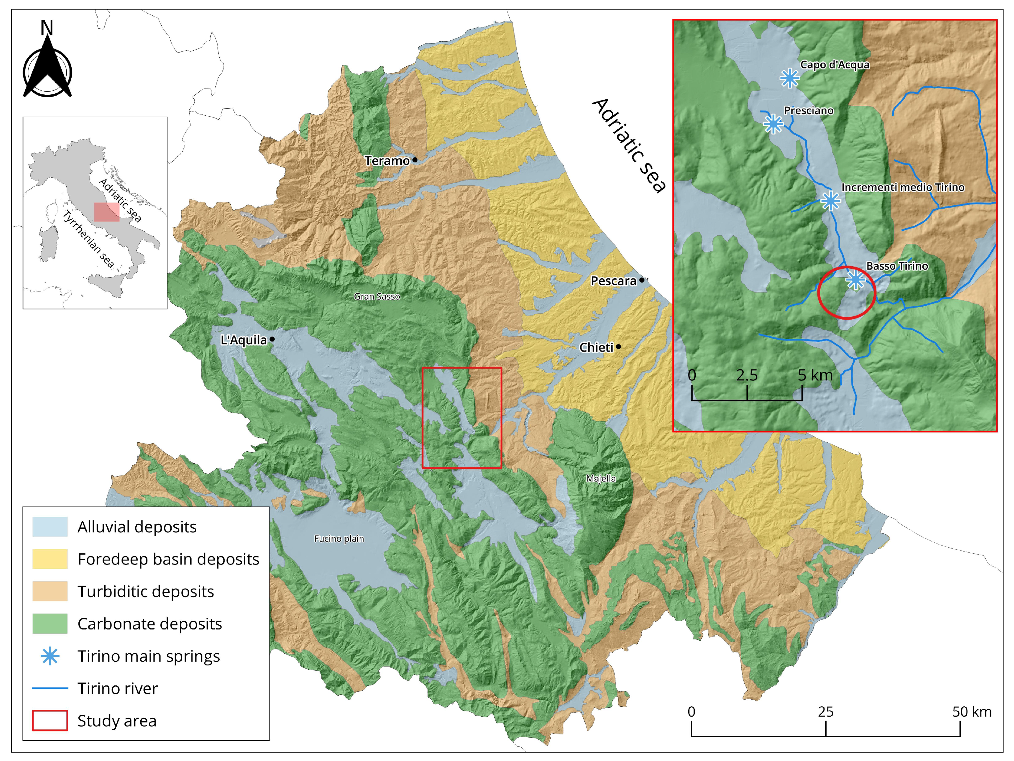
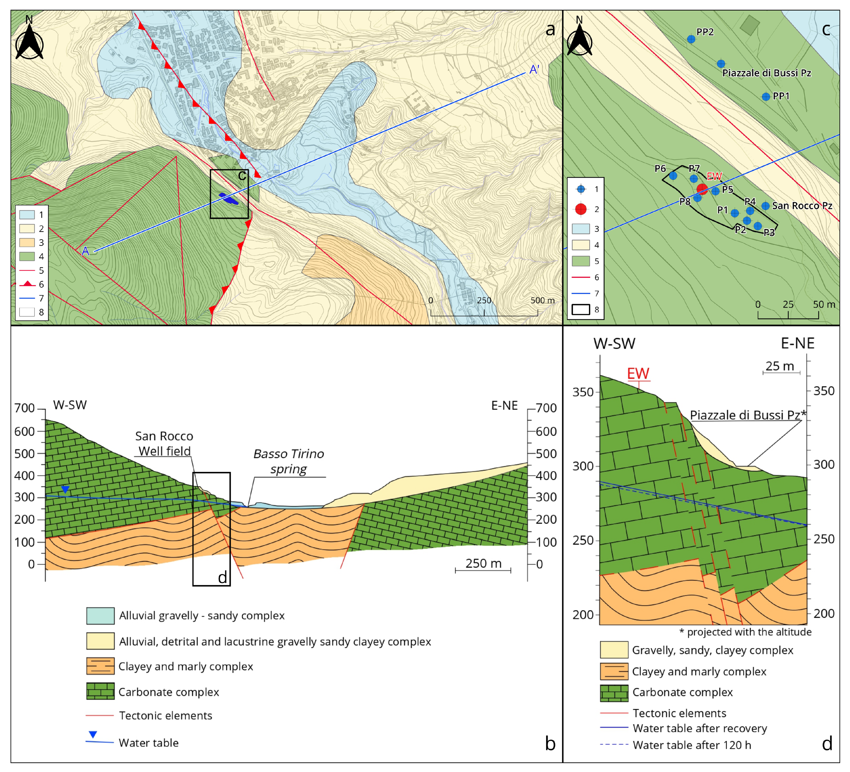
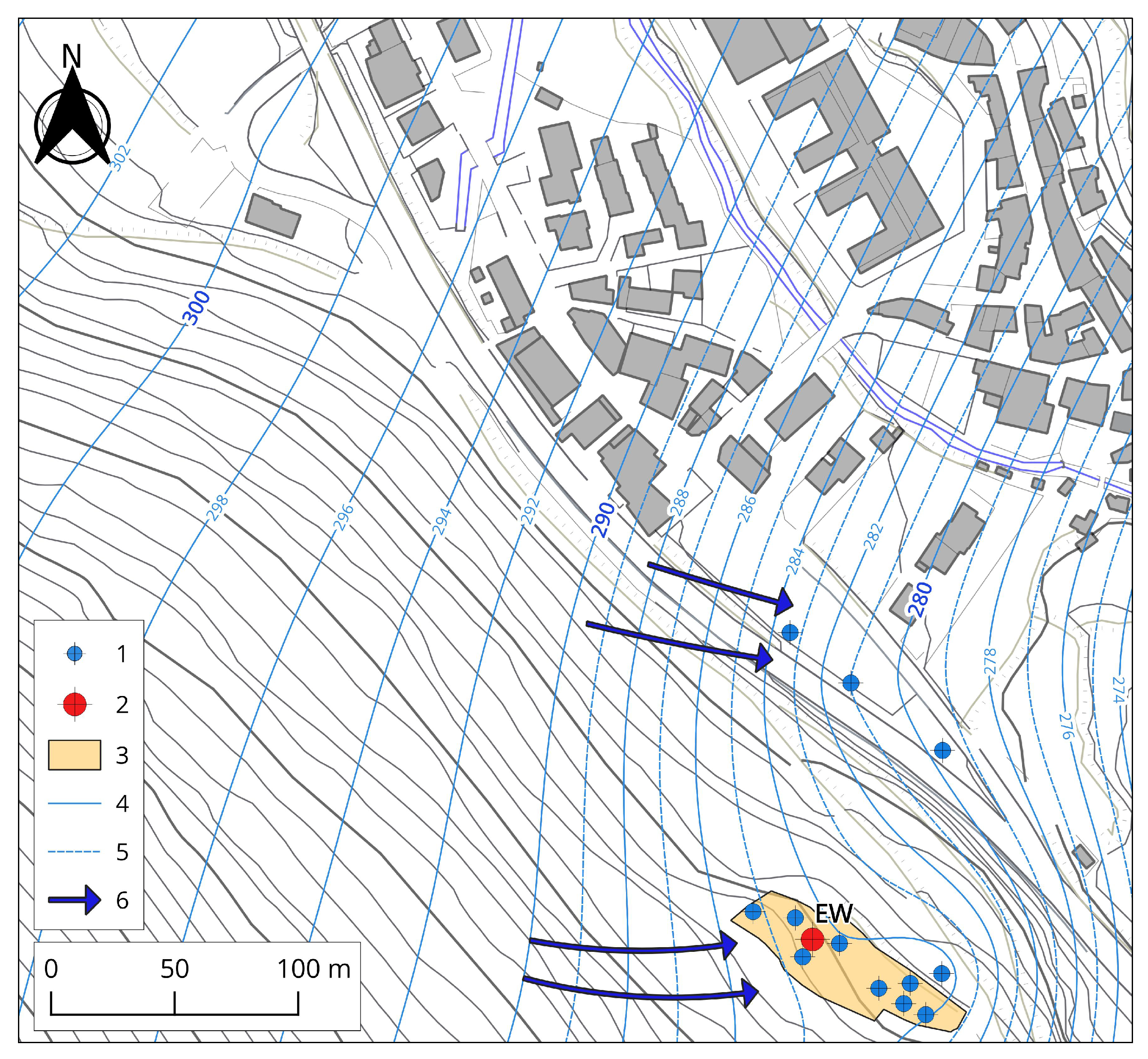
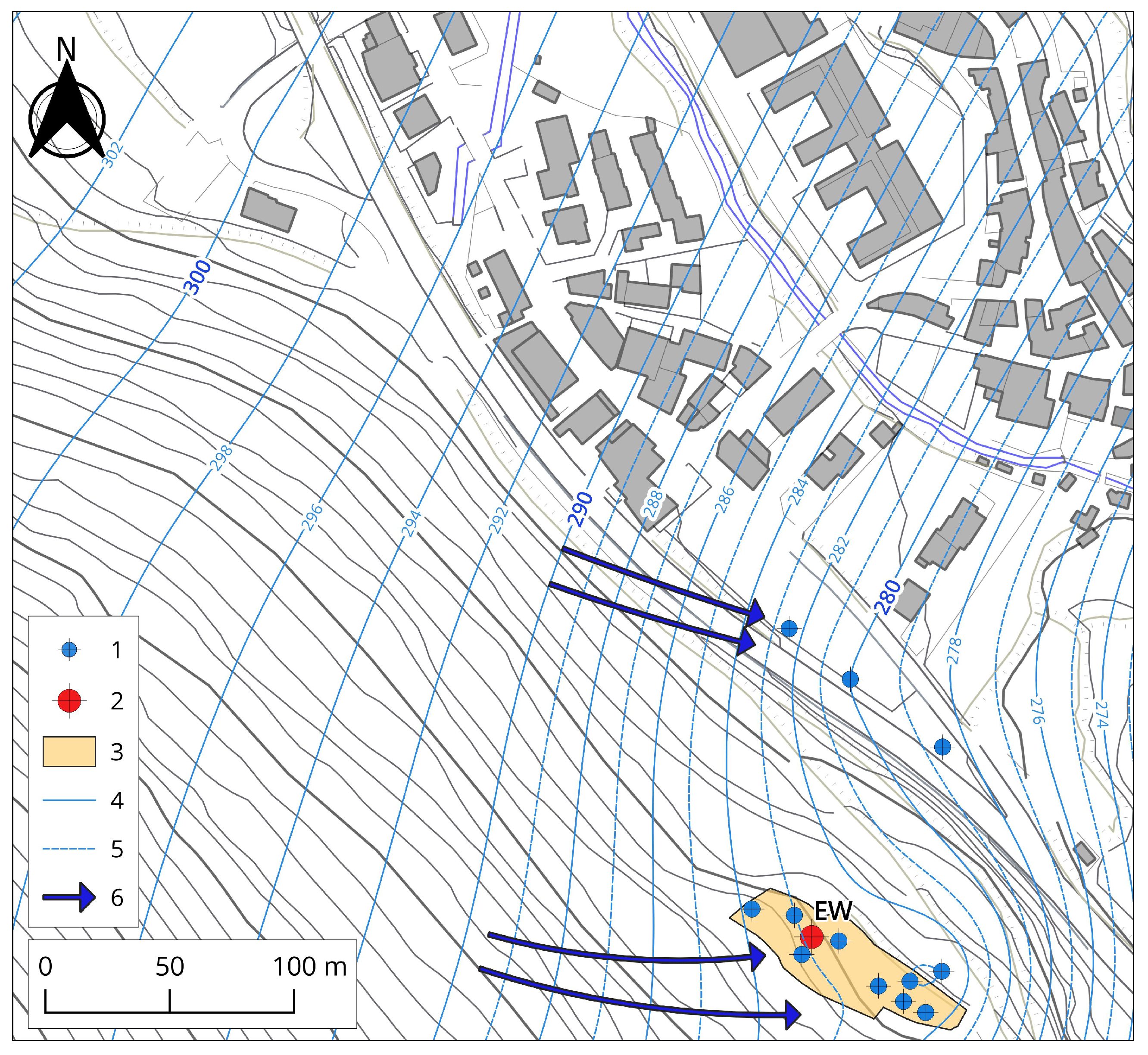
2.1. Site Description

The study site is located at the foot of the Apennines chain, in the Abruzzo Region, inside the Tirino River valley (Figure 1), where the carbonate formations meet the marly–arenaceous foredeep deposits. In detail, in this area, a superposition between the Gran Sasso carbonate unit and the Morrone–Roccatagliata, through trust faults which involve the marly–arenaceous Laga Formation, can be observed. In this framework, the Tirino river valley was created by an extensional tectonic and filled by quaternary deposits, such as lacustrine, detrital, and strictly alluvial ones.

From the hydrogeological point of view, this area hosts the most important aquifers of the Abruzzo Region: the Gran Sasso aquifer, 700 km²-wide [5], and the Morrone aquifer [34]. As mentioned above, these units are mainly calcareous and then characterized by high hydraulic conductivity due to fracturing and karstification and with wide recharge areas. The quaternary deposits’ hydraulic conductivity changes according to the grain size, and consequently they allow water flow or create local aquicludes.

In the lowest areas, where the carbonate structures are in contact with the marly ones, these aquifers generate basal springs whose discharges are between 6 m³/s and 1 m³/s; thus, the Tirino is an almost exclusively spring-fed river with a length of 13 km and a streamflow between 12 and 18 m³/s [35]. The main springs are the Basso Tirino one (Q ~ 6 m³/s), the Capo d’Acqua springs group (Q ~ 3 m³/s), and the Presciano (Q ~ 2 m³/s) ones (Figure 1); furthermore, minor springs (Q ~ 1 m³/s) are also present and called Incrementi Medio Tirino [35].

According to the literature data [36] the total spring discharge of the area is 13 m³/s derived from the previous springs, and from riverbed increases from other sources.

Locally, the geological and hydrogeological framework is quite complex because of the heterogeneity of the deposits; Figure 2 shows the detailed hydrogeological set-up of the study area, from the literature data and available borehole stratigraphies [37,38,39,40]. The Gran Sasso carbonate complex is in contact with the marly–clayey one, creating a no-flux hydrogeological limit.

2.2. Well Field Set-Up

The San Rocco well field (Figure 2) is on the left side of the Tirino river, with eight wells and a piezometer (Pz) which draw water for drinking purposes; the global pumping rate varies through seasons depending on the request and on the availability of other water sources such as springs. The pumping rate is usually between 550 and 750 L/s, except during spring (April and May), where it is 200 L/s. A smaller well field (Piazzale di Bussi), located close to the San Rocco one, is used to integrate water requests during late summer and fall, with a 100 L/s pumping rate.

For monitoring reasons, a piezometer 1 km away from the field was also considered for the Cartignano one.

The eight San Rocco wells were approximated to a single well called the equivalent well (EW), and to define its position, the single pumping rates and the locations of all the San Rocco wells have been considered (Figure 2).

2.3. Step-Drawdown Test

Usually, pumping tests are not suitable for carbonate aquifers like this, where hydraulic conductivity is due to fracturing and karstification; however, a step-drawdown test has been performed and the equivalent hydraulic parameters have been estimated considering the carbonate aquifer as a porous one, as well as the influence radius, when the pumping rate was at maximum.

The step-drawdown test was described by Jacob [41], to observe the drawdown in a well while the pumping rate is increased by step [42]; in each step, the discharge rate is kept constant, and it is increased when the steady state is reached.

The step-drawdown test schedule for this study is shown in

Table 1. Pumping test schedule.

Step	Period	Pumping Rate (L/s)	Working Wells	Monitoring Wells
T0		635
Recovery	2.00	0	–	P5—P6—Pz San Rocco–Pz Piazzale–Pz Cartignano
1	22.45	453	P1—P2—P3—P7—P8	P5—P6—Pz San Rocco–Pz Piazzale–Pz Cartignano
2a	7.55	522	P1—P2—P3—P4—P7—P8	P5—P6—Pz San Rocco–Pz Piazzale–Pz Cartignano
2b	16.20	560	P1—P3—P4—P5—P7—P8	P5—P6—Pz San Rocco–Pz Piazzale–Pz Cartignano
3	72.55	740	P1—P2—P3—P4—P5—P6—P7—P8	P5—P6—Pz San Rocco–Pz Piazzale–Pz Cartignano

and organized to avoid the interruption of the drinking service.

As can be seen, the water distribution was turned off for only 2 h for the recovery step, and to obtain the so-called “initial steady state”, for each step an increasing number of wells was switched on, keeping the monitoring wells and piezometers fixed; each step lasted at least 24 h.

After the step-drawdown ended, the water level had been monitored for 114 days from the beginning of the third step; this allowed summer period monitoring when the pumping rate was the same as in the third step (740 L/s). Only a small adjustment in drawdown was recorded, probably due to the switching on and switching off of the Piazzale di Bussi well field with a pumping rate of 100 L/s.

2.4. Data Elaboration

Considering the available atypical data and the derived approximations, two of the simplest consolidated methods were chosen for data elaboration.

For the steady state, the Dupuit method was used, while for the unsteady state, the Theis one was used; both approaches allowed the hydraulic conductivity and influence radius estimation.

The Dupuit theory [43] considers the radial flow in a well pumping at a constant rate (Q) and the spreading of a depression cone until a certain distance (influence radius) at which the drawdown is null because of the equilibrium between pumping and aquifer response.

Some conditions must be present, such as steady-state conditions, which mean that in each point of the aquifer the velocity vector must be constant in time, the aquifer must be homogeneous and isotropic, Darcy’s law [44] must be valid, the flow has to be horizontal, and the same velocity in a vertical section is needed. This method can be applied to both phreatic and confined aquifers and in this specific case, the aquifer was considered to be phreatic (Figure 3).

The Dupuit equation is

$$Q=1.366K\frac{{h_0}^2-{h_w}^2}{\ln r_0/r_w}$$

(1)

where Q is the pumping rate (m³/s), r₀ is the distance between the pumping well and the no drawdown point, r_w is the pumping well radius, and h₀ and h_w are the saturated thickness in the static condition and the saturated thickness in the pumping well, respectively.

If two observation wells are considered, the Dupuit–Thiem equation [45] can be applied:

$$Q=1.366K\frac{{h_2}^2-{h_1}^2}{\ln r_2/r_1}$$

(2)

consequently, the equation for the hydraulic conductivity (K) estimation is

$$K=\left(\frac{Q}{1.366}\right)\mathit{log}\frac{r_2}{r_1}/\left({h_2}^2-{h_1}^2\right)$$

(3)

where Q is the pumping rate (m³/s), r₁ is the distance between the observation well P1 and the pumping well, r₂ is the distance between the observation well P2 and the pumping well, and h₁ and h₂ are the saturated thickness in observation wells P1 and P2 with static conditions, respectively (Figure 3).

The estimation of the influence radius (r₀) was carried out using two equations, the Dupuit [43] and the Sichardt [46] ones.

The Dupuit equation is

$$\ln r_0=\left(\frac{\left({h_0}^2-{h_1}^2\right)}{\left({h_2}^2-{h_1}^2\right)}\left(\ln \frac{r_2}{r_1}\right)\right)+\ln r_1$$

(4)

while the Sichardt equation is

$$r_0=3000\left(h_0-h_w\right)\sqrt{K}$$

(5)

where r₁ is the distance between an observation well P1 and the pumping well, such as r₂, h₀ is the water table depth in static condition, h_w is the hydraulic head in the pumping well, and h₁ and h₂ are the hydraulic heads in the observation wells P1 and P2 with static conditions, respectively.

Taking into account the thickness of the aquifer, transmissivity (T) can be also estimated, using

$$T=Kb$$

(6)

where K is the hydraulic conductivity and b the aquifer thickness.

In this study, for data elaboration, the abovementioned equivalent well (EW) was considered a pumping well, and P5 and P6 wells, Cartignano, Piazzale di Bussi, and San Rocco piezometers were considered to be monitoring wells.

The unsteady theory by Thies [11] is based on the principle that if pumping continues, a wider portion of the aquifer is involved in it; as a consequence, there is not a fixed influence radius, but it becomes bigger, as does the depression cone.

Considering the large aquifer extension [5] and the low drawdown compared with the aquifer thickness, in this case, the carbonate aquifer was considered to be confined and the Theis equation was applied,

$$h_0-h=\frac{Q}{4\pi T}\underset{0}{\overset{\infty }{\int }}\frac{e^{-u}du}{u}$$

(7)

where $u=\frac{r^2}{4Tt}$ and $\underset{0}{\overset{\infty }{\int }}\frac{e^{-u}du}{u}=W\left(u\right)$ were called Well function, h₀ is the hydraulic head at a distance r from the well, h is the hydraulic head after a certain time t, Q is the pumping rate (m³/s), T is the transmissivity, and S is the storage coefficient.

This method can be applied if the aquifer is homogeneous and isotropic, it is confined by a constant thickness, and the well goes through the aquifer’s thickness with an infinitesimal diameter [47].

Equation (7) can be solved using the Jacob–Cooper approximation [12] and it becomes

$$h_0-h=\mathsf{\Delta }h=\frac{0.183Q}{T}\left(\log \left(\frac{2.25Tt}{r^{2}S}\right)\right)$$

(8)

where $\frac{0.183Q}{T}=C$ and is the angular coefficient of the line “Drawdown vs. Log time”.

2.5. Hydrochemical Parameters

Temperature (T), pH, electrical conductivity (χ), and redox potential (Eh) were monitored with a portable multiparameter probe during the pumping tests in order to identify any variation in physico-chemical features due to the expansion of the cone or involved portions of aquifer with different lithological characteristics and consequently different water–rock interactions. These parameters have been measured in P2.

2.6. Consideration about the Atypicality of the Test

• This test has been defined as atypical because of the use of some approximations:
• The well field was pumping water during the test;
• The pumping rate was increased using a higher number of pumping wells instead of raising a single one;
• The pumping rate for each step was decided by the managing organization based on the features of the available pumps;
• This method was applied to a carbonate aquifer that was considered like a porous one;
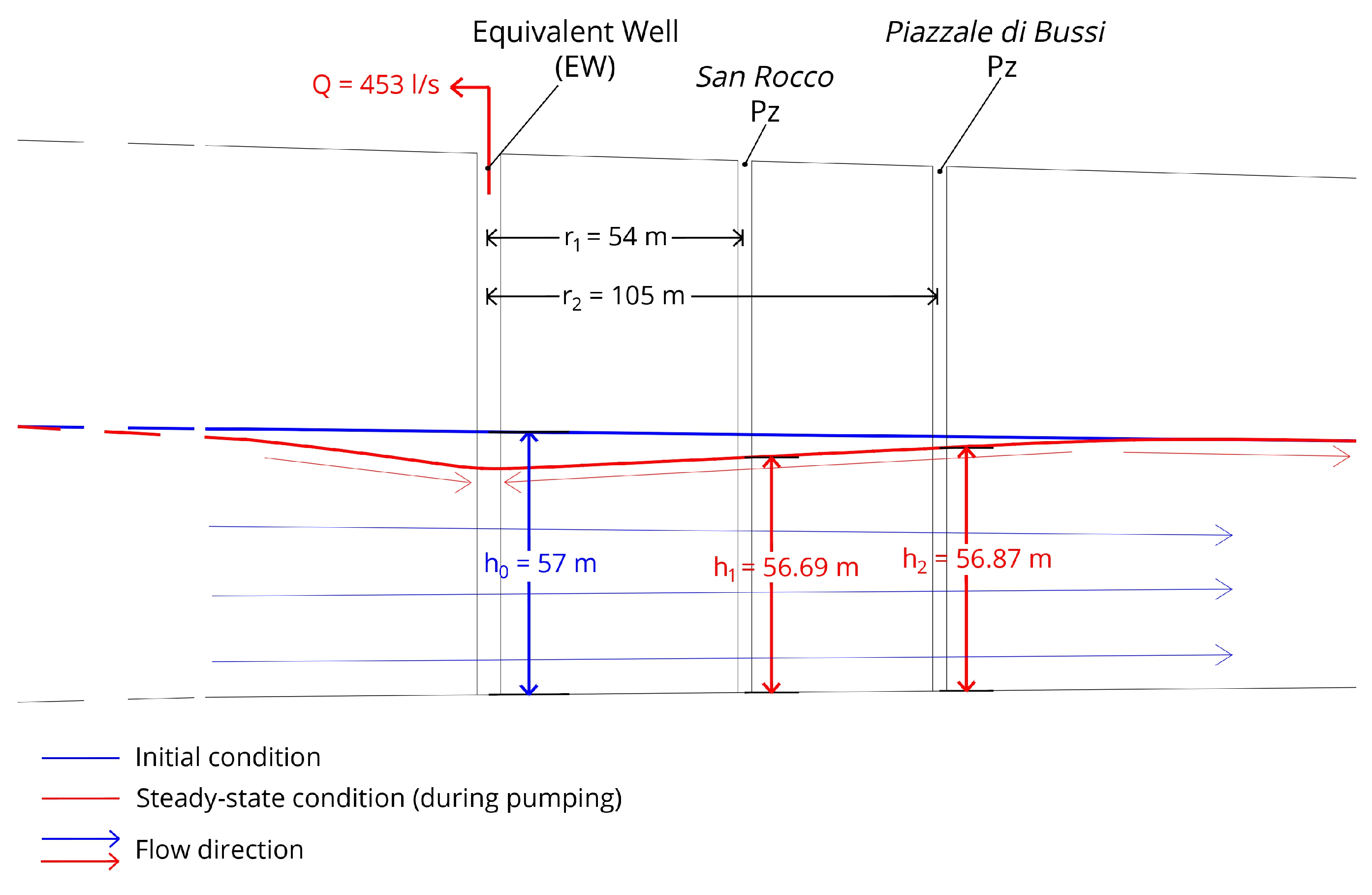
• The conceptual model (Figure 3) was simplified compared to the reality;
• The data elaborations were executed using an equivalent well, instead of a single one.

3. Results

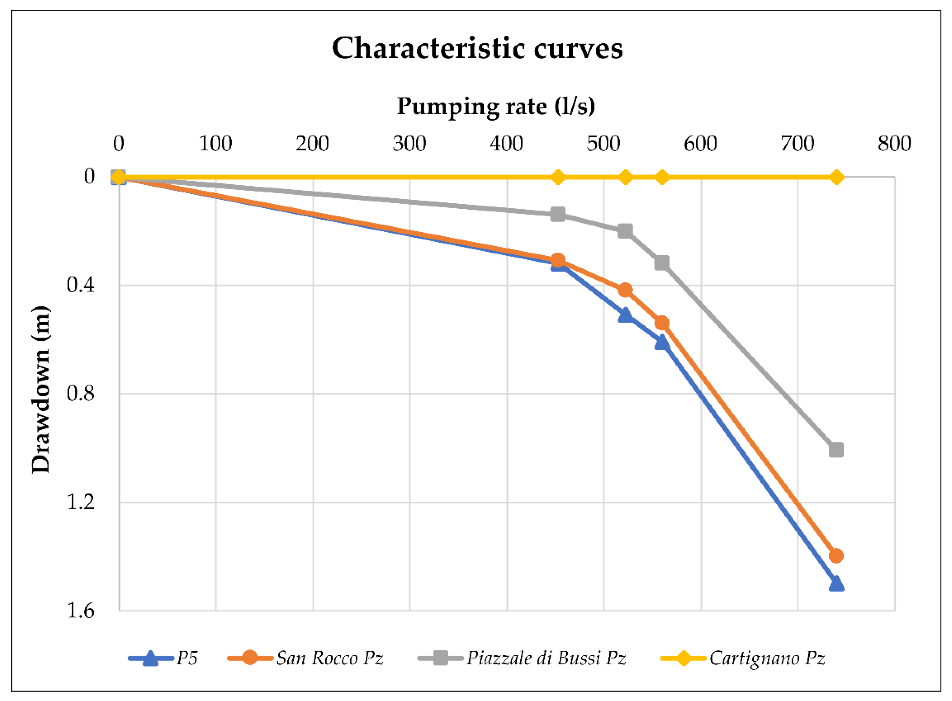
3.1. Step-Drawdown Test, Steady-State Condition

During the execution of the step-drawdown test, P5 and P6 wells and San Rocco, Piazzale, and Cartignano piezometers were monitored (Figure 4 and

Table 2. Step-drawdown test results.

Well/Piez.	Step	Pumping Rate (L/s)	Distance from EW (m)	h1 (m)	h2 (m)	Δh (m)	ΔhTOT (m)
P5	Recovery	0	11	57.51	57.00	−0.51	-
	1	453	11	57.00	56.68	0.32	0.32
	2a	522	11	56.68	56.57	0.19	0.51
	2b	560	11	56.57	56.39	0.10	0.61
	3	740	11	56.39	55.50	0.89	1.50
P6	Recovery	0	27	57.72	57.00	−0.72	-
	1	453	27	57.00	56.88	0.12	0.12
	2a	522	27	56.88	56.82	0.06	0.18
	2b	560	27	56.82	56.71	0.11	0.29
	3	740	27	56.71	49.17	7.54	7.83
San Rocco Pz	Recovery	0	54	57.87	57.00	−0.87	-
	1	453	54	57.00	56.69	0.31	0.31
	2a	522	54	56.69	56.58	0.11	0.42
	2b	560	54	56.58	56.46	0.12	0.54
	3	740	54	56.46	55.60	0.86	1.40
Piazzale di Bussi Pz	Recovery	0	105	57.55	57.00	−0.55	-
	1	453	105	57.00	56.86	0.14	0.14
	2a	522	105	56.86	56.80	0.06	0.20
	2b	560	105	56.80	56.68	0.12	0.32
	3	740	105	56.68	55.99	0.69	1.01
Cartignano Pz	Recovery	0	1158	57.01	57.00	−0.01	-
	1	453	1158	57.00	57.00	0.00	-
	2a	522	1158	57.00	57.00	0.00	-
	2b	560	1158	57.00	57.00	0.00	-
	3	740	1158	57.00	57.00	0.00	-

); the geometry of the aquifer was simplified and, in static condition, a 57 m saturated thickness was considered. Moreover, the unstoppable water supply and the use of the well field pumps for the test did not allow the execution of the “typical steps” for the step-drawdown test; indeed, in this case, the pumping rates were decided on the basis of the single pumping rate of each pump. In Table 2, the pumping rates of each step can be observed; step 2 was divided into two sub-steps because of the working well field.

In

Table 3. Hydraulic conductivity and transmissivity estimation (Pz stands for piezometer).

		Monitoring Well Pairs
		P5 –Piazzale Pz	San Rocco Pz– Piazzale Pz
Step	Pumping Rate (L/s)	K (m/s)	K (m/s)	T (m2/s)
1	453	0.0050	0.0050	0.285
2a	522	0.0044	0.0044	0.250
2b	560	-	0.0048	0.274
3	740	-	0.0036	0.205

, the hydraulic conductivity estimation is summarized; the P5–Piazzale piezometer and San Rocco–Piazzale piezometers were taken into account, and P5 was considered only when it was not working. Equations (3) and (6) were used for hydraulic conductivity and transmissivity estimation, respectively.

The mean hydraulic conductivity obtained was 4.5 × 10⁻³ m/s, while the mean transmissivity was 2.5 × 10⁻¹ m²/s considering an aquifer 57 m thick. Despite the issues faced during the test, the results showed a good convergence using different pumping rates (different steps) and different well/piezometer pairs.

The influence radius was calculated for each pumping rate, using piezometer data for the Dupuit equation [43] and P5 well data for the Sichard [46] one (

Table 4. Influence radius estimation.

Equation	Step	Pumping Rate (L/s)	h2 (Piazzale Pz) (m)	h1 (San Rocco Pz) (m)	r0 (m)
Dupuit	1	453	56.86	56.69	180
	2	560	56.68	56.46	280
	3	740	55.99	55.6	590
Equation	Step	Pumping Rate (L/s)	h0 (m)	hw (m)	r0 (m)
Sichard	1	453	57	56.70	64
	2	560		56.40	123
	3	740		55.50	302

).

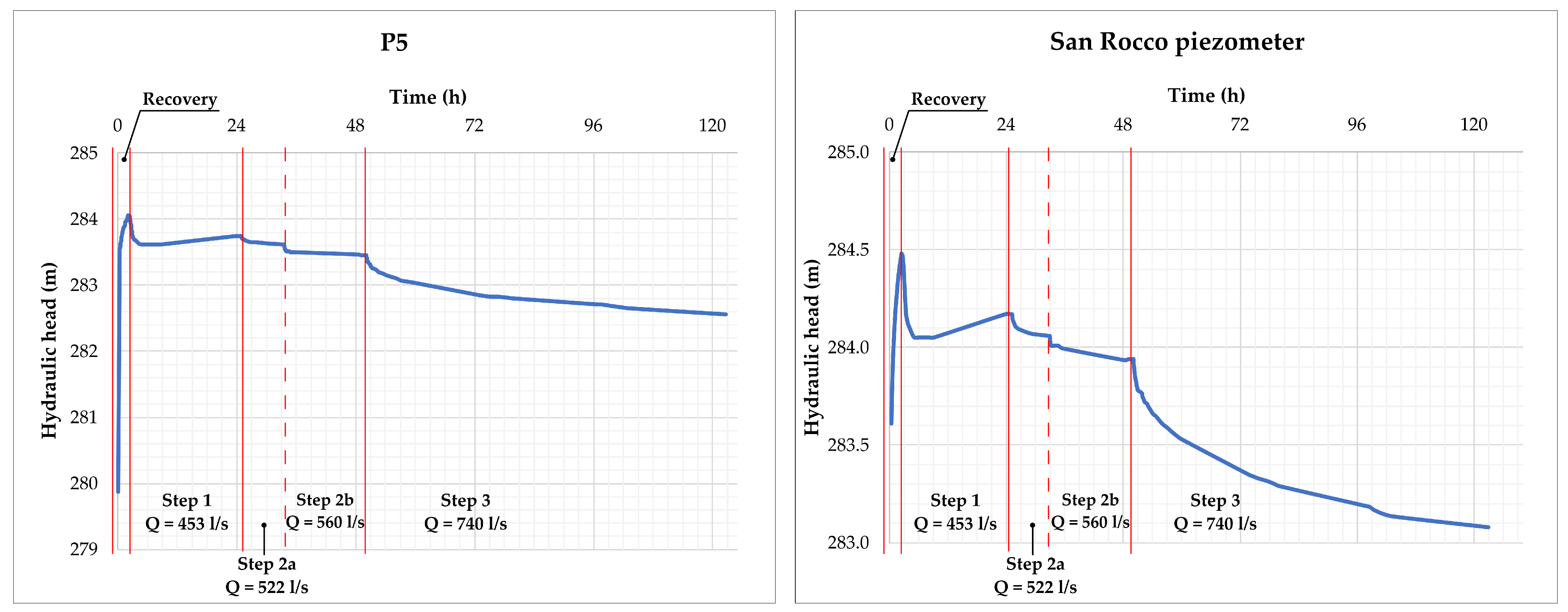
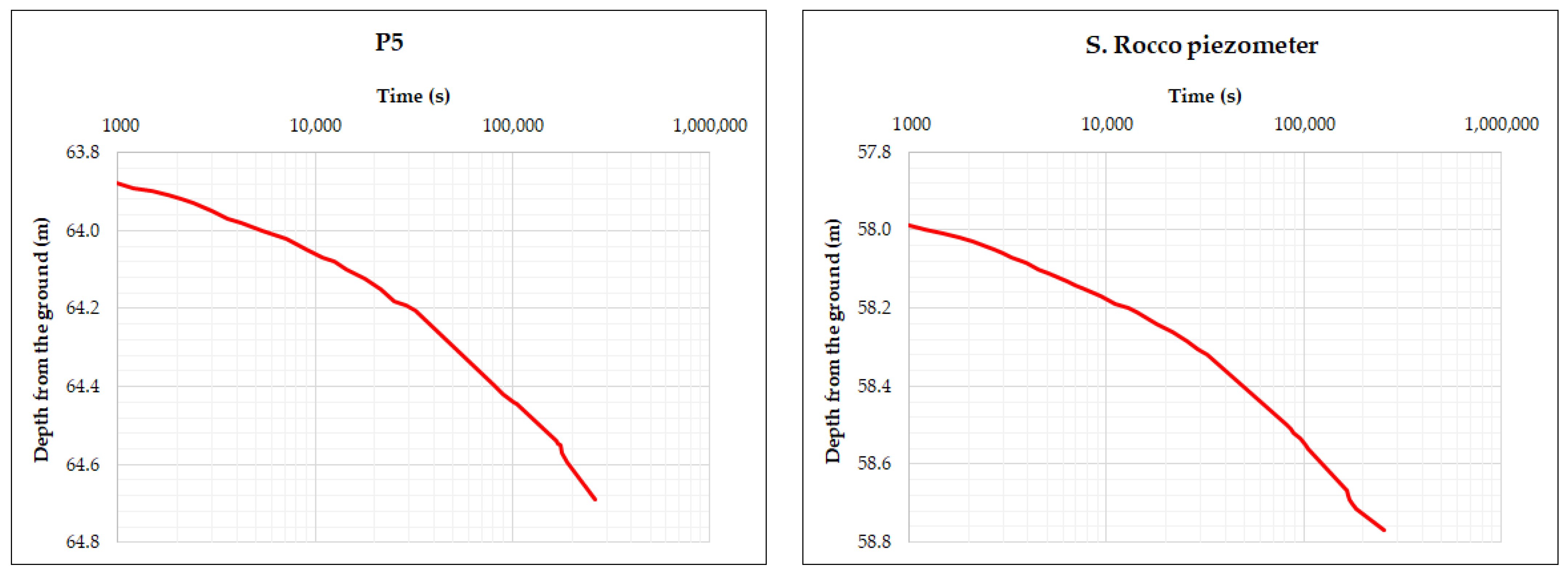
3.2. Step-Drawdown Test, Unsteady-State Condition

The unsteady-state elaboration was performed using P5 well and San Rocco and Piazzale piezometer data (Figure 5); as for the steady-state estimation, the geometry of the aquifer was considered to be 57 m thick. Transmissivity (T) was estimated from Equation (8), while hydraulic conductivity was taken from Equation (6).

The mean transmissivity obtained was 3.3 × 10⁻¹ m²/s, the mean hydraulic conductivity was 5.6 × 10⁻³ m/s, and the storage coefficient varied between 0.06 and 0.15 (

Table 5. Unsteady-state elaboration and results (for symbols see paragraph on “Data elaboration”).

Well/Piez.	Step	Q (L/s)	C	t0 (s)	T (m2/s)	K (m/s)	S
P5	1	453	0.42		0.20	0.003
	3 I log cycle	740	0.18		0.75	0.013
	3 II log cycle.	740	0.38		0.36	0.006
Pz San Rocco	1	453	0.39		0.21	0.004
	3 I log cycle	740	0.175	250	0.77	0.014	0.15
	3 II log cycle	740	0.36	1600	0.38	0.007	0.46
Pz Piazzale di Bussi	1	453	0.21		0.39	0.007
	3 I log cycle	740	0.14	280	0.97	0.017	0.06
	3 II log cycle	740	0.32	2200	0.42	0.007	0.19

).

The results obtained from the test elaborated using the unsteady state did not show good convergence among themselves like the steady-state ones. In any case, the mean value obtained from the different elaborations, estimated using different log-cycles and piezometers, was perfectly comparable with that obtained from the steady-state calculations.

3.3. Long-Term Observations

In

Table 6. Long-term observations in dynamic conditions.

Well/Piezometer	Distance from EW	Head (Steady-State Cond.)	Drawdown * (After 5 Days)	Drawdown * (After 114 Days)
P5	11 m	284.06	−2.0 m	−1.3 m
P6	26.5 m	284.81	−7.8 m	−8.7 m
Pz San Rocco	54 m	284.48	−1.4 m	−1.3 m
Pz Piazzale di Bussi	105 m	280.93	−1.0 m	−1.2 m

Note: * compared with static level.

, the drawdowns observed after 114 days are summarized; as can be seen in P5, San Rocco, and Piazzale di Bussi piezometers, the drawdown has slight differences. P6 is an exception because a difference in the meter was observed, which was because of the superposition effect during the use of both well fields during the summer season.

3.4. Hydrochemical Parameters

Looking at

Table 7. Monitored physico-chemical parameters.

Time from Test Beginning (hour·min)	T (°C)	χ (µS/cm)	pH	Eh (mV)
7.00	12.2	583	8.3	126
24.15	11.7	580	8.2	155
25.50	11.8	573	8.0	173
27.00	11.8	573	8.2	144
29.05	11.8	573	8.1	194
34.50	11.6	579	8.1	155
47.40	11.7	578	8.2	147
50.30	11.8	574	8.1	213
52.40	11.9	574	8.2	223
56.45	11.7	572	8.2	160
72.05	11.8	576	8.2	178
76.00	11.9	577	8.2	216
78.35	12.0	577	8.1	189
95.45	11.7	535	8.0	164

, a constant trend can be observed; indeed, during the pumping test, no parameters had significant variations except for the redox potential, which had values between 126 mV and 223 mV because of the oxygenation due to water exploitation.

This trend indicates a homogenous aquifer from a rock–water interaction point of view, and the aquifer portion involved in pumping did not interfere with physico-chemical parameters.

The mean temperature value was 11.8 °C, the mean electrical conductivity was 575 µS/cm, and the mean pH was 8.1.

4. Discussion

4.1. Step-Drawdown Test, Steady-State Condition

The step-drawdown test results can be analyzed in detail using both a hydraulic head vs. time plot (Figure 4) and the characteristic curves (Figure 6). In the first case, as can be seen in Figure 4, a very fast recovery in well P5 was recorded; this was because of an anomalous response of the well system to pumping: the well casing empties quickly and is not compensated by the aquifer, so when recovery starts filling is fast inside the well casing with a 3.8 m rise in P5.

Figure 6 shows the characteristic curve of each monitored well or piezometer, where drawdown vs. pumping rate is plotted; as can be seen, drawdown decreases away from the well field, the curves are parallel to each other despite their distance from the well field, and the Cartignano piezometer, located at over 1 km from the well field, is not affected by drawdown; these observations imply that the tested aquifer has homogeneous behavior.

The water table reconstruction (Figure 7) indicates a west–east flow direction in the San Rocco well field and a north-west/south-east one in the Piazzale di Bussi well field; the hydraulic gradient is 0.02, increasing from the north-west to the south-east.

4.2. Step-Drawdown Test, Unsteady-State Condition

Looking at Figure 5, the plot “depth from the ground vs. time” is not a straight line. This because of the unconventional type of test; to carry out the transmissivity, the straighter portions of the plots were considered. The potentiometric map at the end of the third step, 120 h after the test beginning, is in Figure 8, and demonstrates the same flow directions of the static conditions.

The water table decrease was restricted to the well fields area, with a 1.4 m drawdown in the San Rocco well field and 1.0 m in the Piazzale di Bussi one when the pumping rate was at maximum (Q = 740 L/s); the hydraulic gradient was 0.026, increasing from north-west to south-east.

5. Conclusions

An atypical step-drawdown test in a carbonate aquifer was performed using an increasing number of pumping wells to reach the maximum available pumping rate, without turning off the water supply.

The hydrodynamic parameters were measured using both steady-state and unsteady-state equations; the obtained results showed a substantial convergence between both methods. In the first case, the mean hydraulic conductivity was 4.4 × 10⁻³ m/s and the mean transmissivity, with an aquifer thickness of 57 m, was 2.5 × 10⁻¹ m²/s. In the unsteady-state condition, the mean hydraulic conductivity was 5.6 × 10⁻³ m/s, the mean transmissivity was 3.3 × 10⁻¹ m²/s, and the storage coefficient ranged from 0.06 to 0.15. The influence radius, calculated using the equivalent well, varied from 300 to 590 m when the pumping rate was at maximum.

Data elaboration using the characteristic curves (Figure 6) highlighted the homogeneous behavior of the flow field and homogeneous aquifer hydrodynamic parameters confirmed by the physico-chemical monitoring during the pumping test; the hydrochemical parameters were constant throughout the test, with mean values of 11.8 °C for temperature, 575 µS/cm for electrical conductivity, and 8.1 for pH.

The maximum drawdown, equal to 1.4 m, was reached after 120 h from the test beginning and after 72 h from the application of the maximum pumping rate (740 L/s); the drawdown after 114 days was very similar to the measured during the test, with slight differences when the Piazzale di Bussi well fields had been switched on.

These results show the high potentialities of this carbonate aquifer, highlighting limited drawdown when the pumping rate is at maximum, even after 3 months of pumping. In addition, the results have confirmed the possibility of executing this atypical test in a similar context, especially when the well field work is subject to aqueduct requests.

In conclusion, the pumping test led to coherent results for hydrodynamic parameters despite the use of this method in atypical manner, using pumping wells for water exploitation for both the monitoring and execution of the test.

References

1. Lemieux, J.M.; Therrien, R.; Kirkwood, D. Small scale study of groundwater flow in a fractured carbonate-rock aquifer at the St-Eustache quarry, Québec, Canada. Hydrogeol. J. 2006, 14, 603–612. [Google Scholar] [CrossRef]
2. Boni, C.; Bono, P.; Capelli, G. Schema Idrogeologico dell’Italia Centrale. Mem. Soc. Geol. Ital. 1986, 35, 991–1012. [Google Scholar]
3. Cassa per il Mezzogiorno; Celico, P. Idrogeologia dei massicci carbonatici, delle piane quaternarie e delle aree vulcaniche dell’Italia centro-meridionale. In Quaderni della Cassa per il Mezzogiorno; Cassa per il Mezzogiorno: Rome, Italy, 1983; Volume 4. [Google Scholar]
4. Celico, P. Considerazioni sull’idrogeologia di alcune zone dell’Italia centro-meridionale alla luce dei risultati di recenti indagini geognostiche. Mem. Note Ist. Geol. Appl. 1979, 15, 1–43. [Google Scholar]
5. Petitta, M.; Tallini, M. Idrodinamica sotterranea del massiccio del Gran Sasso (Abruzzo); nuove indagini idrologiche, idrogeologiche e idrochimiche (1994–2001). Boll. Soc. Geol. Ital. 2002, 121, 343–363. [Google Scholar]
6. Dragoni, W.; Sukhija, B.S. Climate Change and Groundwater: A Short Review. Geol. Society Spec. Pubbl. 2008, 288, 1–12. [Google Scholar] [CrossRef]
7. Green, T.R.; Taniguchi, M.; Kooi, H.; Gurdak, J.J.; Allen, D.M.; Hiscock, K.M.; Treidel, H.; Aureli, A. Beneath the surface of global change: Impacts of climate change on groundwater. J. Hydrol. 2011, 405, 532–560. [Google Scholar] [CrossRef]
8. Ndehedehe, C.E.; Adeyeri, O.E.; Onojeghuo, A.O.; Ferreira, V.G.; Kalu, I.; Okwuashi, O. Understanding global groundwater-climate interactions. Sci. Total Environ. 2023, 904, 166571. [Google Scholar] [CrossRef] [PubMed]
9. Lorenzi, V.; Sbarbati, C.; Banzato, F.; Lacchini, A.; Petitta, M. Recharge assessment of the Gran Sasso aquifer (Central Italy): Time-variable infiltration and influence of snow cover extension. J. Hydrol. Reg. Stud. 2022, 41, 101090. [Google Scholar] [CrossRef]
10. Petitta, M.; Banzato, F.; Lorenzi, V.; Matani, E.; Sbarbati, C. Determining recharge distribution in fractured carbonate aquifers in central Italy using environmental isotopes: Snowpack cover as an indicator for future availability of groundwater resources. Hydrogeol. J. 2022, 30, 1619–1636. [Google Scholar] [CrossRef]
11. Theis, C.V. The relation between the lowering of the piezometric surface and the rate and duration of discharge of a well using groundwater storage. Am. Geophys. Union Trans. 1935, 16, 519–524. [Google Scholar] [CrossRef]
12. Cooper, H.H., Jr.; Jacob, C.E. A generalized graphical method for evaluating formation constants and summarizing well field history. Am. Geophys. Union Trans. 1946, 27, 526–534. [Google Scholar] [CrossRef]
13. Chow, V.T. On the determination of transmissibility and storage coefficients from pumping test data. Trans. Am. Geophys. Union 1952, 33, 397–404. [Google Scholar] [CrossRef]
14. Jacob, C.E. Radial flow in a leaky artesian aquifer. Trans. Am. Geophys. Union 1946, 27, 198–208. [Google Scholar]
15. Hantush, M.S. Analysis of data from pumping tests in leaky aquifers. Trans. Am. Geophys. Union 1956, 37, 702–714. [Google Scholar] [CrossRef]
16. Boulton, N.S. Unsteady radial flow to a pumped well allowing for delayed yield from storage. Int. Assoc. Sci. Hydrol. Publ. 1954, 2, 472–477. [Google Scholar]
17. Boulton, N.S. Analysis of data from non-equilibrium pumping tests allowing for delayed yield from storage. Proc. Inst. Civ. Eng. 1963, 26, 469–482. [Google Scholar] [CrossRef]
18. Prickett, T.A. Type-curve solution to aquifer tests under water table conditions. Groundwater 1965, 3, 5–14. [Google Scholar] [CrossRef]
19. Neuman, S.P. Theory of flow in unconfined aquifers considering delayed response of the water table. Water Resour. Res. 1972, 8, 1031–1045. [Google Scholar] [CrossRef]
20. Neuman, S.P. Effect of partial penetration on flow in unconfined aquifers considering delayed gravity response. Water Resour. Res. 1974, 10, 303–312. [Google Scholar] [CrossRef]
21. Moench, A.F. Combining the Neuman and Boulton models for flow to a well in an unconfined aquifer. Groundwater 1995, 33, 378–384. [Google Scholar] [CrossRef]
22. Samani, S.; Vadiati, M.; Azizi, F.; Zamani, E.; Kisi, O. Groundwater level simulation using soft computing methods with emphasis on major meteorological components. Water Resour. Manag. 2022, 36, 3627–3647. [Google Scholar] [CrossRef]
23. Samani, S.; Vadiati, M.; Nejatijahromi, Z.; Etebari, B.; Kisi, O. Groundwater level response identification by hybrid wavelet–machine learning conjunction models using meteorological data. Environ. Sci. Pollut. Res. 2023, 30, 22863–22884. [Google Scholar] [CrossRef] [PubMed]
24. Lin, G.F.; Chen, G.R. An improved neural network approach to the determination of aquifer parameters. J. Hydrol. 2006, 316, 281–289. [Google Scholar] [CrossRef]
25. Vadiati, M.; Rajabi Yami, Z.; Eskandari, E.; Nakhaei, M.; Kisi, O. Application of artificial intelligence models for prediction of groundwater level fluctuations: Case study (Tehran-Karaj alluvial aquifer). Environ. Monit. Assess. 2022, 194, 619. [Google Scholar] [CrossRef] [PubMed]
26. Ayvaz, M.T. Simultaneous determination of aquifer parameters and zone structures with fuzzy c-means clustering and meta-heuristic harmony search algorithm. Adv. Water Resour. 2007, 30, 2326–2338. [Google Scholar] [CrossRef]
27. Tayfur, G.; Nadiri, A.A.; Moghaddam, A.A. Supervised intelligent committee machine method for hydraulic conductivity estimation. Water Resour. Manag. 2014, 28, 1173–1184. [Google Scholar] [CrossRef]
28. Prasad, K.L.; Rastogi, A.K. Estimating net aquifer recharge and zonal hydraulic conductivity values for Mahi Right Bank Canal project area, India by genetic algorithm. J. Hydrol. 2001, 243, 149–161. [Google Scholar] [CrossRef]
29. Samuel, M.P.; Jha, M.K. Estimation of aquifer parameters from pumping test data by genetic algorithm optimization technique. J. Irrig. Drain Eng. 2003, 129, 348–359. [Google Scholar] [CrossRef]
30. Ha, D.; Zheng, G.; Zhou, H.; Zeng, C.; Zhang, H. Estimation of hydraulic parameters from pumping tests in a multiaquifer system. Undergr. Space 2020, 5, 210–222. [Google Scholar] [CrossRef]
31. Tadj, W.; Chettih, M.; Mouattah, K. A new hybrid algorithm for estimating confined and leaky aquifers parameters from transient time-drawdown data. Soft Comput. 2021, 25, 15463–15476. [Google Scholar] [CrossRef]
32. Dashti, Z.; Nakhaei, M.; Vadiati, M.; Karami, G.H.; Kisi, O. A literature review on pumping test analysis (2000–2022). Environ. Sci. Pollut. Res. 2023, 30, 9184–9206. [Google Scholar] [CrossRef] [PubMed]
33. Tsoflias, G.P.; Halihan, T.; Sharp, J.M., Jr. Monitoring pumping test response in a fractured aquifer using ground-penetrating radar. Water Resour. Res. 2001, 37, 1221–1229. [Google Scholar] [CrossRef]
34. Conese, M.; Nanni, T.; Peila, C.; Rusi, S.; Salvati, R. Idrogeologia della Montagna del Morrone (Appennino abruzzese): Dati Preliminari. Mem. Soc. Geol. It. 2001, 56, 181–196. [Google Scholar]
35. Boni, C.; Pianelli, A.; Pierdominici, S.; Ruisi, M. Le grandi sorgenti del fiume Tirino (Abruzzo). Boll. Soc. Geol. Ital. 2002, 121, 411–431. [Google Scholar]
36. Regione Abruzzo, Servizio Acque e Demanio Idrico, Piano di Tutela delle Acque (PTA). Available online: https://www.regione.abruzzo.it/pianoTutelaacque/ (accessed on 21 February 2024).
37. Biava, F.; Consonni, M.; Francani, V.; Gattinoni, P.; Scesi, L. Delineation of Protection Zones for the Main Discharge Area of the Gran Sasso Aquifer (Central Italy) through an Integrated Geomorphological and Chronological Approach. J. Water Resour. Prot. 2014, 6, 1816–1832. [Google Scholar] [CrossRef]
38. Bigi, S.; Calamita, F.; Centamore, E. Carta Geologico-Strutturale dell’Area Compresa tra il Gran Sasso e il F. Pescara—Scala 1:50,000; Studio Faro: Rome, Italy, 1995. [Google Scholar]
39. APAT (Agenzia per la Protezione dell’Ambiente e per i Servizi Tecnici). Carta Geologica d’Italia in Scala 1:50,000, Foglio 360 “Torre de’ Passeri”; SEL.CA.: Florence, Italy, 2005. [Google Scholar]
40. APAT (Agenzia per la Protezione dell’Ambiente e per i Servizi Tecnici). Carta Geologica d’Italia in Scala 1:50,000, Foglio 369 “Sulmona”; SEL.CA.: Florence, Italy, 2005. [Google Scholar]
41. Jacob, C.E. Drawdown test to determine effective radius of artesian well. Trans. Am. Soc. Civ. Eng. 1947, 112, 1047–1070. [Google Scholar] [CrossRef]
42. Clark, L. The analysis and planning of step drawdown tests. Q. J. Eng. Geol. Hydrogeol. 1977, 10, 125–143. [Google Scholar] [CrossRef]
43. Dupuit, J. Mouvement de l’eau a travers le terrains permeables. C. R. Hebd. Seances Acad. Sci. 1857, 45, 92–96. [Google Scholar]
44. Darcy, H. Les Fontaines Publiques de la ville de Dijon; Dalmont: Paris, France, 1856. [Google Scholar]
45. Thiem, G. Hydrologische Methoden; J.M. Gebhardt: Leipzig, Germany, 1906. [Google Scholar]
46. Sichardt, W. Das Fassungsvermögen von Rohrbrunnen und Seine Bedeutung für die Grundwasserabsenkung, Insbesondere für Größere Absenkungstiefen; Springer: Berlin/Heidelberg, Germany, 1928. [Google Scholar]
47. Freeze, R.A.; Cherry, J.A. Groundwater; Prentice-Hall, Inc.: Englewood Cliff, NJ, USA, 1979. [Google Scholar]
Figure 1. Study area localization with regional and detailed hydro-geological framework.
Water 16 01047 g001
Figure 2. (a) Geo-hydrogeological map (simplified from APAT [39]): (1) gravelly–sandy complex; (2) gravelly–sandy and clayey complex; (3) clayey and marly complex; (4) Gran Sasso carbonate complex; (5) direct fault; (6) thrust; (7) cross-section trace; (8) well field area. (b) Hydrogeological cross-section. (c) Well field localization: (1) well; (2) equivalent well (EW); (3) gravelly–sandy complex; (4) gravelly–sandy and clayey complex; (4) Gran Sasso carbonate complex; (6) direct fault; (7) cross-section trace; (8) well field area. (d) Detailed hydrogeological cross-section.
Water 16 01047 g002
Figure 3. Pumping test scheme; the aquifer is approximated to a phreatic one in the steady state condition. Pz stands for piezometer. All parameters refer to Equations (2) and (3).
Water 16 01047 g003
Figure 4. Example of step-drawdown test plots: hydraulic head vs. time.
Water 16 01047 g004
Figure 5. Example of semilogarithmic plot “Depth from the ground vs. Time” for Q = 740 L/s (third step).
Water 16 01047 g005
Figure 6. Characteristic curves (drawdown vs. pumping rate) for the monitored wells and piezometers (Pz).
Water 16 01047 g006
Figure 7. Water table reconstruction in static conditions after recovery. (1) Well/piezometer; (2) equivalent well (EW); (3) well field area; (4) main contour; (5) auxiliary contour; (6) flow direction.
Water 16 01047 g007
Figure 8. Water table reconstruction in dynamic conditions after 5 days from the start of the test. (1) Well/piezometer; (2) equivalent well (EW); (3) well field area; (4) main contour; (5) auxiliary contour; (6) flow direction.
Water 16 01047 g008