Abstract
Understanding the subsurface is of prime importance for many geological and hydrogeological applications. Geophysical methods offer an economical alternative for investigating the subsurface compared to costly borehole investigations. However, geophysical results are commonly obtained through deterministic inversion of data whose solution is non-unique. Alternatively, stochastic inversions investigate the full uncertainty range of the obtained models, yet are computationally more expensive. In this research, we investigate the robustness of the recently introduced Bayesian evidential learning in one dimension (BEL1D) for the stochastic inversion of time-domain electromagnetic data (TDEM). First, we analyse the impact of the accuracy of the numerical forward solver on the posterior distribution, and derive a compromise between accuracy and computational time. We also introduce a threshold-rejection method based on the data misfit after the first iteration, circumventing the need for further BEL1D iterations. Moreover, we analyse the impact of the prior-model space on the results. We apply the new BEL1D with a threshold approach on field data collected in the Luy River catchment (Vietnam) to delineate saltwater intrusions. Our results show that the proper selection of time and space discretization is essential for limiting the computational cost while maintaining the accuracy of the posterior estimation. The selection of the prior distribution has a direct impact on fitting the observed data and is crucial for a realistic uncertainty quantification. The application of BEL1D for stochastic TDEM inversion is an efficient approach, as it allows us to estimate the uncertainty at a limited cost.
1. Introduction
Geophysical methods offer an economical alternative for investigating the subsurface compared to the use of direct methods. Most geophysical methods rely on a forward model to link the underlying physical properties (e.g., density, seismic velocity, or electrical conductivity) to the measured data and by solving an inverse problem. Deterministic inversions typically use a regularization approach to stabilize the inversion and resolve the non-unicity of the solution, yielding a single solution. However, uncertainty quantification is generally limited to linear noise propagation [1,2,3,4]. In contrast, stochastic inversion methods based on a Bayesian framework compute an ensemble of models fitting the data, based on the exploration of the prior model space [5]. Bayesian inversion is rooted in the fundamental principle that a posterior distribution can be derived from the product of the likelihood function and the prior distribution. Various strategies have been developed in this regard, as evidenced by the literature across several disciplines, including, but not limited to, hydrology and hydrogeology [6,7,8,9] or geophysics [10,11]. Although the increase in computer performance has advanced the use of stochastic approaches, long computational time remains an important issue for their broader adoption [12,13,14,15]. Indeed, most stochastic approaches rely on Markov chain Monte Carlo (McMC) methods for sampling the posterior model space [5], which require a large number of iterations and forward model computations.
Alternatives have been developed to estimate the posterior distribution at a limited cost such as Kalman ensemble generators [16,17] or Bayesian Evidential learning (BEL) [18,19]. BEL is a simulation-based prediction approach that has been initially proposed to by-pass the difficult calibration of subsurface reservoir models and to directly forecast targets from the data [20,21], with recent applications in geothermal energy [22,23,24], reservoir modelling [25,26,27,28], experimental design [29] and geotechnics [30]. It has also been quickly adopted by geophysicists to integrate geophysical data into model or properties prediction [24,31,32]. BEL has also been recently proposed as an efficient alternative for the 1D inversion of geophysical data (BEL1D) [18,19]. BEL1D circumvents the inversion process by using a machine learning approach derived from Monte Carlo sampling of the prior distribution. It has been proven efficient for the estimation of the posterior distribution of water content and relaxation time from nuclear magnetic resonance data [18], and the derivation of seismic velocity models from the analysis of the dispersion curve [19]. The main advantage of BEL1D is to rely on a smaller number of forward model runs than McMC approaches to derive the posterior distribution, leading to a reduced computational effort. Earlier work has shown that BEL1D converges towards the solution obtained from an McMC procedure but it slightly overestimates the uncertainty, especially in the case of large prior uncertainty [18]. The use of iterative prior resampling followed by a filtering of models based on their likelihood has been recently proposed to avoid uncertainty overestimation [19]. Although this increases the computational cost of BEL1D, it remains about one order of magnitude faster than McMC [19]. In this contribution, we propose to apply a threshold on the data misfit after the first BEL1D first iteration to circumvent the need for multiple iterations when prior uncertainty is large.
So far, BEL1D has only been applied to a limited number of geophysical methods. In this contribution, we apply the algorithm to the inversion of time-domain electromagnetic (TDEM) data. We combine BEL1D with the TDEM forward modelling capabilities of the open-source Python package SimPEG (version 0.14.1) [33,34] for the stochastic inversion of TDEM data. Electromagnetic surveys have proven to be efficient for delineating groundwater reservoir structure and water quality (e.g., [35,36,37]). In the last decades, the popularity of TDEM has largely increased with the adoption of airborne TDEM surveys for mineral but also hydrogeological applications (e.g., [38,39,40]). More recently, towed transient electromagnetic (tTEM) systems [41] and waterborne TDEM systems [42,43] were designed for continuous measurements of TDEM data, thus allowing to the coverage of large areas in relatively short times.
To date, the inversion of such extensive surveys relies on deterministic quasi-2D or -3D inversion [44], i.e., using a 1D forward model with lateral constraints. In the process of resolving inverse problems, which entails fitting observational data, the forward model representing the underlying physical processes is pivotal. However, this model is susceptible to errors inherent in the modelling process. The employment of an accurate numerical forward model imposes substantial computational demands, consequently constraining the feasible quantity of forward simulations [45].
In light of these computational constraints, it is a prevalent practice to resort to rapid approximation strategies for the forward solver [46,47], to work with a coarser discretization [48,49] or to deploy surrogate models to replace the expensive simulations [50,51,52].
Modelling errors may introduce significant biases in the posterior statistical analyses and may result in overly confident parameter estimations if these errors are not accounted for [52,53]. Hansen et al. [53] studied the effect of using approximate forward models on the inversion of GPR cross-hole travel time data and demonstrated that the modelling error could be more than one order of magnitude larger than the measurement error, leading to unwanted artifacts in the realizations from the posterior probability. For EM methods, studies have demonstrated the negative effect of using fast approximations of the forward model on the accuracy of the inversion [54,55,56]. In particular, for TDEM methods, using accurate models is computationally too expensive to be attractive for stochastic inversion of large data sets, as are those obtained from surveys with airborne or tTEM methods. Therefore, in this study we investigate a possible approach that balances accuracy in the modelling and reduced computational costs.
Stochastic approaches for the inversion of TDEM are therefore still uncommon (e.g., [13,15,56,57], yet these are computationally demanding for large data sets. Typically, the whole inversion needs to be re-run for every sounding, independently. Hence, developing a fast alternative is highly relevant for to-date hydro-geophysical investigations.
In this paper, we focus on the robustness of BEL1D to retrieve the posterior distributions of electrical subsurface model parameters from the inversion of TDEM data. The novelties of our contribution lie in the following:
- Demonstrating that BEL1D is an efficient approach for the stochastic inversion of TDEM data.
- Exploring the impact of the accuracy of the forward solver to estimate the posterior distribution, and finding a compromise between accuracy and computational cost.
- Proposing and validating a new thresholding approach to circumvent the need for iterations when the prior uncertainty is large.
- Applying the new approach to field TDEM data collected in the Luy River catchment in the Binh Thuan province (Vietnam) for saltwater intrusion characterization. This data set was selected because electrical resistivity tomography (ERT) data are available for comparison, but lack sensitivity at greater depth. The case study is also used to illustrate the impact of the selection of the prior on the posterior estimation.
The computational undertakings in this study are performed using the pyBEL1D package (version 1.1.0) [58] which serves as the computational backbone for our analyses. This integration of theoretical insights and practical applications is intended to advance the understanding and uncertainty quantification of TDEM surveys.
2. Materials and Methods
2.1. BEL1D
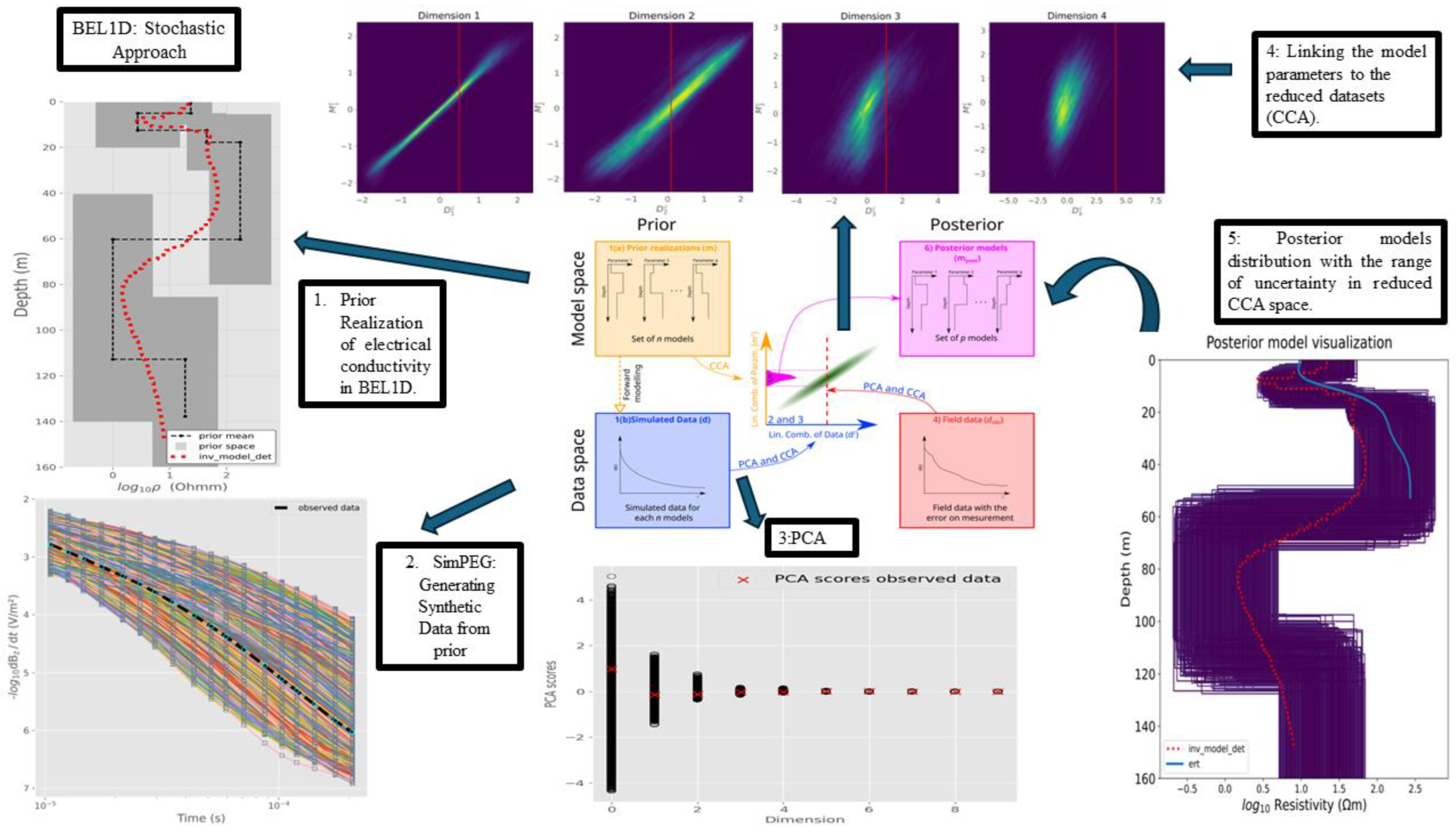
In contrast to deterministic approaches, BEL1D does not rely on the stabilization of the ill-posed inverse problem through regularization. Instead, BEL1D learns a statistical relationship between the target (the set of parameters of interest, in this case a subsurface layered model of the electrical conductivity) and the predictor (the geophysical data). This statistical relationship is derived from a combination of models and data (typically a few thousand) drawn from the prior distribution which reflects the prior geological knowledge. For each sampled model, the forward model is then run to generate the corresponding data set [18]. Next, a statistical relationship is learned in a lower dimensional space and used to calculate the posterior distribution corresponding to any data set consistent with the prior, without the need to run any new forward model. We refer to [18,19] for details about the algorithm. Here, we only provide a short overview. BEL1D consists of seven steps:
Step 1: Prior sampling and forward modelling
As in any stochastic inversion, the first step is to assign the range of prior uncertainty based on earlier field knowledge. For TDEM 1D inversion, we need to define the number of layers, their thickness and electrical conductivity. A set of prior models is sampled. For each sampled model, the corresponding TDEM data are simulated using the forward model. In this step, it is important to state the size of the transmitting and receiving loop and the waveform and magnetic momentum of the primary field, as well as the acquisition time and sampling of the decay-curve.
More specifically, this first step entails defining the prior model using a finite set of layers, with the final layer simulating the half-space. Except for this layer, which is defined by its conductivity only, the other layers are defined by their conductivity and thickness. Thus, the total number of model parameters or unknowns is . For each of those parameters, a prior distribution is described, which must reflect the prior understanding of the survey site. Such information can be based on either previous experiments or more general geological and geophysical considerations. Random models are sampled within the prior range, and the forward model is run for each one to calculate the corresponding noise-free data set (Figure 1, boxes 1 and 2):
where is the set of q model parameters and is the forward model solving the physics (see Section 2.2).
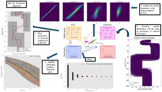
Figure 1.
The schematic diagram of BEL1D applied to TDEM data (modified from [18]).
Step 2: Reducing the dimensionality of data.
Lowering the dimensionality of the data is required to determine a statistical connection between the target and the predictor. Dimension reduction also helps to limit the impact of noise on the inversion [31]. Principal component analysis (PCA) identifies linear combinations of variables that explain most of the variability by using the eigenvalue decomposition [59]. Higher dimensions typically exhibit less variability and can be disregarded. Noise is propagated using Monte Carlo simulation [18,31] to estimate the uncertainties of the PCA scores caused by data noise (Figure 1 box 3). Similarly, the dimensions of model parameters q can be reduced if necessary.
Step 3: Statistical relationship between target (model parameters) and predictor (the reduced dataset)
Canonical correlation analysis (CCA) is used to determine a direct correlation between the target and predictor [18]. CCA essentially calculates the linear combinations of (reduced) predictor variables and target variables that maximize their correlation, producing a set of orthogonal bivariate relationships [59]. The correlation typically decreases with the dimensions, the first dimension being the most correlated (Figure 1 box 4).
Note that CCA is not the only approach for deriving a statistical relationship. Due to the expected non-linearity in the statistical relationship between seismic data and reservoir properties, [32] have used summary statistics extracted from unsupervised- and supervised-learning approaches including discrete wavelet transform and a deep neural network combined with approximated Bayesian computation to derive a relationship. Similarly, [60] used a probabilistic Bayesian neural network to derive the relationship.
Step 4: Generation of the posterior distributions in CCA space
In the CCA reduced space, kernel density estimation (KDE) with a Gaussian kernel [61] is used to map the joint distribution , where the suffix refers to the canonical space and m and d stand for model and data. We employ a multi-Gaussian kernel with bandwidths selected in accordance with the point density [18]. The resulting distributions are not restricted to any specific distribution with a predetermined shape. As a result, a simple and useful statistical description of the bivariate distribution can be generated (Figure 1 box 4).
Using KDE, results are partly dependent on the choice of the kernel, especially the bandwidth, which can result in posterior samples falling out of the prior space [18]. The pyBEL1D code allows for the filtering of erroneous posterior samples resulting from KDE [58]. This limitation partly explains why BEL1D tends to overestimate the posterior distribution [18,19], as the derived joint distribution is an approximation in a lower dimensional space, not relying on the calculation of a likelihood function, such as in McMC, which would ensure convergence to the actual posterior distribution. However, [19] has empirically shown that the approach was efficient and yielded similar results to McMC. An alternative to KDE is to use transport maps [24].
Step 5: Sampling of the constituted distributions
The KDE maps are then used to extract from the joint distribution the posterior distribution for any observed data set projected into the canonical space . Using the inverse transform sampling method [62], we can now easily generate a set of samples from the posterior distributions in the reduced sample (Figure 1 box 5).
Step 6: Back transformation into the original space
The set of the posterior samples in CCA space are back-transformed into the original model space. The only restriction is that more dimensions must be kept in the predictor than the target in order to support this back transformation. The forward model is then run for all sampled models to compute the root-mean-squared error (RMSE) between observed and simulated data.
Step 7: Refining the posterior distribution by IPR or a threshold
In case of large prior uncertainty, [19] recommend applying iterative prior resampling (BEL1D-IPR). The idea is to enhance the statistical relationship by sampling more models in the vicinity of the solution. In short, models of the posterior distribution are added to the prior distributions, and steps 2 to 6 are repeated. This iterative procedure is followed by a filtering of the posterior models based on their likelihood, using a Metropolis sampler. This allows for the sampling of the posterior distribution more accurately, but at a larger computational cost. BEL1D-IPR is used as the reference solution in this study as it has been benchmarked against McMC [19].
We propose to reduce the computational effort of BEL1D-IPR by applying a filtering procedure after the first iteration. The threshold criterion is defined based on the expected relative RMSE (rRMSE) estimated from the data noise. The rRMSE is calculated in log space to account for the large range of variations in the amplitude of the measured TDEM signal, so that a systematic relative error expressed in % corresponds to a predictable value of the rRMSE calculated in log space. For each time window, we assume the systematic error can be expressed as a percentage of the expected signal
where is the expected relative error. The measured data could then be expressed as
Expressing the error on a log scale, we have
which is independent from the absolute value of the data. It is then possible to predict the rRMSE value if a systematic relative error was contaminating the data set. This value is 0.18, 0.135, and 0.05 for a systematic error on the data of 20, 15 and 5%, respectively.
Since the actual error on field data is not systematic but has a random component, and since the estimation of the level of error from stacking might underestimate the error level, the choice of the threshold is somehow subjective. In the field case, for example, a stacking error of about 5% was estimated, which we found to underestimate the actual noise level so that we chose a threshold corresponding to 3 times that value (15%, or a threshold of 0.135 on the rRMSE).
With such an approach deviating from the Bayesian framework, the posterior solution is only an approximation of the true posterior distribution. The main advantage is to eliminate the need to run new forward models and to ensure that the same prior distribution can be used for several similar data sets, making the prediction of the posterior very fast in surveys with multiple soundings. We refer to this new approach as BEL1D-T.
2.2. SimPEG: Forward Solver
We use the open-source python package SimPEG to obtain the TDEM response for a given set of model parameters and the acquisition set-up [33,34]. The main advantage of SimPEG is that it provides an open source and modular framework for simulating and inverting many types of geophysical data. We opted for a numerical implementation instead of the more classical semi-analytical solution such as the one provided in empymod [63] to assess the impact of a modelling error in the forward model on the estimation of the posterior. This step is crucial to assess how an error in the forward model propagates into the posterior distribution. Indeed, for the field data inversion, we initially experienced some inconsistencies between the prior and the data, and we wanted to rule out the forward solver being responsible for it. We nevertheless limit ourselves to a strictly 1D context, yet the approach could be extended to assess the error introduced by multi-dimensional effects (through a 2D or 3D model), and is therefore flexible. However, the use of a 3D model increases the computational cost, and it is beyond the scope of this study to compare numerical and semi-analytical forward solvers [55].
The SimPEG implementation uses a staggered-grid discretization [64] for the finite volume approach [34], which calls for the definition of the physical properties, fields, fluxes, and sources on a mesh [65,66,67]. The details of the implementation can be found in [33,34]. For the 1D problem, SimPEG makes use of a cylindrical mesh. The accuracy and computational cost of the forward solver depend on the time and space discretization.
2.2.1. Temporal Discretization
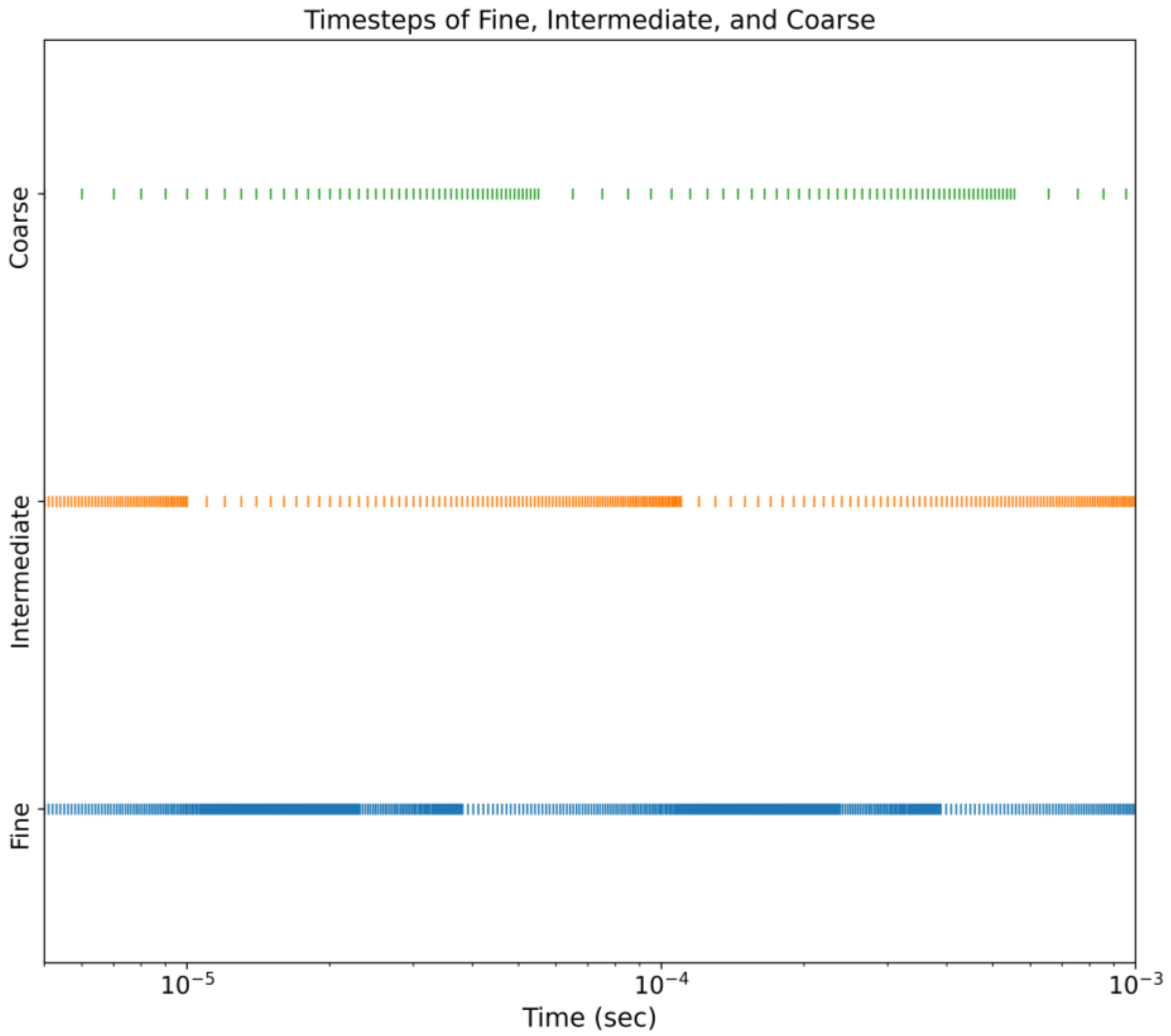
For the temporal discretization, it is a good practice to start with short time steps at the early times when the electromagnetic fields change rapidly [65]. At later stages, the time steps can be increased as the variations in the EM fields are more gradual and the signal-to-noise ratio (S/N) decreases. Shorter time steps increase the accuracy of the forward model but also the calculation time. Hence, it is important to find an adequate trade-off between accuracy and computational cost. In this paper, we tested three sets of temporal discretization with increased minimum and average size for the time steps (Table 1 and Figure 2).

Table 1.
Description of the different temporal discretization. F (fine), I (intermediate) and C (coarse) are the corresponding acronyms.
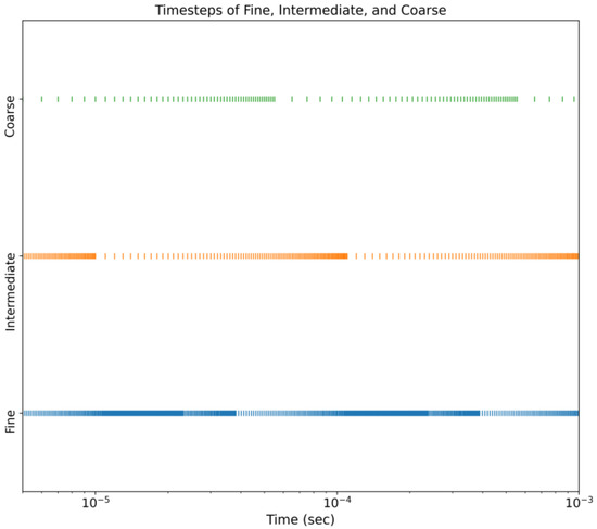
Figure 2.
Visual representation of the time discretization. The Y-axis shows the time discretization and the X-axis shows the logarithmic scale of the time-step size.
2.2.2. Spatial Discretization
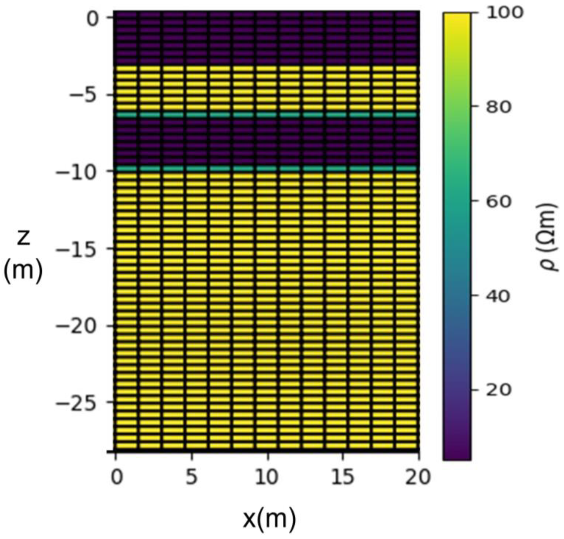
Spatial discretization also has a direct impact on the accuracy of the forward solver [65]. When creating the mesh, as shown in Figure 3, the discretization in the vertical direction is controlled by the cell size in the z-direction, whereas the horizontal discretization is controlled by the cell size in the x-direction. A finer discretization results in a more accurate solution but is also more computationally demanding. Note that a coarse discretization might also prevent an accurate representation of the layer boundaries as defined in the prior. If the layer boundary does not correspond to the edge of the mesh, a linear interpolation is used. In this paper, we selected five values for the vertical discretization to test the impact of the spatial discretization on the estimated posterior (Table 2).

Figure 3.
Example of the cylindrical mesh used for the forward model with a vertical discretization of 0.5 m and a horizontal discretization of 1.5 m. The cells with positive z represent the air, and are modelled with a very high resistivity and logarithmically increasing cell size.
Table 2.
Cell size in z-direction for the different spatial discretization. The letters in brackets, VF (very fine), F (fine), M (medium), C (coarse) and VC (very coarse) are used as acronyms in the remainder of this paper.
2.3. Synthetic Benchmark
We analysed the impact of both temporal and spatial discretization on the accuracy of the posterior distribution for all fifteen combinations of the temporal and spatial discretization (see Table 1 and Table 2), using synthetic data. A single combination is referred to by its acronyms, starting with the time discretization. The combination F-C, for example, corresponds to the fine time discretization combined with the coarse spatial discretization.
The synthetic data set is created with the finest discretization using the benchmark model parameters in brackets (see Table 3) defined by a five-layer model, with the last layer having an infinite thickness. The posterior distribution obtained with that same discretization and BEL1D-IPR is used as a reference. The prior is also the same for all tests and consists of uniform distributions for the nine model parameters (Table 3). The acquisition settings mimic the field set-up; see the following subsection.
Table 3.
Prior range of values for all parameters of the model. Benchmark model parameters for the synthetic model are shown in brackets.
3. Field Site
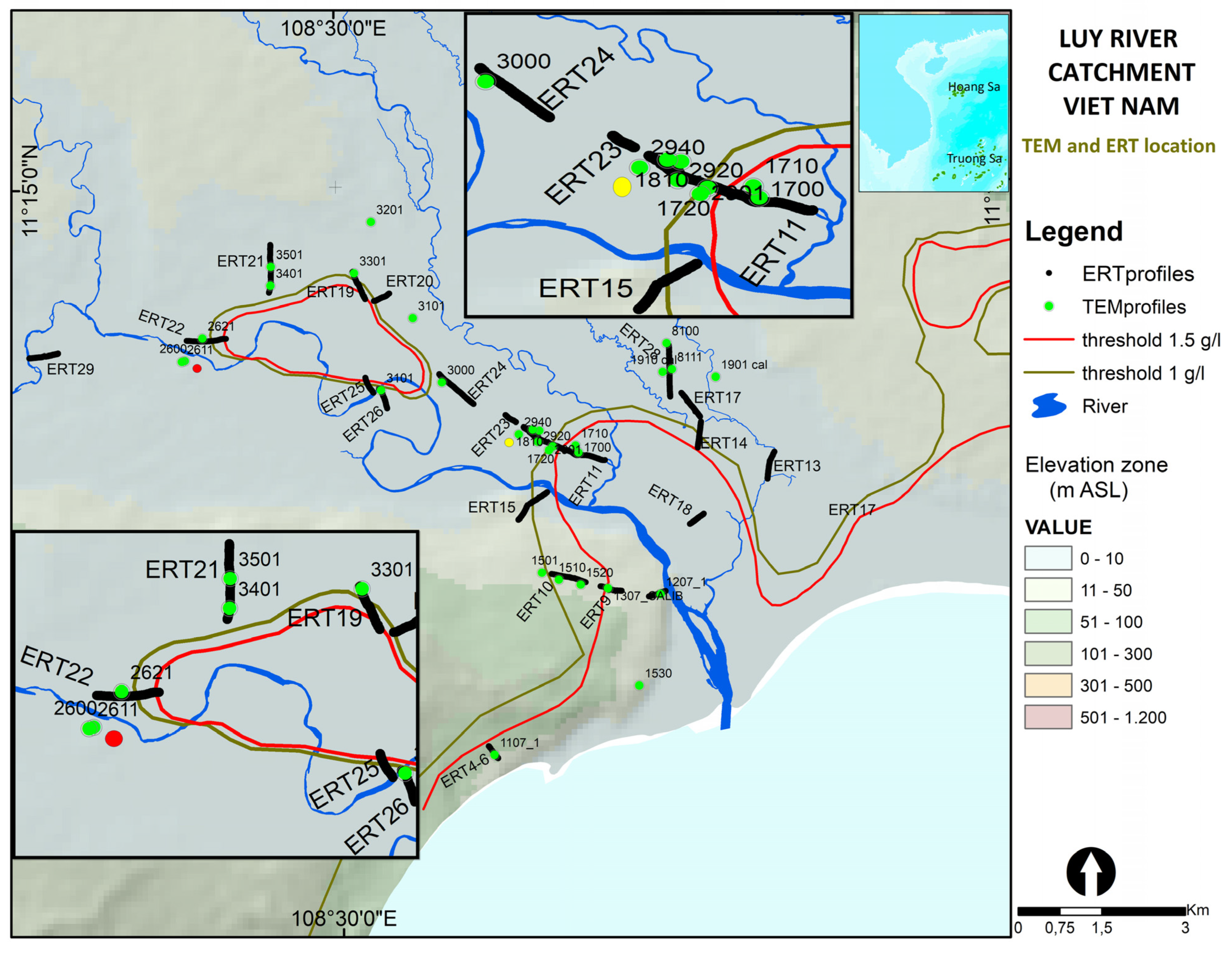
Understanding the interactions between salt and freshwater dynamics is crucial for managing coastal aquifers, yet it is difficult due to the required subsurface information, with high spatial and temporal resolution not always accessible from borehole data. The study area for the field tests is located in the Luy River catchment in the Binh Thuan province (Vietnam, Figure 4), which has been facing saltwater intrusions problems for many years [68,69,70].
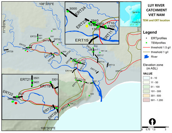
Figure 4.
The Luy River catchment in Vietnam with location of TDEM soundings (green points) and ERT profile (black line). The red and yellow dots represent the location of the soundings (2611 and 1307) used in this paper [68,69].
The data were collected using the TEM-FAST 48 equipment (Applied Electromagnetic Research, Utrecht, The Netherlands), with a 25 m square loop with a single turn acting as both transmitter and receiver. The injected current was set to 3.3 A with a dead-time of 5 µs. The data were collected using 42 semi-logarithmic time windows ranging from 4 µs to 4 ms. The signal was stacked allowing for noise estimation. A 50 Hz filter was applied to remove noise from the electricity network. For the inversion, the early time and late time were manually removed (see Section 4.3 and Section 4.4). The recorded signals at an early time steps, i.e., below 10−5 µs, were impacted by the current switch-off phenomena, while above 1 ms the signal-to-noise ratio was too low. We therefore filtered the TDEM data to a time range from 8 µs to 500 µs. In the forward model, we implemented the current shut-off ramp from the TEM-FAST48 system following the approach proposed by [71].
4. Results
We subdivide the results into four subsections. In the first subsection, we analyse the impact of the accuracy of the forward solver on the accuracy of the posterior in BEL1D-IPR. In the second section, we test the impact of a threshold on the rRMSE applied after the first BEL1D iteration (BEL1D-T). The third subsection is dedicated to the selection of the prior. Finally, the last section corresponds to the application of BEL1D-T to the field data.
4.1. Impact of Discretization
In this section, we tested in total 15 combinations of temporal and spatial discretization to study their behaviour on both the computation time and the accuracy of the posterior distribution computed with BEL1D-IPR (four iterations). The reference used the finest time and spatial discretization (F-VF). Since the computational costs of BEL1D are directly related to the number of prior samples and the computational cost of running one forward model [19], computing the solution for the F-VF combination is more than 150 times more expensive that running it with the C-VC combination (Table 4). An initial set of 1000 models is used in the prior. All calculations and simulation were carried out on a desktop computer with the following specifications: Processor intel ® CORE TM i7-9700 CPU @ 3.00 GHz, RAM 16.0 GB.
Table 4.
Time (in seconds) to compute one forward model in SimPEG for the 15 combinations of time and space discretization. The red colour corresponds to posterior distributions whose mean is biased, whereas the blue colour represents an under- or overestimation of the uncertainty for the two shallowest layers.
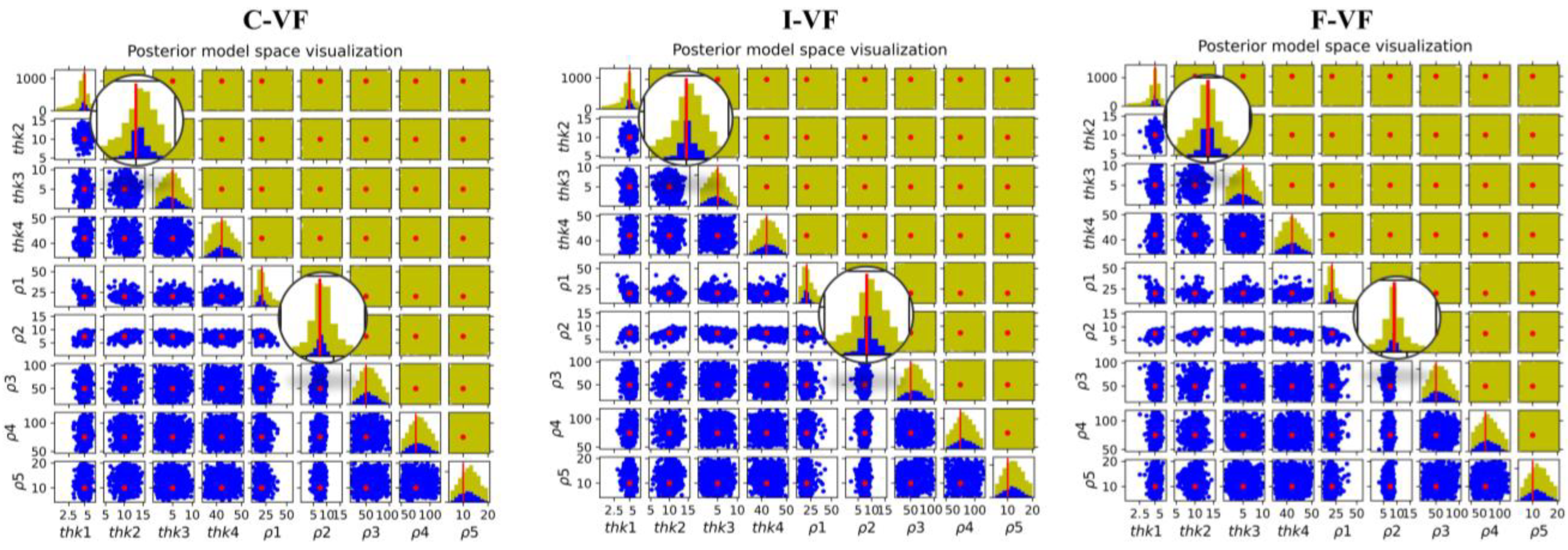
We first analyse the impact of the forward solver in BEL1D-IPR. A very similar behaviour is noted for all combinations using the VF spatial discretization, in combination with the three temporal discretization for all parameters (Figure 5). The parameters (thickness and resistivity) of the two first layers are recovered with relatively low uncertainty, while the uncertainty remains quite large for deeper layers, showing the intrinsic uncertainty of the methods related to the non-unicity of the solution. The results look globally similar, but a detailed analysis of the posterior distribution focusing on the resolved parameters (two first layers, see Figure 6) shows a slight bias of the mean value in C-VF and I-VF for the thickness of the second layer. This bias is small (less than 0.5 m) and could be the result of the sampling. A slightly larger uncertainty range can also be observed for the I and C time discretization.
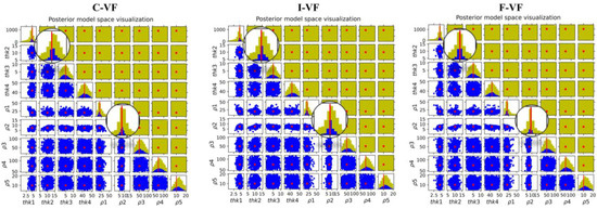
Figure 5.
Posterior model space visualization of fine-, intermediate-, and coarse-time discretization with very fine spatial discretization symbolized as C-VF, I-VF and F-VF. Thickness in meters and resistivity in ohm.m. Yellow dots correspond to prior models, blue dots to posterior models.
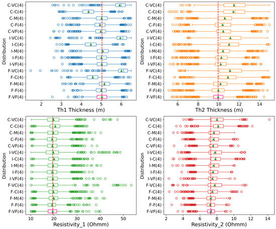
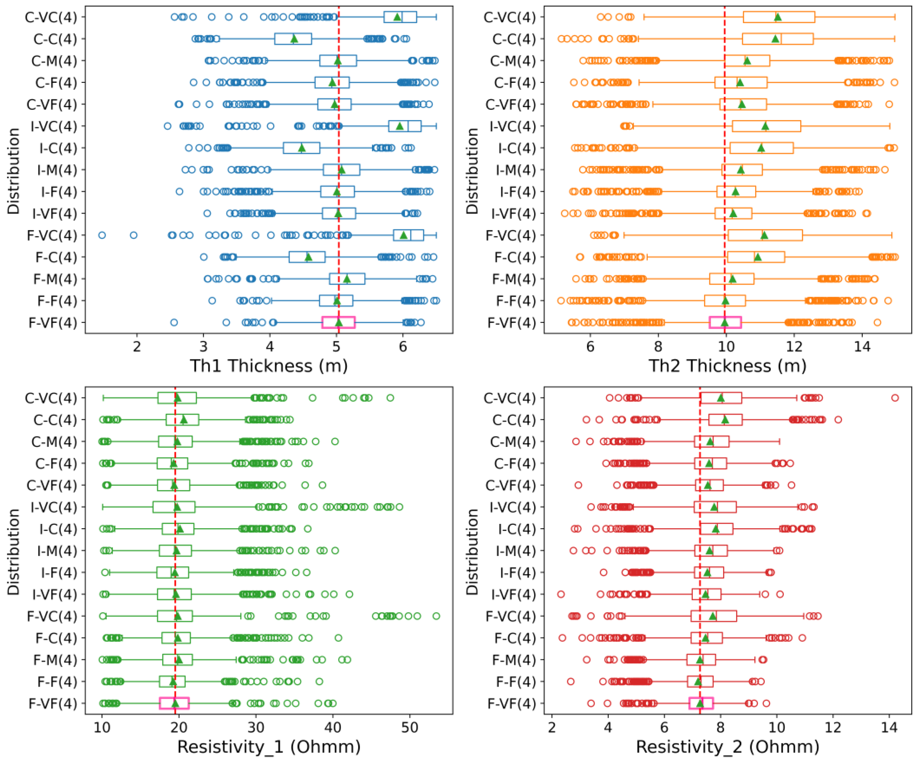
Figure 6.
Box plot of thickness and resistivity for the two first layers for BEL-IPR (four iterations). The red line shows the benchmark value and the F-VF(4) is the reference solution.
Globally, a systematic bias is observed for the largest spatial discretization (VC and C) for the thickness of layers 1 and 2 (Figure 6), which can likely be attributed to the difficulty in properly representing thin layers with a coarse discretization. A bias in the thickness of layer 2 is also noted for all coarse-time discretization, and to a lesser extent for the intermediate-time discretization, although this is limited when combined with F and VF spatial discretization. There is no significant bias visible in the estimation of the resistivity of layer 1, while most combinations have a small but not significant bias for layer 2, and the uncertainty range tends to be overestimated or underestimated for most combinations with large spatial discretization. Eventually, combinations with a VF or F spatial discretization combined with all time discretization, as well as the F-M combination, provide relatively similar results to the reference F-VF.
The time and spatial discretization for simulating the forward response of TDEM have therefore a strong impact, not only on the accuracy of the model response, but also on the estimation of the parameters of the shallow layers after inversion. In particular, the coarser spatial discretization biases the estimation of the thicknesses of the shallow layer. The same is also observed for the combination of a coarse- or intermediate-time discretization with a medium spatial discretization. As shallow layers correspond to the early times, this bias is likely related to an inaccurate simulation of the early TDEM response by the forward solver due to the chosen discretization. Although it comes with a high computation cost, we recommend keeping a relatively fine time and space discretization to guarantee the accuracy of the inversion. The cheapest option in terms of computational time with a minimum impact on the posterior distribution corresponds in this case to the C-F combination.
4.2. Impact of the Threshold
Because of the additional costs associated with the iterations, we compare the posterior distributions obtained with BEL1D-IPR to our new BEL1D-T approach, applying a threshold after the first iteration. The selected threshold based on the rRMSE calculated on the logarithm of the data are 0.18, 0.135, 0.05, corresponding, respectively, to a systematic error on the data of 20%, 15% and 5%. Various values of the threshold are tested for the reference solution (F-VF discretization) (Figure 7) and the analysis of the discretization is repeated (Figure 8). The threshold is applied after the first iteration to avoid additional computational time. The corresponding posterior distribution retains only the models that fit the data to an acceptable level. Note that the corresponding posterior distribution has a lower number of models than the IPR on BEL1D, as the latter enriches the posterior with iterations.
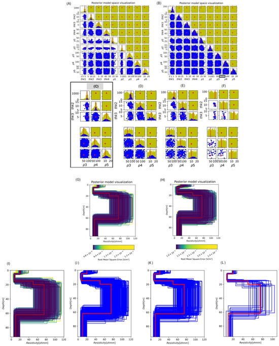
Figure 7.
Posterior-model space visualization: yellow dots represent the prior distribution, blue dots show the posterior distribution, and the red line corresponds to the benchmark model. The panels represent the following: (A) the posterior-model space distribution after four iterations without a threshold (BEL1D-IPR); (B) the posterior-model space distribution after one iteration without threshold. Comparison between BEL1D-IPR (C) and three threshold values for BEL1D-T (0.18, 0.135 and 0.05 (D–F)). The x and y axes are equivalent to resistivity (ohm.m) and depth (m). Posterior-model distribution for BEL1D-IPR (G,I) and after one iteration without a threshold (H) (the color scale is based on the value of the RMSE) and BEL1D-T with threshold values (0.18, 0.135 and 0.05, J–L).
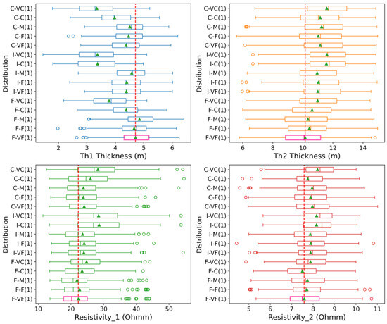
Figure 8.
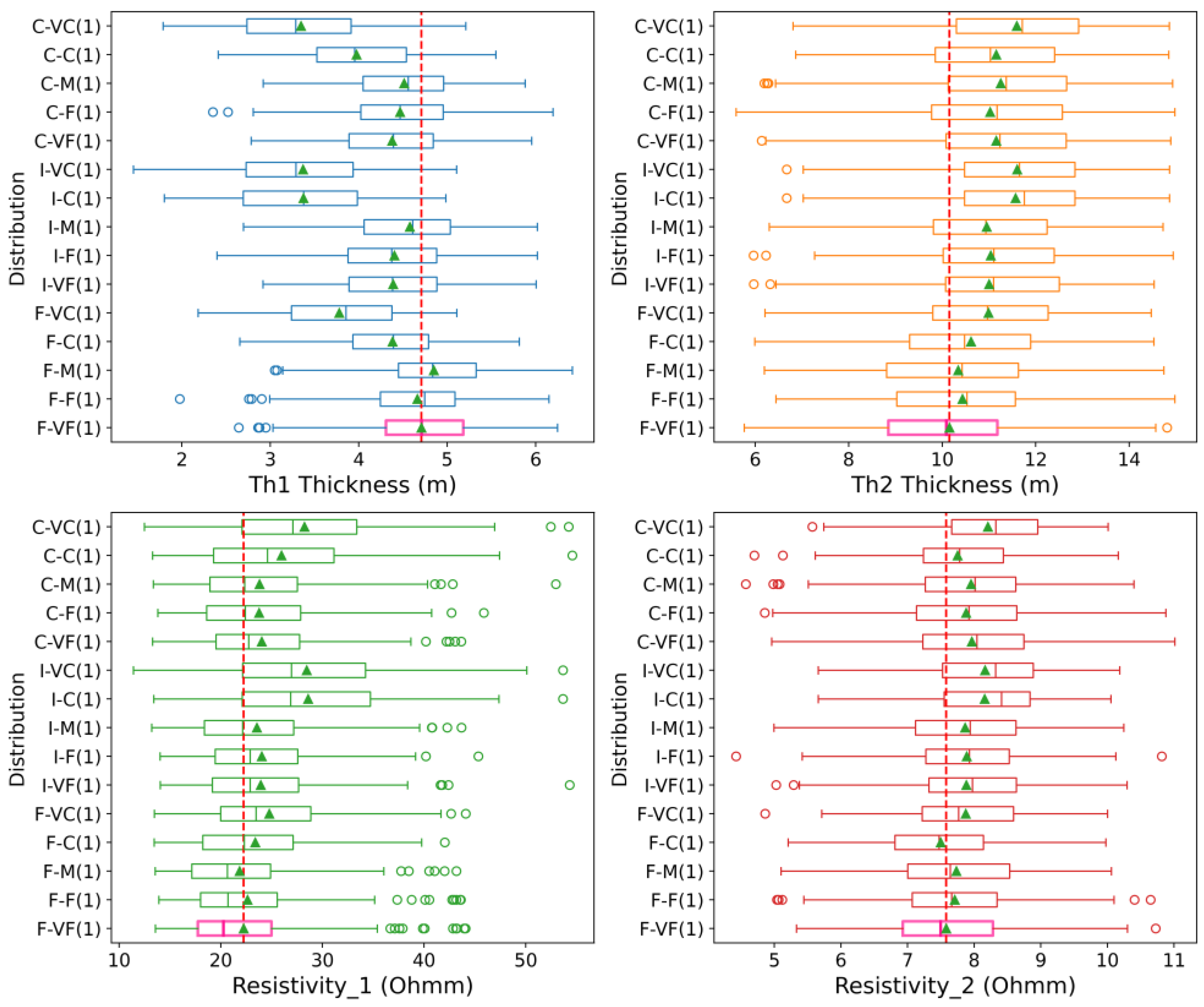
Box plot of thickness and resistivity for the two first layers after one iteration. Red line shows the benchmark F-VF (1). (1) represents the first iteration.
For solutions without a threshold, the colour scale is based on the quantiles of the RMSE in the posterior distribution. The threshold thus removes the models with the largest RMSE (yellow-green). Without the threshold (Figure 7A,B,G), some models not fitting the data are present in the posterior. The threshold approach after one iteration succeeds in obtaining a posterior closer to the reference solution (Figure 7D–F,J–L). The benchmark model, which is the true model, lies in the middle of the posterior.
The impact of the selected threshold value on the posterior distribution is illustrated in Figure 7D–F,J–L. Since the threshold is based on the rRMSE, decreasing its value is equivalent to rejecting the models with the largest data misfit from the posterior, while only models fitting the data with minimal variations are kept in the posterior. This rejection efficiently removes poor models from the posterior. If a low value is selected, only the very few best-fitting models are kept, and these are very similar to the reference model, hence reducing the posterior uncertainty range in the selected models (overfitting), while a high value of the threshold might retain models that do not fit the data within the noise level. The choice of the threshold should therefore be carefully made based on the noise level, and its sensitivity should be assessed.
Since the choice of the threshold impacts the rejection rate, the number of samples to generate cannot be estimated a priori. An initial estimate can, however be derived from a limited set of posterior samples. For the selected threshold value of 0.135, only 166 models are retained after filtering, corresponding to a rejection rate of 83.4%. If more models are required in the posterior, it is necessary to generate new models, which is not computationally expensive in BEL1D. The only additional effort is to compute the resulting rRMSE. The total computational effort is therefore proportional to the efficiency of the forward solver (Table 4). For instance, generating 500 models in the posterior would require generating 3000 samples based on the same rejection rate, and therefore would take three- times longer. BEL1D-T is therefore equivalent to a smart sampler that quickly generates models only in the vicinity of the posterior distribution and can contribute to a first fast assessment of the posterior. If the generation of many models is required, we rather recommend using BEL1D-IPR.
In this case, the threshold value of 0.135 seems acceptable and close to the BEL1D-IPR posterior distribution after four iterations. A higher threshold seems to retain too many samples, resulting in an overestimation of the posterior. The threshold value of 0.05 corresponds to a very large rejection rate and would require generating more models to assess the posterior properly. In the remaining part of the paper, the threshold 0.135 is used. The visualization of model space encompassing all combinations of temporal and spatial discretization for the first two layers’ thicknesses is illustrated in Figure S1 of the Supplementary Materials. Correspondingly, the depth-resistivity models are depicted in Figure S2 for the combinations of F-F, C-F, F-M, C-M, F-VC, and C-VC.
Figure 8 shows the boxplot results for BEL1D-T with the threshold 0.135 for various combinations of the discretization, and can be compared to the corresponding solution with BEL1D-IPR (Figure 6). Differences are less pronounced than with BEL1D-IPR. The F-VF and F-F and F-M discretization have similar posterior distributions as the reference for the thickness of the first two layers, while the uncertainty range for the resistivity is slightly underestimated. Figure 6 shows that the F-VF and F-F and F-M discretizations lead to results without bias for any parameters.
As with BEL1D-IPR, the very-coarse and coarse discretization are systematically biased. Most other combinations show a slight bias for the thickness of layer two, and—to a certain extent—also for layer one. Nonetheless, the difference with the reference for many combinations is less pronounced than for BEL1D-IPR. For example, the I-M and C-M combinations give relatively good approximations of the posterior. As in BEL1D-IPR the prior distribution is complemented with models sampled at the first iteration, without relying on their RMSE, an initial bias resulting from an error in the forward solver might be amplified in later iterations, leading to larger discrepancy between the response of the final model and the data. With BEL1D-T, the application of the threshold after iteration one prevents the solution deviating too much from the truth.
4.3. Impact of the Prior
In this section, we present some results obtained from the application of BEL1D to the TEM-fast dataset collected at sounding 2611, near project 22 (Figure 4). The measured signal can be seen in Figure 9, together with the standard deviation of the stacking error. A deterministic inversion of the data was carried out with SimPEG to have a first estimate of the electrical resistivity distribution (Figure 9). It shows a conductive zone at a shallow depth, likely corresponding to the saline part of the unconsolidated aquifer, while more resistive ground is found below 15 m, likely corresponding to the transition to the resistive bedrock. Below, a gradual decrease in resistivity can be observed.
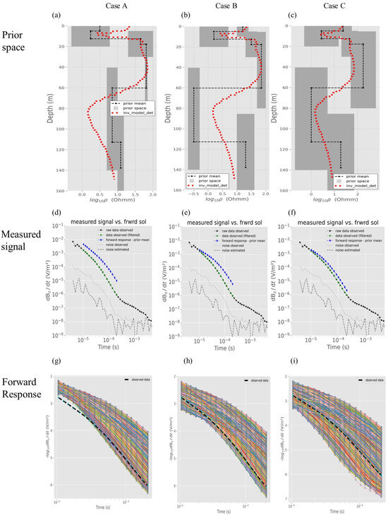
Figure 9.
Prior distributions for the three cases of sounding 2611. Case A: obvious inconsistent prior range; case B: slightly inconsistent prior range; case C: acceptable prior range. (a–c) Prior range with deterministic inversion (red); (d–f) measured signal, noise and forward solution for the prior mean; (g–i) forward response of each prior model.
In field cases, defining the prior distribution can be complicated, as the resistivity is not known in advance. We compare three possible prior combinations (obviously inconsistent prior range—case A, slightly inconsistent prior range—case B, acceptable prior range—case C) to better understand the impact of the choice of the prior. We apply BEL1D-T to bypass the additional computational time required in BEL1D-IPR, and use the F-F discretization.
The prior model consists of layers: the first five layers are characterized by their thickness and electrical resistivity, while the last layer has an infinite thickness. The prior distributions are shown in Figure 9 and Table 5. In case A, the prior is narrow, and was chosen to represent the main trend observed in the deterministic inversion. However, the first layers (upper 10 m) have a small resistivity range not in accordance with the deterministic inversion (red line in Figure 9). Similarly, the fourth layer underestimates the range of resistivity values expected from the deterministic inversion (60–70 Ohm.m). The prior for case B displays larger uncertainty: the first layer is forced to have larger resistivity values, and a strong transition is forced for the half-space. Finally, the last prior case C is very wide and allows a large overlap between successive layers, as well as a very large range of resistivity values.
Table 5.
Prior distributions for the different cases: (a) obviously inconsistent prior range, (b) slightly inconsistent prior range and (c) acceptable prior range.
The forward responses of the mean prior model of each three cases are displayed in Figure 9d–f. We can see that the response of the prior is the following: (1) it largely deviates from the measured signal for case A, (2) it deviates at later times for case B, and (3) it has the lowest deviation in case C. We also display the range of the forward response for 4000 prior models (Figure 9g–i). Due to the poor selection of the prior, a large difference between the measured data and the prior data space can be seen for case A (Figure 9g). The prior is clearly not consistent with the data, as the latter lies outside of the prior range in the data space in the early time steps. On the other hand, for case B (Figure 9h), the prior data range now encompasses the observed data, although it is rather at the edge of the prior distribution. For case C (Figure 9i), the prior range in the data space encompasses the measured data which lie close to the response of the prior mean model (Figure 9).
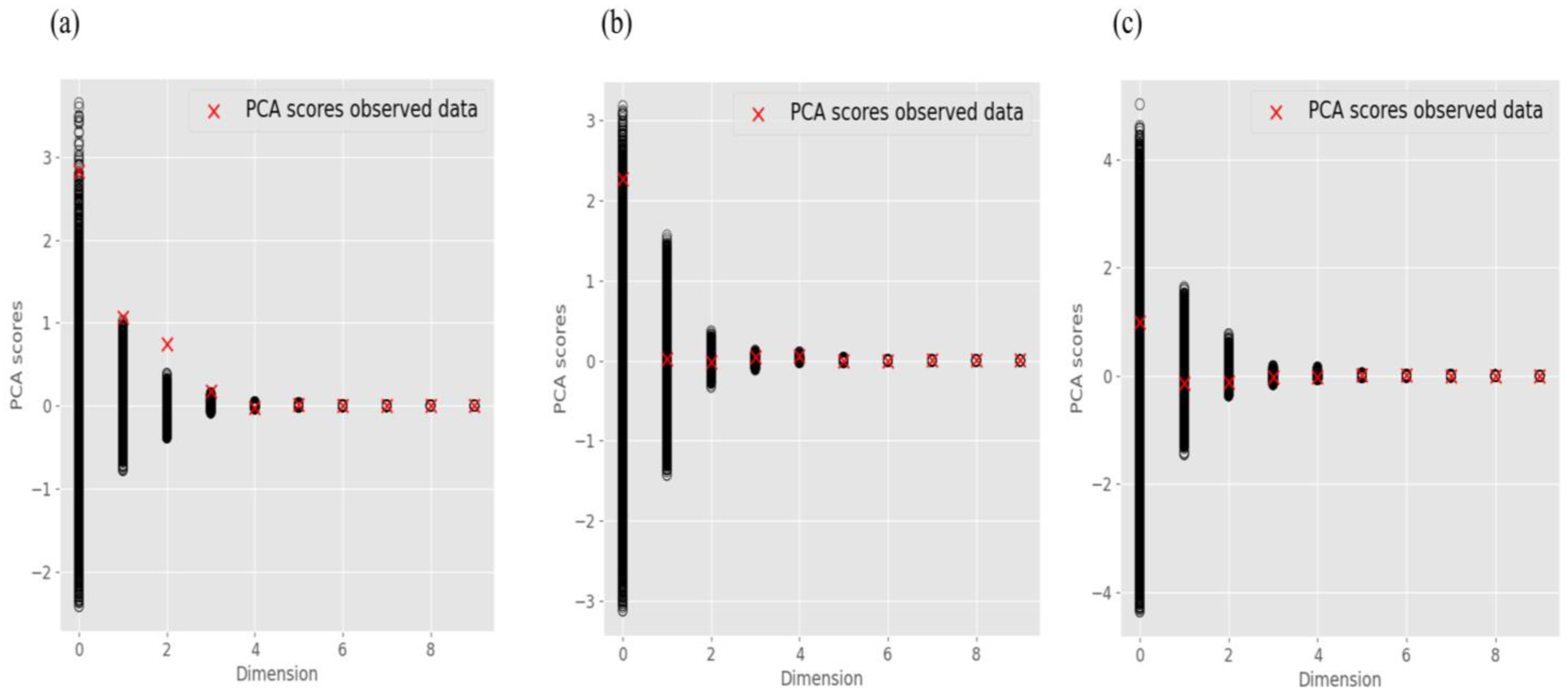
However, visual inspection is not sufficient to verify the consistency of the prior. Indeed, it is necessary to ensure that specific behaviours of the measured data can be reproduced by the prior model. This can be carried out more efficiently in the reduced PCA and CCA space [72]. Indeed, as BEL1D relies on learning, it cannot be used for extrapolation, and should not be used if the data fall outside the range of the prior. To further support the argument, the PCA and (part of) the CCA spaces are shown in Figure 10 and Figure 1, respectively. In Figure 10, the red crosses show the projection of the field data on every individual PCA dimension. It confirms that the prior for case A is inconsistent, with dimensions 2 and 3 lying outside, whereas the first PCA score lies at the edge of the prior distribution. For higher dimensions, the observed data lie within the range of the prior data space, but those dimensions represent only a limited part of the total variance. This is an indication that the prior is not able to reproduce the data and is therefore inconsistent. For cases B and C, no inconsistency is detected in the PCA space.
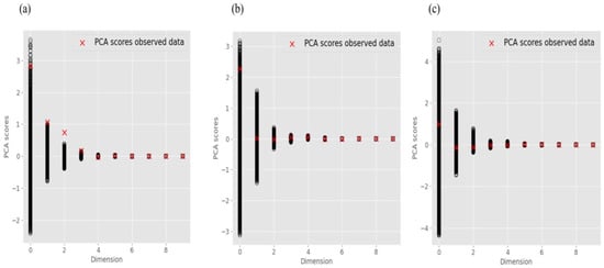
Figure 10.
PCA space, (a) obvious inconsistent prior, (b) slightly inconsistent prior and (c) acceptable prior. The black dot represents the prior models and the red cross represents the observed data.
A similar exercise is then performed in the CCA space where the projection of the field data is marked by a red line. In Figure 11a the observed data (red line) are lying outside the zone covered by the sampled prior models for most dimensions (grey zone). In such a case, BEL1D returns an error message and does not provide any estimation of the posterior. For the sake of illustration, we deactivated this preventive action and, nevertheless, performed the inversion. The posterior models in Figure 12 (case A) show low uncertainty for layers 1, 2, 4, 5, and 6, because of the limited range provided in the prior. The posterior data space shows that the posterior models do not fit the data, as a result of the inability of BEL to extrapolate in this case. Note that the threshold was not applied in this case, as it would have left no sample in the posterior, since none of them fit the observed data.
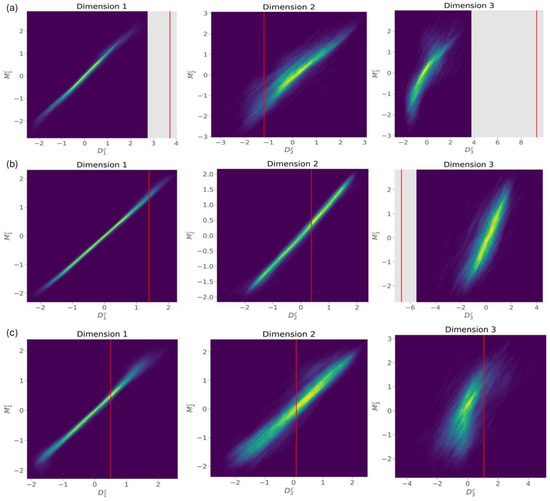
Figure 11.
CCA space for the three first dimensions, (a) obviously inconsistent prior, (b) slightly inconsistent prior and (c) acceptable prior. The red line represents the observed data. The y-axis corresponds to the reduced models and the x-axis corresponds to the reduced data.
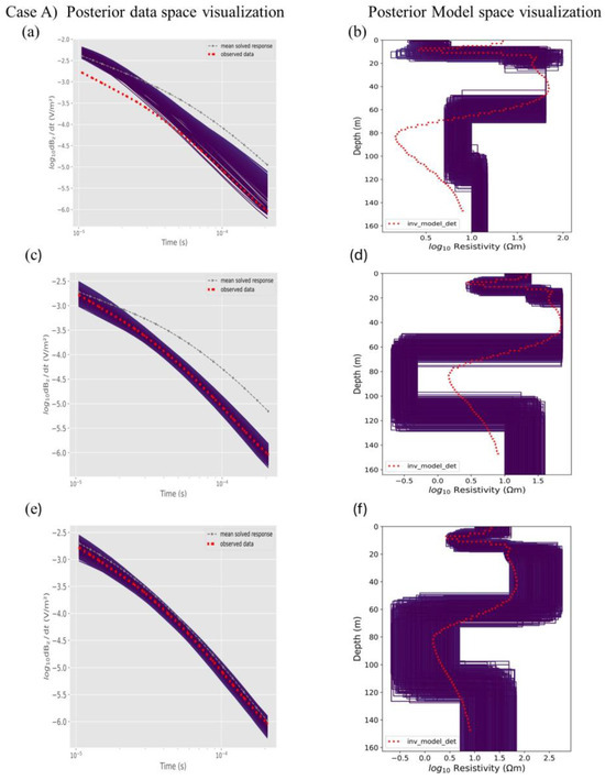
Figure 12.
Response of both posterior data and model space for the three prior selections: (a,b) obviously inconsistent prior range (without application of the threshold, (c,d) slightly inconsistent prior range, (e,f) acceptable prior range.
For case B, although it is apparently consistent in the PCA space, a similar occurrence of inconsistency appears in the CCA space (Figure 11b) for dimension three and some higher dimensions. Although apparently consistent with each individual dimension, the observed data do not correspond to combinations of dimensions contained in the prior, in which case they constitute an outlier for the proposed prior identified in the CCA space. However, in this case, the posterior models that are generated fit the data and have a relatively low RMSE (Figure 12c,d). The posterior-model visualization shows a limited uncertainty reduction for layers one to three and almost no uncertainty reduction for layers four, five and six (Figure 12c,d), likely pointing to a lack of sensitivity of the survey to these deeper layers. This indicates that BEL1D-T can overcome some inconsistency between the prior definition and the observed data, likely because the affected dimensions are only responsible for a small part of the total variance, to a level relatively similar to the noise level.
In case C, no inconsistency is detected in the prior data space, the PCA and CCA space (Figure 10c and Figure 11c). The posterior models do fit the data within the expected noise level and the deterministic inversion lies within the posterior (Figure 12e,f). The posterior uncertainty is large, especially for deeper layers (four, five and six). Therefore, in this case, BEL1D-T seems to correctly identify the posterior distribution of the model parameters. As the late times were filtered out, the data set is more sensitive to the shallow layers, and insensitive to the deeper layers. Increasing the prior range for those layers would also induce an increase in uncertainty in the posterior model.
4.4. Field Soundings
We selected two TDEM soundings, which are co-located with ERT profiles (red and yellow dots on Figure 4). The comparison with independent data can be used to evaluate the posterior solution from BEL1D-T. For the TDEM soundings (see Figure 13c,d), we compare the deterministic inversion, the BEL1D-T posterior distribution and a conductivity profile extracted from the ERT profile at the location of the sounding.

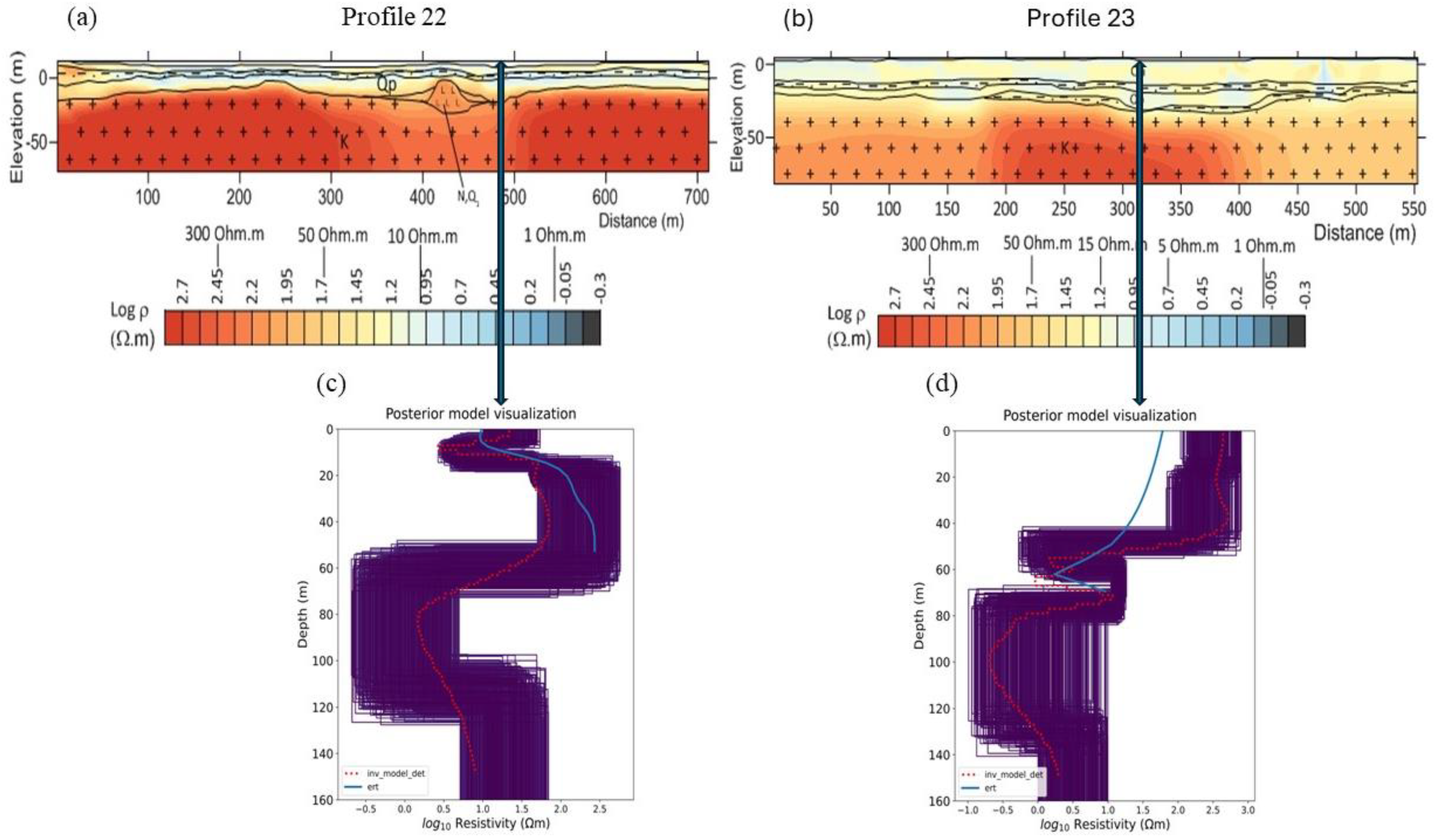
Figure 13.
(a) ERT profile 22 near to the Luy River; (b) ERT profile 23 near the dunes. Posterior model visualization for TDEM soundings on profile 22 (c) and 23 (d). ERT inversion in blue and deterministic inversion of TDEM data in red.
The resistivity image and TDEM results of profile 22 show the same trend (Figure 13a,c). At a shallow depth between 5 and 15 m, less-resistive layers are observed, which indicates the presence of saltwater in the unconsolidated sediment (20 to 25 m thickness). At a greater depth, we have an increase in resistivity corresponding to the transition to the bedrock. The deterministic solution tends to show a decrease in resistivity at greater depths, which may be an artifact due to the loss of resolution. BEL1D-T is successful in providing a realistic uncertainty quantification, not resolved with the deterministic inversion. It can be observed that, except for the shallow layer, the reduction in uncertainty compared to the prior is relatively limited and concerns mostly the thickness and not the resistivity, illustrating the insensitivity of the survey set-up for depths below 60 m, where the solution is mostly driven by the definition of the prior distribution. The selection of an rRMSE threshold, however, ensures that all those models are consistent with the recorded data.
The results for profile 23 are different (Figure 13b,d). This site is at the foot of sand dunes, close to the sea, with an elevation level between 11 and 50 m. The shallow layer is relatively resistive, but the two methods do not agree on the value of the resistivity, with the TDEM resulting in higher values. BEL1D-T tends to predict a larger uncertainty towards low values of the resistivity for the shallow layers compared to the deterministic inversion. Below 50 m, the resistivity drops to 1–10 Ohm.m for both methods, which seems to show the presence of saltwater in the bedrock. The uncertainty range estimated by BEL1D-T seems to invalidate the presence of rapidly varying resistivity between 50 and 75 m, predicted by the deterministic TDEM inversion, which is quite coherent with the lack of sensitivity at this depth.
4.5. Summary and Discussion
Deterministic inversions are affected by the non-uniqueness of the solution preventing the quantification of uncertainty. Our approach using BEL1D-T allows us to retrieve not only the changes in resistivity with depth, but also to quantify the reliability of the model. We summarize the main outcomes of the sections above as the following:
- (1)
- When using a numerical forward model, the temporal and spatial discretization have a significant effect on the retrieved posterior distribution. A semi-analytical approach is recommended when possible. Otherwise, a sufficiently fine temporal and spatial discretization must be retained and BEL1D-T constitutes an efficient and fast alternative for computing the posterior distribution.
- (2)
- BEL1D-T is an efficient and accurate approach for predicting uncertainty with limited computational effort. It was shown to be equivalent to BEL1D-IPR but requires fewer forward models to be computed.
- (3)
- As with any Bayesian approach, BEL1D-related methods are sensitive to the choice of the prior model. The consistency between the prior and the observed data is integrated, and the threshold approach allows for quickly identifying the inconsistent posterior model. We recommend running a deterministic inversion to define the prior model while keeping a wide range for each parameter, allowing for sufficient variability. Our findings illuminate the substantial uncertainty enveloping the deterministic inversion, highlighting the risk of disregarding such uncertainty, particularly in zones of low sensitivity at greater depths. We implement a threshold criterion to ensure all the models within the posterior distribution fit the observed data within a realistic error. Nonetheless, there exists a risk of underestimating uncertainty when the prior distribution is overly restrictive, as detailed in our prior analysis. Relying too much on the deterministic inversion is therefore dangerous, as it might not recover some variations occurring in the field because of the chosen inversion approach. To accommodate a broader prior, it may be imperative to resort to BEL1D-IPR or to increase the sample size significantly, ensuring a comprehensive exploration of the model space and a more accurate reflection of the inherent uncertainties.
- (4)
- For the field case, the results are consistent with ERT and deterministic inversion. Our analysis reveals that the uncertainty reduction at depths greater than 60 m is almost non-existent. It is recommended to avoid interpreting the model parameters at that depth, as the solution is likely highly dependent on the prior.
5. Conclusions
In this paper, we introduce a new approach combining BEL1D with a threshold after the first iteration (BEL1D-T) as a fast and efficient stochastic inversion method for TDEM data. Although BEL1D-T only requires a limited number of forward runs, the computational time remains relatively important as we used the numerical solver of SimPEG to calculate the forward response. The proper selection of time-steps and space discretization is essential to limit the computation cost while keeping an accurate posterior distribution. Our numerical studies reveal that there is a compromise between the spatial and temporal discretization in the forward solver that minimizes the ricks of numerical errors in the posteriors generated, yet also reducing the computational cost. A fine temporal discretization seems to be important, as described in Table 1, yet a very fine spatial discretization does not seem mandatory. As this analysis is likely specific to every acquisition set-up and prior distribution, we suggest carefully evaluating the modelling error introduced by the forward model before starting the BEL1D-T inversion. The use of faster semi-analytical forward models is recommended when available. However, 2D and 3D effects when the 1D forward solver are used are expected to have a similar impact on the forward-model error. as observed in our work.
The application of a threshold on the rRMSE after one iteration is an efficient approach to limiting the computational costs. We select the threshold based on the estimated relative error in the data set, translated into an absolute value of the rRMSE calculated on a log scale. Selecting a too-selective threshold can result in overfitting and thus an underestimation of the uncertainty. We showed that selecting a threshold based on the expected noise level leads to a solution similar to the one obtained with the reference BEL1D-IPR. The proposed approach allows for partly mitigating the adverse effects of an inaccurate forward model, and therefore can be used to obtain a first fast assessment of the posterior distribution.
Moreover, it should be noted that, as with any stochastic methods, BEL1D is sensitive to the definition of the prior. We have experienced some prior distributions that might appear visually consistent in the data space resulting in inconsistencies in the low-dimensional spaces. It is thus crucial to verify the consistency of the prior also in the lower dimensional space. This feature is included by default in the pyBEL1D code [58], but it might be interesting to deactivate this feature in order to investigate the reasons and their impacts on the posterior. Beside the definition of the prior itself, the inconsistency can be attributed to the noisy nature of the field data [19].
In the case of large uncertainty, an iterative prior resampling approach is advised, as proposed by [19], but it comes at a larger computational cost. Therefore, we propose reducing the prior uncertainty by using the deterministic inversion as a guide, and limiting ourselves to the first iteration, while filtering the models based on their RMSE. However, care should be taken to avoid restricting the prior too much, as this might yield an underestimation of the uncertainty. In such cases, BEL1D-T acts more as a stochastic optimization algorithm, providing only a fast approximation of the posterior distribution, but still allowing for the rough estimation of the uncertainty of the solution, without requiring heavy computational power such as HPC facilities.
We validated the approach using TDEM soundings acquired in a saltwater intrusion context in Vietnam. The posterior distribution was consistent with both the deterministic inversion and the ERT profiles. The range of uncertainty was larger where TDEM and ERT deterministic inversions do not agree, which illustrates the intrinsic uncertainty of these type of data and the need for uncertainty quantification.
Supplementary Materials
The following supporting information can be downloaded at: https://www.mdpi.com/article/10.3390/w16071056/s1, Figure S1. (a) Posterior-model space visualization with one iteration and threshold (0.135), (b) posterior-model space visualization with four iterations; the above row is with fine-time discretization, whereas the other rows are with intermediate- and coarse-time discretization. From left to right, with spatial discretization (VF, F, M, C, and VC). Figure S2. Posterior-model visualization with respect to depth (m) vs resistivity (ohm.m); colour bar represents the RMSE values (a) with four iterations without a threshold and (b) with one iteration and a 0.135 threshold value.
Author Contributions
The conceptualization of this project was led by T.H., with the contribution of A.A., D.D. and A.F.O. The methods were developed by H.M. (implementation of BEL1D and BEL1D-IPR), A.A. (BEL1D-T link SimPEG forward solver), L.A. and W.D. (linking the SimPEG forward solver with BEL1D-IPR). A.A. ran all simulations (discretization, threshold, prior selection, and field data). The initial draft was written by A.A. with significant input from T.H. All authors edited and reviewed the draft. T.H. and D.D. provided supervision for A.A. throughout the whole research project. Project administration: T.H., and funding acquisition: A.A. and T.H. All authors have read and agreed to the published version of the manuscript.
Funding
AA: was funded by the Higher Education Commission (HEC) of Pakistan, with the reference number 50028442/PM/UESTPs/HRD/HEC/2022/December 5, 2022, and from the Bijzonder Onderzoeksfonds (BOF) of Ghent University, with grant number BOF.CDV.2023.0058.01. WD was funded by the Fund for Scientific Research (FWO) in Flanders, with grants 1113020N and 1113022N and the KU Leuven Postdoctoral Mandate PDMt223065. HM was funded by the F.R.S,-FNRS, with grants 32905391 and 40000777.
Data Availability Statement
The field data can be made available upon request.
Acknowledgments
We thank Robin Thibaut for helping in the analysis and plotting of the PCA space. We thank Robin Thibaut, Linh Pham Dieu, Diep Cong-Thi and all the team from the VIGMR for field data collection.
Conflicts of Interest
The authors declare no conflicts of interest.
References
- Kemna, A.; Nguyen, F.; Gossen, S. On Linear Model Uncertainty Computation in Electrical Imaging. In Proceedings of the SIAM Conference on Mathematical and Computational Issues in the Geosciences, Santa Fe, NM, USA, 19–22 March 2007. [Google Scholar]
- Hermans, T.; Vandenbohede, A.; Lebbe, L.; Nguyen, F. A Shallow Geothermal Experiment in a Sandy Aquifer Monitored Using Electric Resistivity Tomography. Geophysics 2012, 77, B11–B21. [Google Scholar] [CrossRef]
- Parsekian, A.D.; Grombacher, D. Uncertainty Estimates for Surface Nuclear Magnetic Resonance Water Content and Relaxation Time Profiles from Bootstrap Statistics. J. Appl. Geophys. 2015, 119, 61–70. [Google Scholar] [CrossRef]
- Aster, R.; Borchers, B.; Thurber, C. Parameter Estimation and Inverse Problems; Academic Press: Cambridge, MA, USA, 2013. [Google Scholar]
- Sambridge, M. Monte Carlo Methods in Geophysical Inverse Problems. Rev. Geophys. 2002, 40, 3-1–3-29. [Google Scholar] [CrossRef]
- Yeh, W.W.-G. Review of Parameter Identification Procedures in Groundwater Hydrology: The Inverse Problem. Water Resour. Res. 1986, 22, 95–108. [Google Scholar] [CrossRef]
- McLaughlin, D.; Townley, L.R. A Reassessment of the Groundwater Inverse Problem. Water Resour. Res. 1996, 32, 1131–1161. [Google Scholar] [CrossRef]
- Hidalgo, J.; Slooten, L.J.; Carrera, J.; Alcolea, A.; Medina, A. Inverse Problem in Hydrogeology. Hydrogeol. J. 2005, 13, 206–222. [Google Scholar] [CrossRef]
- Zhou, H.; Gómez-Hernández, J.J.; Li, L. Inverse Methods in Hydrogeology: Evolution and Recent Trends. Adv. Water Resour. 2014, 63, 22–37. [Google Scholar] [CrossRef]
- Sen, M.K.; Stoffa, P.L. Bayesian Inference, Gibbs’ Sampler, and Uncertainty Estimation in Geophysical Inversion. Geophys. Prospect. 1996, 44, 313–350. [Google Scholar] [CrossRef]
- Tarantola, A. Inverse Problem Theory and Methods for Model Parameter Estimation; Society for Industrial and Applied Mathematics: Philadelphia, PA, USA, 2005. [Google Scholar]
- Irving, J.; Singha, K. Stochastic Inversion of Tracer Test and Electrical Geophysical Data to Estimate Hydraulic Conductivities. Water Resour. Res. 2010, 46, W11514. [Google Scholar] [CrossRef]
- Trainor-Guitton, W.; Hoversten, G.M. Stochastic Inversion for Electromagnetic Geophysics: Practical Challenges and Improving Convergence Efficiency. Geophysics 2011, 76, F373–F386. [Google Scholar] [CrossRef]
- De Pasquale, G.; Linde, N. On Structure-Based Priors in Bayesian Geophysical Inversion. Geophys. J. Int. 2017, 208, 1342–1358. [Google Scholar] [CrossRef]
- Ball, L.B.; Davis, T.A.; Minsley, B.J.; Gillespie, J.M.; Landon, M.K. Probabilistic Categorical Groundwater Salinity Mapping from Airborne Electromagnetic Data Adjacent to California’s Lost Hills and Belridge Oil Fields. Water Resour. Res. 2020, 56, e2019WR026273. [Google Scholar] [CrossRef]
- Bobe, C.; Van De Vijver, E.; Keller, J.; Hanssens, D.; Van Meirvenne, M.; De Smedt, P. Probabilistic 1-D Inversion of Frequency-Domain Electromagnetic Data Using a Kalman Ensemble Generator. IEEE Trans. Geosci. Remote Sens. 2020, 58, 3287–3297. [Google Scholar] [CrossRef]
- Tso, C.-H.M.; Iglesias, M.; Wilkinson, P.; Kuras, O.; Chambers, J.; Binley, A. Efficient Multiscale Imaging of Subsurface Resistivity with Uncertainty Quantification Using Ensemble Kalman Inversion. Geophys. J. Int. 2021, 225, 887–905. [Google Scholar] [CrossRef]
- Michel, H.; Hermans, T.; Kremer, T.; Elen, A.; Nguyen, F. 1D Geological Imaging of the Subsurface from Geophysical Data with Bayesian Evidential Learning. Part 2: Applications and Software. Comput. Geosci. 2020, 138, 104456. [Google Scholar] [CrossRef]
- Michel, H.; Hermans, T.; Nguyen, F. Iterative Prior Resampling and Rejection Sampling to Improve 1D Geophysical Imaging Based on Bayesian Evidential Learning (BEL1D). Geophys. J. Int. 2023, 232, 958–974. [Google Scholar] [CrossRef]
- Scheidt, C.; Renard, P.; Caers, J. Prediction-Focused Subsurface Modeling: Investigating the Need for Accuracy in Flow-Based Inverse Modeling. Math. Geosci. 2015, 47, 173–191. [Google Scholar] [CrossRef]
- Satija, A.; Scheidt, C.; Li, L.; Caers, J. Direct Forecasting of Reservoir Performance Using Production Data without History Matching. Comput. Geosci. 2017, 21, 315–333. [Google Scholar] [CrossRef]
- Hermans, T.; Nguyen, F.; Klepikova, M.; Dassargues, A.; Caers, J. Uncertainty Quantification of Medium-Term Heat Storage from Short-Term Geophysical Experiments Using Bayesian Evidential Learning. Water Resour. Res. 2018, 54, 2931–2948. [Google Scholar] [CrossRef]
- Athens, N.D.; Caers, J.K. A Monte Carlo-Based Framework for Assessing the Value of Information and Development Risk in Geothermal Exploration. Appl. Energy 2019, 256, 113932. [Google Scholar] [CrossRef]
- Thibaut, R.; Compaire, N.; Lesparre, N.; Ramgraber, M.; Laloy, E.; Hermans, T. Comparing Well and Geophysical Data for Temperature Monitoring within a Bayesian Experimental Design Framework. Water Resour. Res. 2022, 58, e2022WR033045. [Google Scholar] [CrossRef]
- Park, J.; Caers, J. Direct Forecasting of Global and Spatial Model Parameters from Dynamic Data. Comput. Geosci. 2020, 143, 104567. [Google Scholar] [CrossRef]
- Yin, Z.; Strebelle, S.; Caers, J. Automated Monte Carlo-Based Quantification and Updating of Geological Uncertainty with Borehole Data (AutoBEL v1.0). Geosci. Model Dev. 2020, 13, 651–672. [Google Scholar] [CrossRef]
- Tadjer, A.; Bratvold, R.B. Managing Uncertainty in Geological CO2 Storage Using Bayesian Evidential Learning. Energies 2021, 14, 1557. [Google Scholar] [CrossRef]
- Fang, J.; Gong, B.; Caers, J. Data-Driven Model Falsification and Uncertainty Quantification for Fractured Reservoirs. Engineering 2022, 18, 116–128. [Google Scholar] [CrossRef]
- Thibaut, R.; Laloy, E.; Hermans, T. A New Framework for Experimental Design Using Bayesian Evidential Learning: The Case of Wellhead Protection Area. J. Hydrol. 2021, 603, 126903. [Google Scholar] [CrossRef]
- Yang, H.-Q.; Chu, J.; Qi, X.; Wu, S.; Chiam, K. Bayesian Evidential Learning of Soil-Rock Interface Identification Using Boreholes. Comput. Geotech. 2023, 162, 105638. [Google Scholar] [CrossRef]
- Hermans, T.; Oware, E.; Caers, J. Direct Prediction of Spatially and Temporally Varying Physical Properties from Time-Lapse Electrical Resistance Data. Water Resour. Res. 2016, 52, 7262–7283. [Google Scholar] [CrossRef]
- Pradhan, A.; Mukerji, T. Seismic Bayesian Evidential Learning: Estimation and Uncertainty Quantification of Sub-Resolution Reservoir Properties. Comput. Geosci. 2020, 24, 1121–1140. [Google Scholar] [CrossRef]
- Heagy, L.J.; Cockett, R.; Kang, S.; Rosenkjaer, G.K.; Oldenburg, D.W. A Framework for Simulation and Inversion in Electromagnetics. Comput. Geosci. 2017, 82, WB9–WB19. [Google Scholar] [CrossRef]
- Cockett, R.; Kang, S.; Heagy, L.J.; Pidlisecky, A.; Oldenburg, D.W. SimPEG: An Open Source Framework for Simulation and Gradient Based Parameter Estimation in Geophysical Applications. Comput. Geosci. 2015, 85, 142–154. [Google Scholar] [CrossRef]
- Chongo, M.; Christiansen, A.V.; Tembo, A.; Banda, K.E.; Nyambe, I.A.; Larsen, F.; Bauer-Gottwein, P. Airborne and Ground-Based Transient Electromagnetic Mapping of Groundwater Salinity in the Machile–Zambezi Basin, Southwestern Zambia. Near Surf. Geophys. 2015, 13, 383–396. [Google Scholar] [CrossRef]
- Mohamaden, M.; Araffa, S.A.; Taha, A.; AbdelRahman, M.A.; El-Sayed, H.M.; Sharkawy, M.S. Geophysical Techniques and Geomatics-Based Mapping for Groundwater Exploration and Sustainable Development at Sidi Barrani Area, Egypt. Egypt. J. Aquat. Res. 2023, in press. [Google Scholar] [CrossRef]
- Rey, J.; Martínez, J.M.; Mendoza, R.; Sandoval, S.; Tarasov, V.; Kaminsky, A.; Morales, K. Geophysical Characterization of Aquifers in Southeast Spain Using ERT, TDEM, and Vertical Seismic Reflection. Appl. Sci. 2020, 10, 7365. [Google Scholar] [CrossRef]
- Siemon, B.; Christiansen, A.V.; Auken, E. A Review of Helicopter-Borne Electromagnetic Methods for Groundwater Exploration. Near Surf. Geophys. 2009, 7, 629–646. [Google Scholar] [CrossRef]
- Vilhelmsen, T.N.; Marker, P.A.; Foged, N.; Wernberg, T.; Auken, E.; Christiansen, A.V.; Bauer-Gottwein, P.; Christensen, S.; Høyer, A.-S. A Regional Scale Hydrostratigraphy Generated from Geophysical Data of Varying Age, Type, and Quality. Water Resour. Manag. 2018, 33, 539–553. [Google Scholar] [CrossRef]
- Goebel, M.; Knight, R.; Halkjær, M. Mapping Saltwater Intrusion with an Airborne Electromagnetic Method in the Offshore Coastal Environment, Monterey Bay, California. J. Hydrol. Reg. Stud. 2019, 23, 100602. [Google Scholar] [CrossRef]
- Auken, E.; Foged, N.; Larsen, J.J.; Lassen, K.V.T.; Maurya, P.K.; Dath, S.M.; Eiskjær, T.T. tTEM—A Towed Transient Electromagnetic System for Detailed 3D Imaging of the Top 70 m of the Subsurface. Geophysics 2019, 84, E13–E22. [Google Scholar] [CrossRef]
- Lane, J.W., Jr.; Briggs, M.A.; Maurya, P.K.; White, E.A.; Pedersen, J.B.; Auken, E.; Terry, N.; Minsley, B.K.; Kress, W.; LeBlanc, D.R.; et al. Characterizing the Diverse Hydrogeology Underlying Rivers and Estuaries Using New Floating Transient Electromagnetic Methodology. Sci. Total Environ. 2020, 740, 140074. [Google Scholar] [CrossRef] [PubMed]
- Aigner, L.; Högenauer, P.; Bücker, M.; Flores Orozco, A. A Flexible Single Loop Setup for Water-Borne Transient Electromagnetic Sounding Applications. Sensors 2021, 21, 6624. [Google Scholar] [CrossRef] [PubMed]
- Viezzoli, A.; Christiansen, A.V.; Auken, E.; Sørensen, K. Quasi-3D Modeling of Airborne TEM Data by Spatially Constrained Inversion. Geophysics 2008, 73, F105–F113. [Google Scholar] [CrossRef]
- Linde, N.; Ginsbourger, D.; Irving, J.; Nobile, F.; Doucet, A. On Uncertainty Quantification in Hydrogeology and Hydrogeophysics. Adv. Water Resour. 2017, 110, 166–181. [Google Scholar] [CrossRef]
- Josset, L.; Ginsbourger, D.; Lunati, I. Functional Error Modeling for Uncertainty Quantification in Hydrogeology. Water Resour. Res. 2015, 51, 1050–1068. [Google Scholar] [CrossRef]
- Scholer, M.; Irving, J.; Looms, M.C.; Nielsen, L.; Holliger, K. Bayesian Markov-Chain-Monte-Carlo Inversion of Time-Lapse Crosshole GPR Data to Characterize the Vadose Zone at the Arrenaes Site, Denmark. Vadose Zone J. 2012, 11, vzj2011.0153. [Google Scholar] [CrossRef]
- Calvetti, D.; Ernst, O.; Somersalo, E. Dynamic Updating of Numerical Model Discrepancy Using Sequential Sampling. Inverse Probl. 2014, 30, 114019. [Google Scholar] [CrossRef]
- Köpke, C.; Irving, J.; Elsheikh, A.H. Accounting for Model Error in Bayesian Solutions to Hydrogeophysical Inverse Problems Using a Local Basis Approach. Adv. Water Resour. 2018, 116, 195–207. [Google Scholar] [CrossRef]
- Deleersnyder, W.; Dudal, D.; Hermans, T. Multidimensional Surrogate Modelling for Airborne TDEM Data Accepted Pending Revision. Comput. Geosci. 2024. [Google Scholar] [CrossRef]
- Khu, S.-T.; Werner, M.G.F. Reduction of Monte-Carlo Simulation Runs for Uncertainty Estimation in Hydrological Modelling. Hydrol. Earth Syst. Sci. 2003, 7, 680–692. [Google Scholar] [CrossRef]
- Brynjarsdóttir, J.; O’Hagan, A. Learning About Physical Parameters: The Importance of Model Discrepancy. Inverse Probl. 2014, 30, 114007. [Google Scholar] [CrossRef]
- Hansen, T.M.; Cordua, K.S.; Jacobsen, B.H.; Mosegaard, K. Accounting for Imperfect Forward Modeling in Geophysical Inverse Problems—Exemplified for Crosshole Tomography. Geophysics 2014, 79, H1–H21. [Google Scholar] [CrossRef]
- Deleersnyder, W.; Maveau, B.; Hermans, T.; Dudal, D. Inversion of Electromagnetic Induction Data Using a Novel Wavelet-Based and Scale-Dependent Regularization Term. Geophys. J. Int. 2021, 226, 1715–1729. [Google Scholar] [CrossRef]
- Deleersnyder, W.; Dudal, D.; Hermans, T. Novel Airborne EM Image Appraisal Tool for Imperfect Forward Modelling. Remote Sens. 2022, 14, 5757. [Google Scholar] [CrossRef]
- Bai, P.; Vignoli, G.; Hansen, T.M. 1D Stochastic Inversion of Airborne Time-Domain Electromagnetic Data with Realistic Prior and Accounting for the Forward Modeling Error. Remote Sens. 2021, 13, 3881. [Google Scholar] [CrossRef]
- Minsley, B.J.; Foks, N.L.; Bedrosian, P.A. Quantifying Model Structural Uncertainty Using Airborne Electromagnetic Data. Geophys. J. Int. 2021, 224, 590–607. [Google Scholar] [CrossRef]
- Michel, H. pyBEL1D: Latest Version of pyBEL1D, version 1.1.0; Zenodo: Genève, Switzerland, 14 July 2022. [CrossRef]
- Krzanowski, W.J. Principles of Multivariate Analysis: A User’s Perspective; Oxford University Press: New York, NY, USA, 2000. [Google Scholar]
- Thibaut, R. Machine Learning for Bayesian Experimental Design in the Subsurface. Ph.D. Dissertation, Ghent University, Faculty of Sciences, Ghent, Belgium, 2023. [Google Scholar] [CrossRef]
- Wand, M.P.; Jones, M.C. Comparison of Smoothing Parameterizations in Bivariate Kernel Density Estimation. J. Am. Stat. Assoc. 1993, 88, 520. [Google Scholar] [CrossRef]
- Devroye, L. An Automatic Method for Generating Random Variates with a Given Characteristic Function. SIAM J. Appl. Math. 1986, 46, 698–719. [Google Scholar] [CrossRef]
- Werthmüller, D. An Open-Source Full 3D Electromagnetic Modeler for 1D VTI Media in Python: Empymod. Geophysics 2017, 82, WB9–WB19. [Google Scholar] [CrossRef]
- Yee, K. Numerical Solution of Initial Boundary Value Problems Involving Maxwell’s Equations in Isotropic Media. IEEE Trans. Antennas Propag. 1966, 14, 302–307. [Google Scholar] [CrossRef]
- Haber, E. Computational Methods in Geophysical Electromagnetics; Society for Industrial and Applied Mathematics: Philadelphia, PA, USA, 2014. [Google Scholar] [CrossRef]
- Hyman, J.; Morel, J.; Shashkov, M.; Steinberg, S. Mimetic Finite Difference Methods for Diffusion Equations. Comput. Geosci. 2002, 6, 333–352. [Google Scholar] [CrossRef]
- Hyman, J.M.; Shashkov, M. Mimetic Discretizations for Maxwell’s Equations. J. Comput. Phys. 1999, 151, 881–909. [Google Scholar] [CrossRef]
- Diep, C.-T.; Linh, P.D.; Thibaut, R.; Paepen, M.; Ho, H.H.; Nguyen, F.; Hermans, T. Imaging the Structure and the Saltwater Intrusion Extent of the Luy River Coastal Aquifer (Binh Thuan, Vietnam) Using Electrical Resistivity Tomography. Water 2021, 13, 1743. [Google Scholar] [CrossRef]
- Dieu, L.P.; Cong-Thi, D.; Segers, T.; Ho, H.H.; Nguyen, F.; Hermans, T. Groundwater Salinization and Freshening Processes in the Luy River Coastal Aquifer, Vietnam. Water 2022, 14, 2358. [Google Scholar] [CrossRef]
- Cong-Thi, D.; Dieu, L.P.; Caterina, D.; De Pauw, X.; Thi, H.D.; Ho, H.H.; Nguyen, F.; Hermans, T. Quantifying Salinity in Heterogeneous Coastal Aquifers through ERT and IP: Insights from Laboratory and Field Investigations. J. Contam. Hydrol. 2024, 262, 104322. [Google Scholar] [CrossRef]
- Aigner, L.; Werthmüller, D.; Flores Orozco, A. Sensitivity Analysis of Inverted Model Parameters from Transient Electromagnetic Measurements Affected by Induced Polarization Effects. J. Appl. Geophys. 2024, 223, 105334. [Google Scholar] [CrossRef]
- Hermans, T.; Lesparre, N.; De Schepper, G.; Robert, T. Bayesian Evidential Learning: A Field Validation Using Push-Pull Tests. Hydrogeol. J. 2019, 27, 1661–1672. [Google Scholar] [CrossRef]


Disclaimer/Publisher’s Note: The statements, opinions and data contained in all publications are solely those of the individual author(s) and contributor(s) and not of MDPI and/or the editor(s). MDPI and/or the editor(s) disclaim responsibility for any injury to people or property resulting from any ideas, methods, instructions or products referred to in the content. |
© 2024 by the authors. Licensee MDPI, Basel, Switzerland. This article is an open access article distributed under the terms and conditions of the Creative Commons Attribution (CC BY) license (https://creativecommons.org/licenses/by/4.0/).