In order to achieve the objectives of this study, information about the study area was gathered, including rainfall data, water-consumption data, details about dwellings, and population statistics. Subsequently, representative buildings similar to actual residential buildings in the city were conceived. Different scenarios for potable-water and rainwater use were also defined. Simulations were conducted using the
Netuno programme, version 4, to estimate the potential for potable-water savings by means of rainwater harvesting in each of the representative buildings in all scenarios. More details on the algorithm of
Netuno and its comparison with different methods can be found in references [
23,
24,
25]. Finally, an economic analysis was performed for each case simulated to determine its feasibility, considering different water-tariff formats.
2.3. Simulation Scenarios
In order to consider variations in water consumption and in rainwater demand, different simulation scenarios were taken into account. Four different numbers of residents per household were considered based on the average number of residents per household in the city, which was obtained by dividing the city’s total inhabitants by the total number of dwellings in the city according to the study’s database, resulting in an average of 3.72 residents. Thus, simulations were conducted for 2, 3, 4, and 5 residents per dwelling. For flats, in order to simulate the building as a whole, the number of residents per flat was multiplied by the number of units on the lot. Also, three daily per capita water-consumptions were taken into account, i.e., 100, 150, and 200 L, based on the average in the city, according to the data gathered by the water company [
32].
To vary the rainwater demand, three rainwater-harvesting system designs were conceived. Design 1 is a system intended to meet the demand for cleaning activities and external uses, representing on average 5% of household consumption. Design 2 is a system intended to meet only the demand for toilet flushing, considered to be 30% of a household consumption. Design 3 aims to meet the demand for all non-potable activities, including toilet flushing, washing machines, cleaning activities, and external uses, resulting in 50% of total household consumption. The rainwater-demand percentages for each activity were based on the literature’s data [
9,
16,
17,
18,
20,
32,
33,
34].
By combining the daily per capita water consumption, the number of residents per household, and the rainwater demand for each system design, 36 simulation scenarios were created.
2.4. Representative Buildings
The data on the dwellings were obtained through electronic contact with the municipal department responsible for the territorial management of the city. The information was processed and compiled into a database organised by lots. For each lot, information on the typology of the buildings constructed on it, the quantity of registered dwellings, and the sum of the horizontal projection area of all roofs was available. In total, the processed database contains 54,606 lots and 138,685 dwellings.
One of the main parameters for estimating the potable waterpotable-water savings due to rainwater harvestingrainwater-harvesting systems is the catchment area, which in this study was considered determined as using the building roofs. To determine the roof areas inputted in the simulations, representative buildings were conceived from the database.
Initially, the database was divided according to the typology of the buildings registered in the lots, resulting in two groups: houses or flats. For the group of houses, all lots registered according to this typology were considered. When there was only one dwelling registered on it, each lot was considered as a single building with a roof area equal to the total horizontal projection area of the lot. When there was more than one dwelling registered on the lot, it was considered that each dwelling represented a building with an average roof area obtained by dividing the sum of the horizontal projection area of all roofs on the lot by the number of dwellings registered on it.
For the group of flats, all lots registered with this typology were considered a single building with multiple dwellings and a roof area equivalent to the total horizontal projection area of the lot. The group of flats was later divided into subgroups according to the number of flats per building.
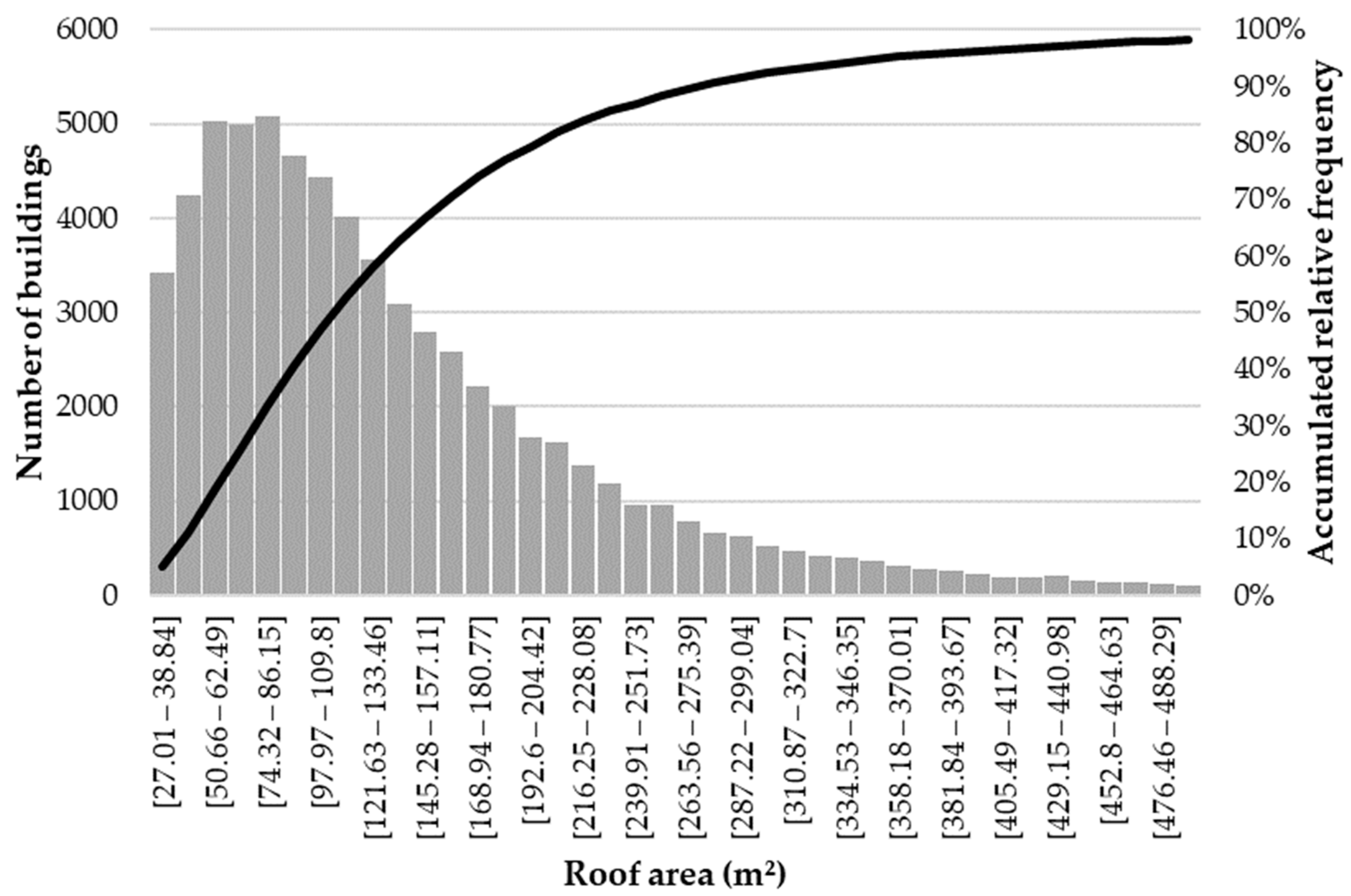
Next, a frequency distribution analysis of the group of houses and subgroups of flats according to the building roof area was carried out, establishing roof-size categories. The number of categories was defined through statistic formulas [
35], which were based on the number of buildings in each group. For the group of houses, the number of categories into which the group was divided was determined according to Rice’s formula, which is an alternative to Sturges formula, using Equation (1) [
36].
where
The group of houses was then divided into k categories with equal intervals. For each category, a representative building was chosen, corresponding to all buildings within its interval, with its roof area being the average of the roof area of all real buildings in the interval.
For flats, each subgroup was divided into categories according to the square root formula, using Equation (2) [
35].
where
In this case, the categories were divided into non-equal intervals according to the natural breaks method, which seeks to minimise variance within categories and maximise differences between them. For this, the Excel Real Statistics Resource Pack extension was used [
37]. A representative building was also chosen for each category, with a roof area equal to the average of all buildings in the interval. The choice of formulas was based on what seemed more suitable for each group given its number of buildings, so it would provide a satisfactory number of categories for use in simulations.
2.5. Rainwater HarvestingRainwater-harvesting Systems’ Simulation
The main components of rainwater harvestingrainwater-harvesting systems are the catchment area, which is usually the roof, water pipes and sometimes pumps, devices for disinfection, and storage tanks [
12]. The simulation of rainwater harvestingrainwater-harvesting systems was conducted using the
Netuno programme, which presents the results of the potential for potable waterpotable-water savings by using rainwater in relation to the storage- tank capacity. Its methodology is based on behavioural models, and all its equations can be found in [
23,
24,
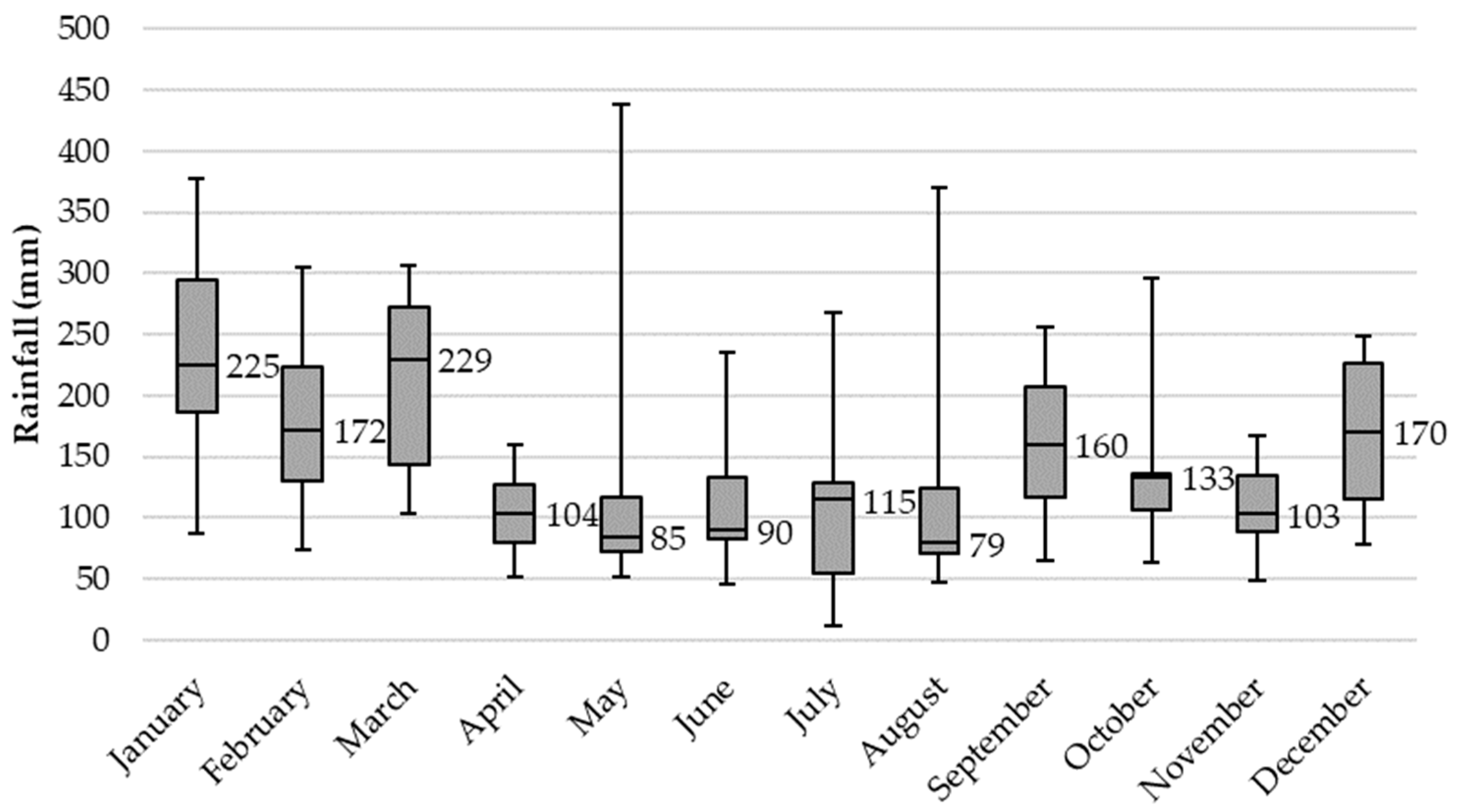
25]. The input parameters included daily rainfall data, the first flush, the catchment area, daily per capita water consumption, the number of residents, the rainwater demand, and the runoff coefficient. Daily rainfall data were obtained from the INMET website [
28]. The first flush was set at 2 mm, following the Brazilian standard for rainwater harvestingrainwater-harvesting systems [
38]. The catchment area was considered as to be the roof area of the representative building. The number of residents, daily per capita water consumption, and rainwater demand were considered according to each scenario. The runoff coefficient considered was 0.8, as it is the average value for ceramic- tile or fibre-cement roofs [
39].
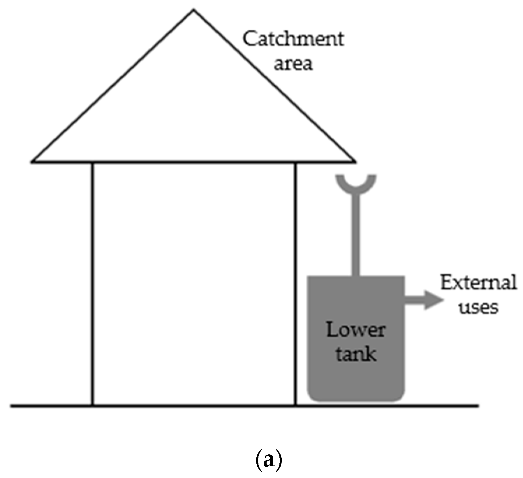
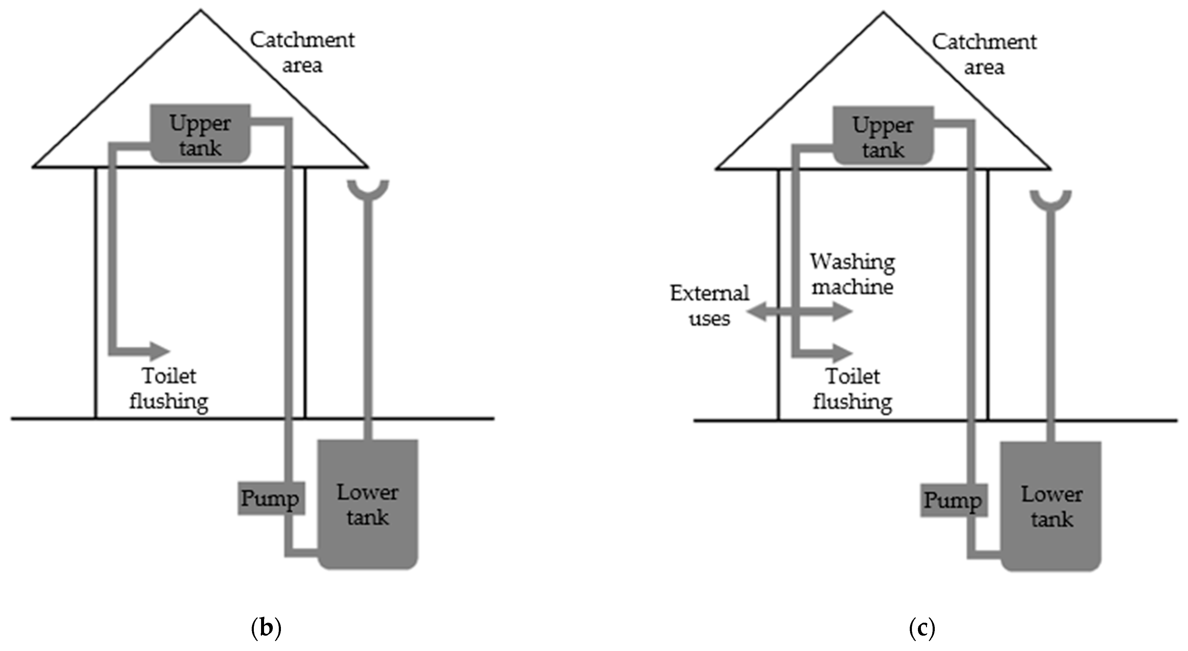
During the simulation, in order to determine the potable waterpotable-water savings, it was necessary to size measure the rainwater- storage tanks. For houses in scenarios with system design 1, only one lower tank defined by the programme was considered. For houses in scenarios with designs 2 and 3, and for flats in all scenarios, two tanks were considered: a larger lower tank that supplies an upper tank by means of a pump. In these cases, the capacity of the upper tank was considered to meet the daily rainwater demand of the building, while the size of the lower tank was defined according to the ideal capacity suggested by the programme.
Figure 3 shows the configuration of the system designs. In scenarios with system design 1, the lower tank was simulated for capacities between 100 and 5000 L for houses and 100 and 15,000 L for flats, both varying in intervals of 100 L. For scenarios with designs 2 and 3, capacities between 1000 and 15,000 L were simulated for houses and between 1000 and 60,000 L for flats, both varying in intervals of 1000 L. In all simulations, the ideal tank capacity was indicated when the difference in potable waterpotable-water savings was less than 1%/m
3 while varying the tank capacity.
As a result of the simulations, the potential for potable waterpotable-water savings of for each representative building for each scenario was obtained. This represents the percentage of potable water that can be replaced with rainwater. The size of the lower tank was also determined, being the capacity indicated as ideal by the Netuno programme.
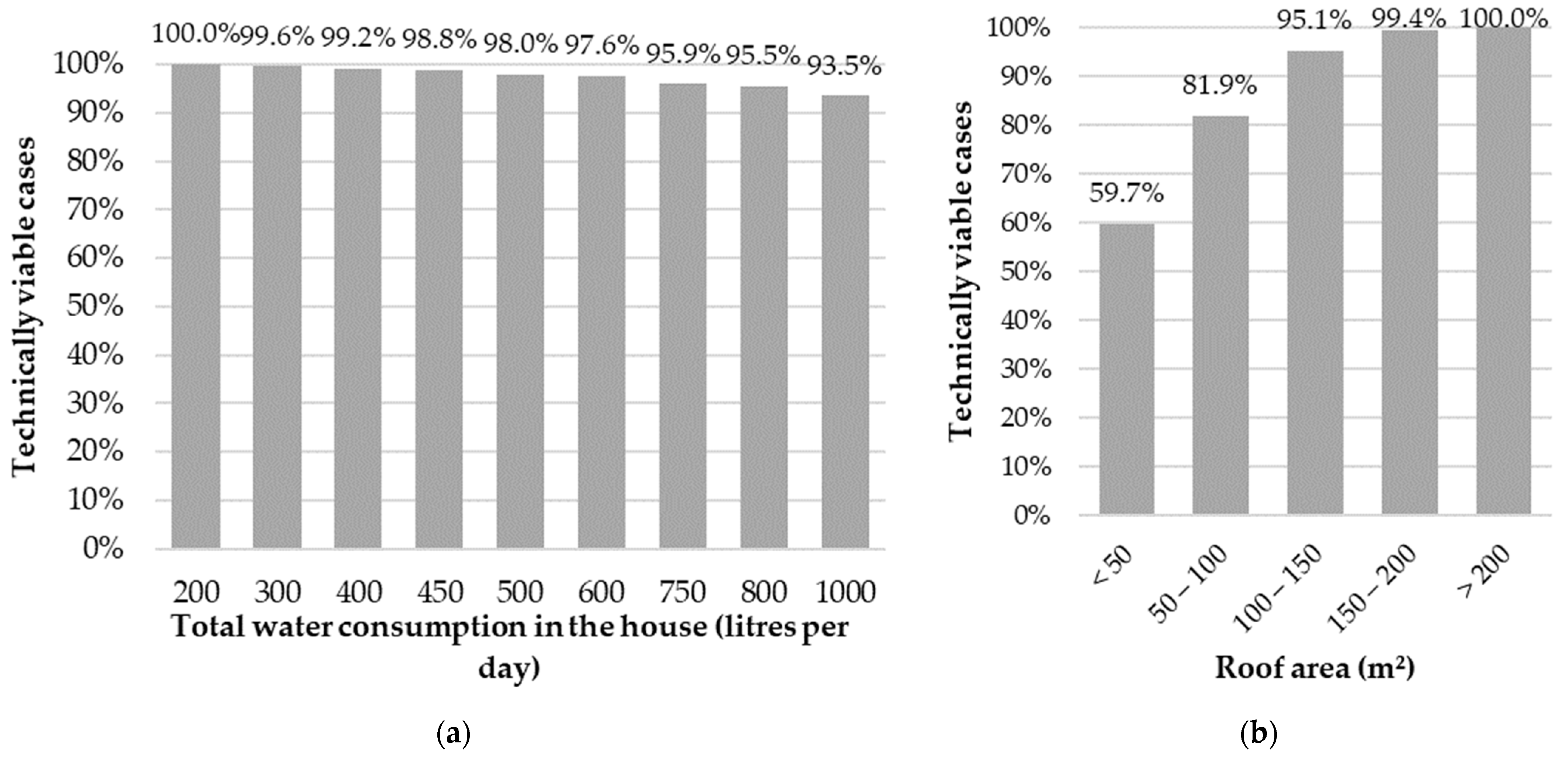
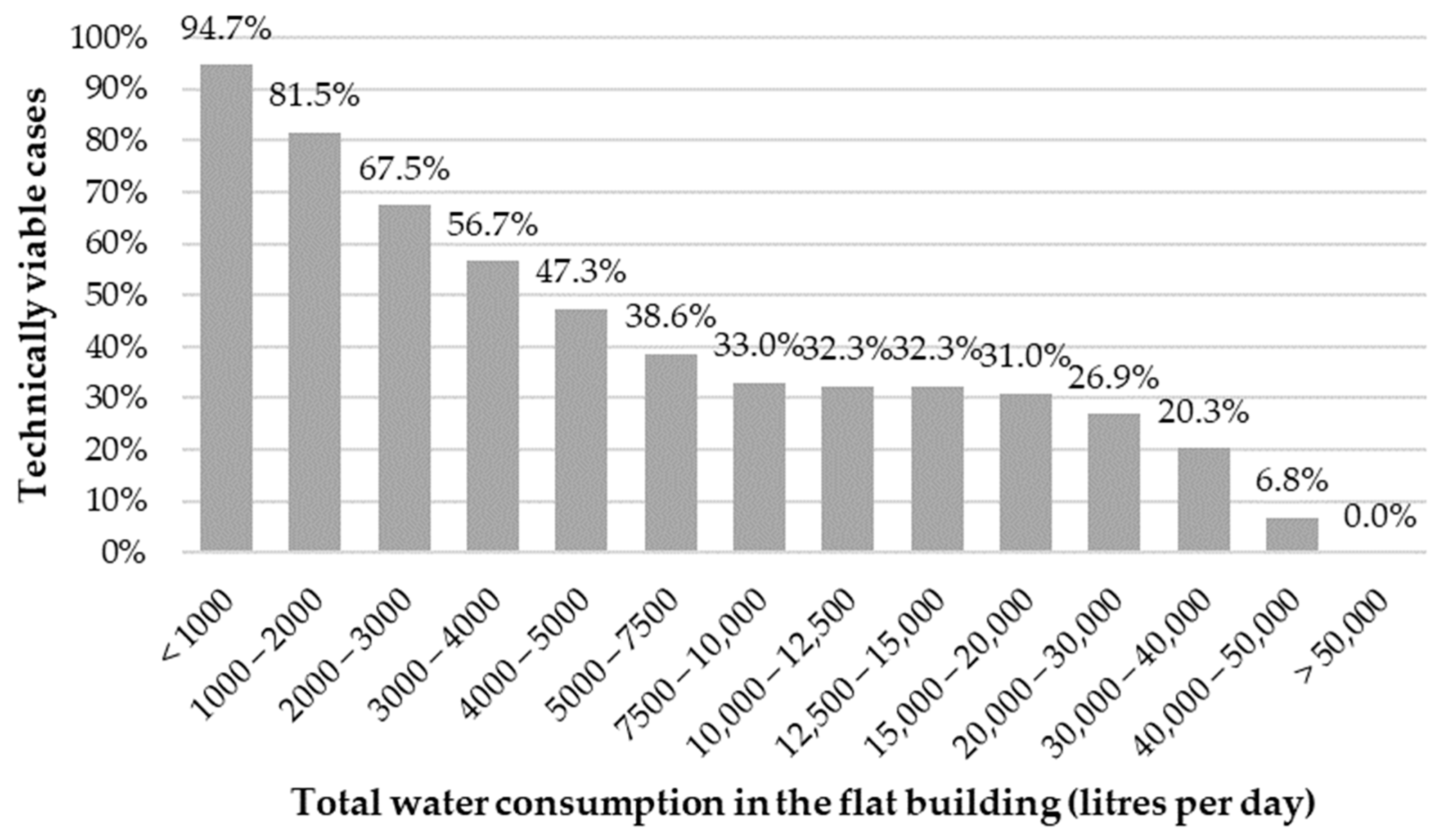
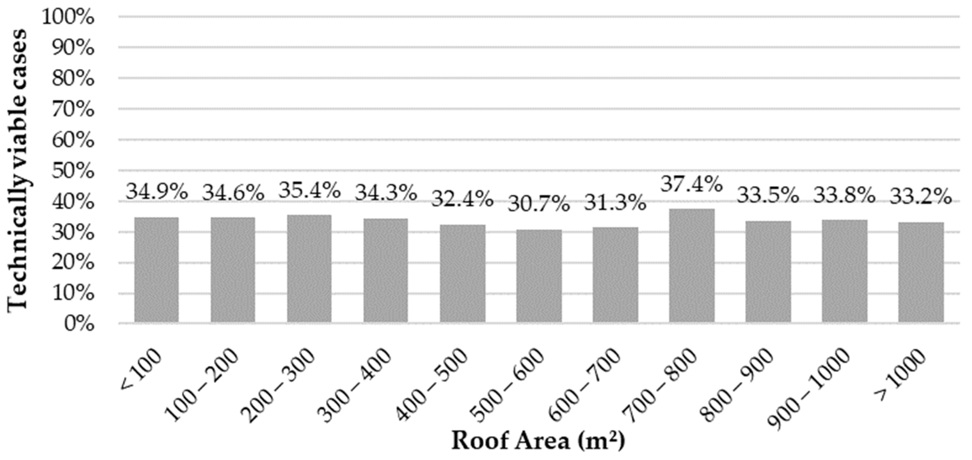
2.6. Technical Viability Assessment
From the results of the simulations, the technical viability of different system designs was analysed. The system was deemed technically viable when the potential for potable-water savings reached at least 90% of the rainwater demand of the system design. This was determined because if the system did not reach the designed rainwater demand, then a different design would be more suitable. Thus, cases that achieved the following were considered technically viable: 4.5% potential water savings for design 1, which aims to supply rainwater to meet the demand for cleaning activities and external uses, equivalent to a rainwater demand of 5% of the household water demand; 27% for design 2, to supply the demand for toilet flushing, equivalent to 30% of the household water demand; and 45% for design 3, to supply all non-potable activities in the dwelling, equivalent to 50% of the household water demand. The average potential for potable-water savings of the unviable cases was also assessed by calculating the arithmetic average of the potable-water savings of the cases that did not reach technical viability.
From the technical viability, a new parameter was formulated in order to analyse the catchment area necessary to collect one cubic metre of rainwater per month. Using Equation (3), the catchment area per cubic metre of rainwater was calculated for each simulation deemed technically viable. The roof area, the number of residents, and the total daily per capita water consumption are all input data of the simulation, while the potential for potable-water savings is the result of the simulation and already considers the rainfall, which is also an input parameter of the simulation. Thus, the minimum catchment area necessary to collect one cubic metre of rainwater per month in the city was considered to be the smallest value obtained for this parameter among the technically viable simulations. This parameter is exclusively related to the specific situation of the city and the data used in the simulations.
where
is the catchment area per cubic metre of rainwater (m2/m3);
is the roof area of the representative building simulated (m2);
is the number of residents in the scenario simulated;
is the total daily per capita water consumption in the scenario simulated (litres);
is the potential for potable-water savings (%).
2.7. Economic Feasibility Assessment
The economic feasibility analysis was conducted using an Excel spreadsheet. Costs were estimated for both the installation of the rainwater-harvesting system, referred to as initial costs, and the expenses associated with its operation, the operational costs. Both costs were calculated individually for each simulated system, as they differ depending on the model, the tank capacity, and the water-consumption results.
The initial costs included expenses on materials and labour. The materials considered were the lower and upper tanks, which were polyethylene water tanks, the pump, and other accessories such as PVC pipes, excluding gutters. Pumps were not accounted for in the simulations of houses under scenarios with system design 1, as this design does not require water pumping since it only has a lower tank. Material prices were determined through market research from local stores and suppliers, and labour costs were obtained from the National System of Costs and Construction Indexes (SINAPI) for October 2021 in the state of Santa Catarina. As accessories’ costs depend on the system design, it was estimated that these components represent 15% of the initial cost, i.e., the cost of tanks, pump, and labour, as in [
8].
Operational costs included energy for the pump operation, supplies for water treatment, and system maintenance. Chlorine tablets were considered to be part of water treatment, with the cost per cubic meter of treated water being obtained through local store research. The annual maintenance cost for the system was estimated at 1% of the initial cost, as in [
40], and is meant to account for any repair needed for the system. The operation energy cost was obtained from the pump characteristics, the monthly pumped water volume, and the energy tariff price. The energy tariff price with taxes applied was obtained from the website of the local energy supplier for December 2021 [
41]. The water volume pumped is equivalent to the system’s monthly rainwater consumption.
On the other hand, the economic benefit was obtained by means of the reduction in the water and sewage bill resulting from potable-water savings. Based on the daily per capita water consumption and the number of residents per dwelling in each scenario, the total water consumption for the dwelling was calculated over a month by multiplying such values by 30 days. Thus, the water and sewage bill without the rainwater-harvesting system was calculated based on the tariff prices and the monthly total water consumption for the dwelling. Subsequently, the monthly potable-water savings by the system was subtracted from the monthly total water consumption, and the water and sewage bill was recalculated. The difference in the bills with and without the rainwater-harvesting system resulted in the monthly monetary savings.
Analyses were conducted considering both the former water-tariff format and the current one to compare whether the system’s viability is altered and which one brings more benefits to users. The former tariff format charged a minimum fee for consumption up to 10 m
3, beyond which the amount was charged per each m
3 of water consumed, varying in consumption intervals. The current tariff format, implemented in 2020, no longer has a minimum consumption, charging a fixed fee for infrastructure availability and fees per m
3 of water consumed, also varying in intervals. Tariff values for 2019, representing the former tariff format, and 2021, the current one, were used. These values were obtained from the water company’s website [
42].
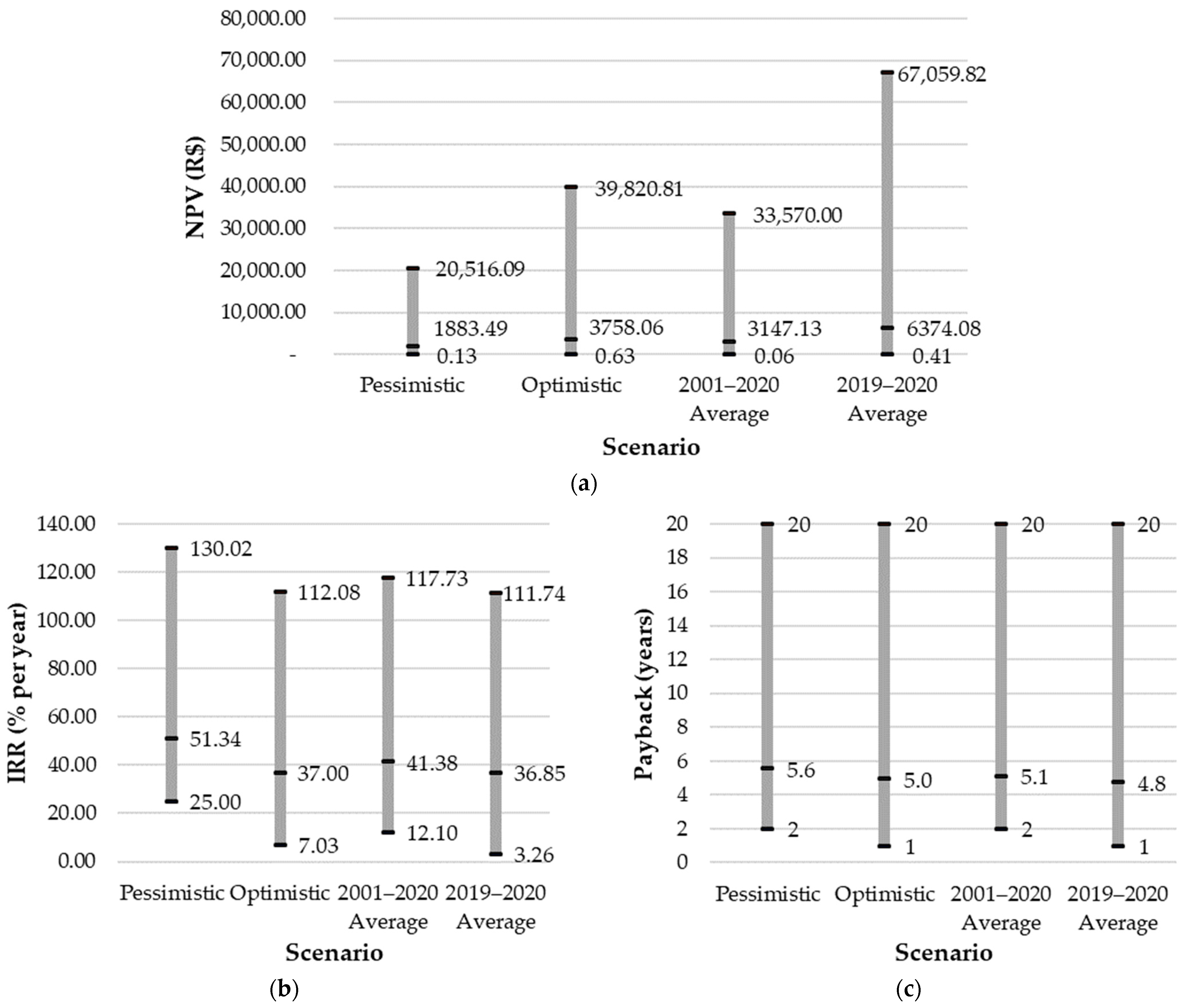
An annual cash flow was formed for a twenty-year period, as in [
8], and the discounted payback, internal rate of return (IRR), and net present value (NPV) were used as feasibility indicators. These indicators were calculated using the corresponding functions in the Excel spreadsheet, which are based on Equation (4) [
43]. Both the IRR and discounted payback are obtained based on the NPV, i.e., the IRR is the rate of return in which the NPV equation is equal to zero, and the discounted payback is the year of the cashflow in which the NPV becomes positive.
where
is the net present value (R$);
is the total period of the investment (years);
is the year of the cashflow (years);
is the cash flow for the tth period (R$);
is the rate of return (%).
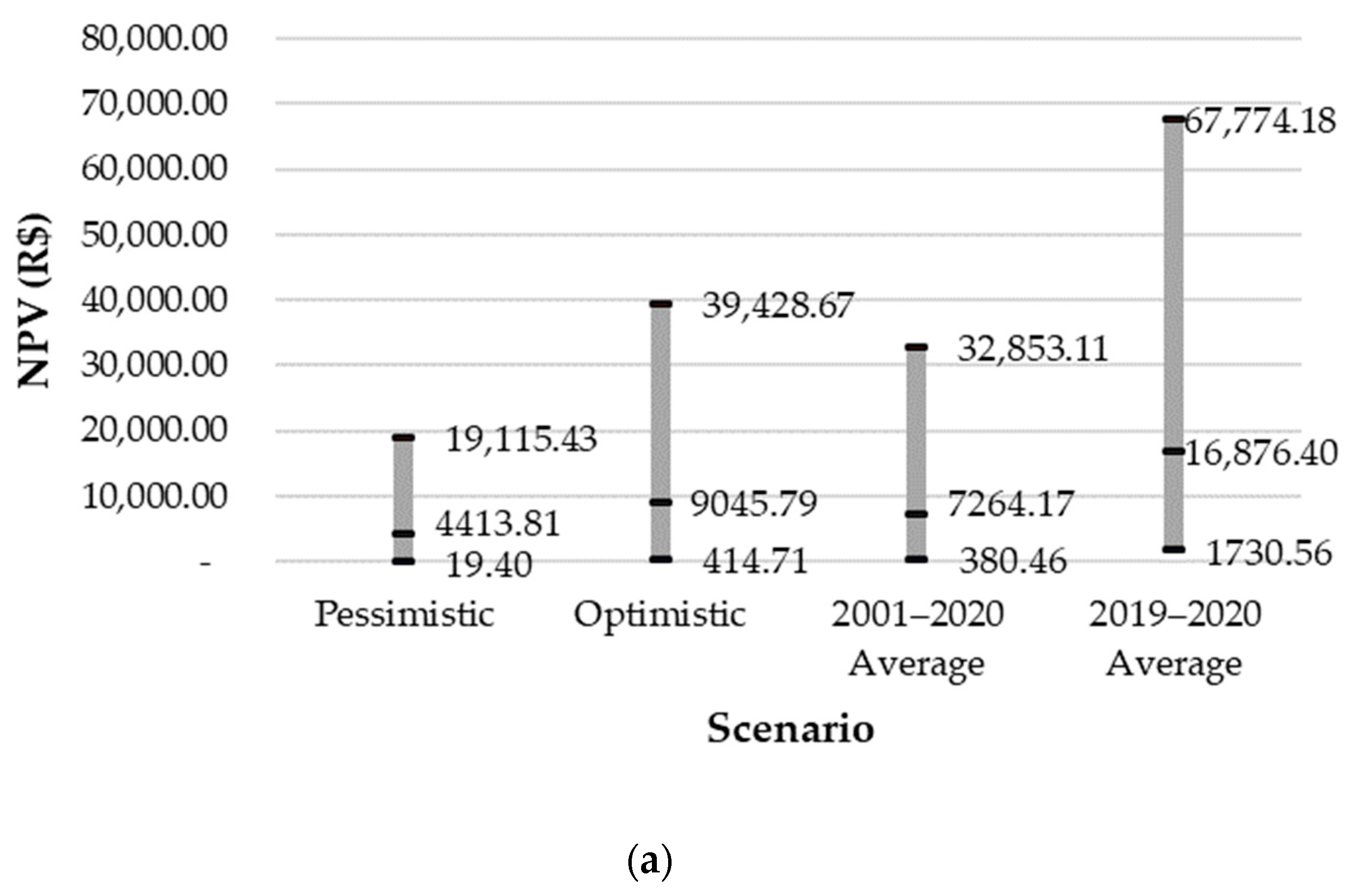
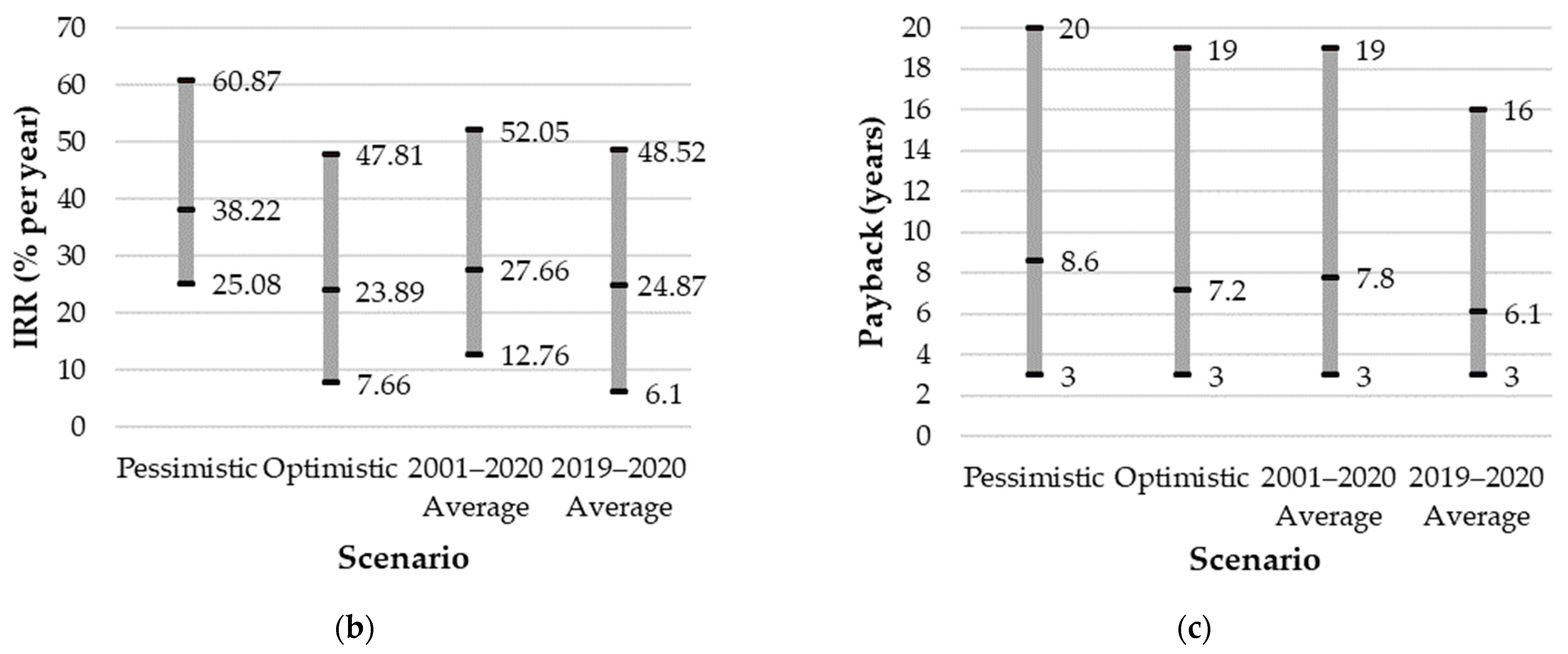
For the cash flows, a minimum attractive rate of return (MARR) was considered and the water and electricity tariffs were adjusted every year according to the inflation. The inflation used was the Broad Consumer Price Index (IPCA), which is the official government index, and the MARR considered was the Selic index, on which the interest rates of savings accounts in Brazil are based. Four different economic scenarios were evaluated: one pessimistic, one optimistic, and two averages. The pessimistic scenario considered the highest inflation of the last twenty years, and the optimistic scenario the lowest, alongside the Selic index of the same year. One of the average scenarios, called the 2001–2020 average scenario, considered the average inflation and Selic of the last twenty years, while the other, called the 2019–2020 average scenario, considered the averages only of the last two available years. For this, the IPCA and Selic index were obtained from the Central Bank website [
44,
45]. As the Selic varies throughout the months, the value considered was the one valid on December 31 of each year.
Table 1 shows the scenarios evaluated. The pessimistic scenario occurred in 2002, and the optimistic one in 2017; the 2001–2020 average considered values between 2001 and 2020, and the 2019–2020 average considered values from 2019 and 2020. To compare tariff formats, only the 2019–2020 average scenario was used.
The economic analysis was conducted for each case simulated. For the flat group, despite simulations being performed as collective systems and considering water consumption for the entire building, the economic analysis was carried out for each flat. Therefore, individual water bills were considered, with the average water consumption for the building, and the initial and operational system costs were divided among the flats in the building. Finally, the economic feasibility of each case was examined. The investment was considered economically feasible when the discounted payback was less than the analysis period, the NPV was positive, and the IRR was greater than the MARR.


