Abstract
The process of estimating sediment load has been a daunting issue in hydraulics and the water resource field. Several methods exist for predicting the sediment load in a catchment or river, but the majority of these methods are empirical and depend on the specific location where they are used. Understanding the underlying mechanism of sediment generation and its transport in connection with precipitation, topography, and subsurface conditions to characterize its process is helpful for determining the sediment load in a river. For this purpose, we analyzed the daily suspended sediment data measured for 8 years at the headworks of the Kabeli A hydropower project in the Kabeli River, which originates from the Himalayan region. The analyses show that the suspended sediment concentration (SSC) varies in an orderly manner over time and asynchronously between seasons with respect to the river discharge. Clockwise hysteresis is observed in the yearly plots between the SSC and river discharge. The hysteresis becomes narrower when compared with the direct runoff obtained from a digital filtering algorithm and, even more so with the direct runoff from the hydrological model SWAT. The analysis shows that the sediment concentration is controlled not only by the total discharge in the river but also by the contribution of ground water to the river discharge, indicating that the total discharge alone cannot reflect the seasonal variation in SSC. It is inferred that the river is supply-limited and the hillslope is transport-limited with respect to sediment sources. The SWAT model suggests that the base flow contribution to the total river discharge is 78%. Here, we present a method for constructing the suspended sediment rating curve by comparing the direct runoff with the sediment concentration. The deduced sediment rating curve captures 84.51% of the total sediment load over the study period in the Kabeli River. This method may potentially be used in similar catchments with supply-limited rivers and transport-limited hillslopes.
1. Introduction
The Himalayan region is the source of perennial rivers and is known for its abundant water resource potential but with rugged and steep topography. The region has among the highest sediment yield rates in the world [1,2]. Rivers originating from the Himalayan region are steep to very steep and transport a considerable amount of sediment, with a high degree of seasonal variability due to the monsoon-dominant climate. High tectonic activity, rapid weathering, and steep topography influence the rate of sediment yield to the river network. The monsoon season accounts for about 80% of the annual precipitation. During this period, intense rainfall occurs, causing sheet erosion and mass wasting/landslides, which is very common in the catchment with steep terrain, producing a lot of sediment [3]. As a result, up to 98% of the annual sediment load is transported during the monsoon period [4].
The quantification of sediment yield is necessary for the sediment management of water resource projects, like hydropower. The data on long-term suspended sediment loads (SSLs) around the world, especially in the Himalayan region, are scarce [5]. Multiple years of fragmented sediment data are available; however, they are mostly related to the outlets of major river basins in flatter downstream areas. These data may not be representative of the tributary rivers located at the highland regions with much steeper gradients. Most of the hydropower project sites are located in the upper catchments of the major rivers and in their tributaries where the sediment source and transport mechanisms are different than the flatter downstream areas. Hence, the lack of long-term monitored data has constrained the understanding of the sediment discharge pattern in the upper catchment of the major river systems and their tributaries with steeper gradients.
Several attempts have been made in estimating sediment yield using various approaches that involve the comparison of the morphometric parameters of a catchment to relate sediment yield [6]. Others utilize distributed and lumped models that relate catchment and climatic variability to estimate the lumped sediment yield values [7,8,9]. Despite the availability of these methods, it is still a challenge to predict the sediment load. Suspended sediments are widely used as a primary proxy for predicting the sediment load in a river [10]. The intermittent SSC can be linked with discharge data using a rating curve to estimate the SSC from the river discharge. Some of the methods to derive the suspended sediment rating curve are the ordinary least square (OLS), Ferguson method [11], Duan unbiased method [12], and optimization method [13]. The rating curve methods do not refine the parameters physically but rather involve statistical improvement, either by bias correction or an equivalency approach [5]. The estimation of the sediment load using the total discharge is not straightforward. The interpretation of suspended sediment measurement data requires the process of differentiation between the conditions of sediment transport and supply limitation [14].
The distinction between supply-limited and transport-limited systems is important to understand the mechanisms of the sediment transport process. In an incised, erosional, and steep river, the streamflow increases the sediment transport capacity of the river. At some point, at sufficiently large discharge, the sediment in the river gets exhausted. This causes the flattening of the sediment vs. discharge curve (Figure 1a) and the maximum value of the sediment concentration is referred to as the ultimate sediment concentration [15]. In a hillslope/catchment with a sufficient amount of available erodable material, the sediment supply is greater than the transport. However, at very high precipitation, the supply gets exhausted. In this condition, the river receives constant sediment from the hillslope as shown in Figure 1b.
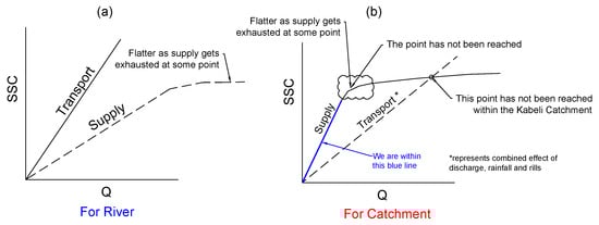
Figure 1.
Suspended sediment yield status of the Kabeli River and its catchment. (a) Sediment transport process for the river. (b) Sediment transport process for the catchment (hillslope).
Sediment studies involve identifying the bedload and suspended loads to calculate the total sediment load in a river. In some rivers, the bedload accounts for a large fraction of the total sediment load. It is regarded as the most difficult fluvial process to interpret and measure [16]. A study in the Narayani Basin suggests that due to technical difficulties in measurements, the available data were too scarce to interpret the exact concentration of the bedload [17]. In high mountains, the bedload comprises about 30% of the total sediment load [10]. Unlike the general suggested values of the fraction of the bedload of about 2% to 12% by Land and Borland, 1951 [18], the study of the Marshyangdi River shows that the bedload accounts for ∼35% of the total sediment load [19]. Another work by Attal and Lavé, 2006 [20], shows that the fraction of the bedload is about 12% to 18% for the major rivers at outlets of the Himalayan range. According to Andermann et al., 2012 [21], significant bedload movements occur in the High Himalayas, while minor fractions occur in the Lesser Himalayas. This shows that bedload transport is largely variable and unknown, which is mainly due to difficulties in its long-term measurements.
According to Loyd et al., 2016 [22], a hysteresis analysis can be used to investigate and evaluate sediment movement in relation to streamflow during certain hydrologic events. In sediment studies, hysteresis is the lag or lead that is seen in the sediment concentration with respect to the discharge or streamflow. Hysteresis is ascribed to different factors that control the supply and transport of sediment, namely, the magnitude and sequence of flood events, sediment particle size distribution, basin size, land use and sources of sediments, and so forth [23]. Event-wise hysteresis is mostly described in the literature where the timing of flood events dictates the type of hysteresis [24]. According to Misset et al., 2018 [25], event-wise counterclockwise hysteresis behavior is observed if the sediment sources are distant, clockwise hysteresis is observed if the sediment sources are proximal, and no hysteresis is observed if there is an unlimited sediment supply. An event-based analysis can be performed where the frequency of the sediment concentration and discharge sampling is high. Most of the hysteresis is observed due to the unavailability of sediment, i.e., sediment exhaustion where the source (particularly the catchment and sometimes in-stream) cannot deliver sediment to the river [23].
An annual-scale clockwise hysteresis was revealed by an extensive data analysis [21] in the Karnali, Narayani, and Saptakoshi basins in Nepal. Similarly, Chhetri et al., 2016 [26], also observed clockwise hysteresis behavior in the Langtang River where the sediment concentration is higher in the pre-monsoon season relative to the post-monsoon season for the same discharges. Similar seasonal hysteresis behavior is also observed in the sediment load and discharge rating curves in the glaciarized catchments in Nar Khola in the Marshyangdi Basin by Gabet et al., 2008 [27], and even further to the west in the region of Garhwal Himalaya in India [28]. Gabet et al., 2008, and Hasnain and Thayyen, 1999 [27,28], ascribed hysteresis to the decrease in glacier-derived sediments during the summer melt season. In contrast, Morin et al., 2018 [17], analyzed data from the Narayani River for one year and regarded the dilution of landslide-derived sediments by the base flow fraction of ground water as the supporting cause for clockwise hysteresis. Andermann et al., 2012 [21], also referred to the ground water contribution as the cause of hysteresis in the major river basins of Nepal.
The aim of this manuscript is to focus on the seasonal hysteresis behavior rather than event-wise hysteresis. The frequency of observed data is not sufficient to study the event-scale hysteresis behavior. Hence, the main emphasis is to find the seasonal linearity in the sediment and discharge relationship. The understanding of the seasonality of sediment is based on the study of seasonal trends of sediment transport in the river and the characterization of the underlying mechanism of suspended sediment in relation to discharge hysteresis phenomena. The goal is to better understand the source and transport mechanisms of sediment in relation to precipitation and topography and to determine the runoff and ground water component of river discharge that could potentially help to improve the suspended sediment rating curve.
2. Study Area
The study area is located in the eastern part of Nepal in the Kabeli River, which originates from the Himalaya and drains following rugged terrain and a steep valley to meet the Tamor River–a major tributary of the Saptakoshi River. The Kabeli Basin is located in between latitudes 27°13′ and 27°32′ N and longitudes 87°43′ and 88°04′ E. The catchment of the Kabeli River is selected for this research considering the availability of the fairly long-term discharge and suspended sediment data of the river. Additionally, the river is perennial and its catchment expands across four physiographic zones according to LRMP 1986 [29].
The catchment area of the Kabeli River is 862 km2 at the intake location of Kabeli hydropower, where a streamflow and sediment sampling station are setup. The catchment elevation ranges from 560 to 5487 masl with a mean elevation of 2427 masl. The catchment area above the permanent snow line (5000 masl) is only about 1 km2. The river gradient is relatively steep and flows through the valley sides with a steep terrain where about 60% of the catchment has a gradient larger than 50%. The location map of the study area is shown in Figure 2.
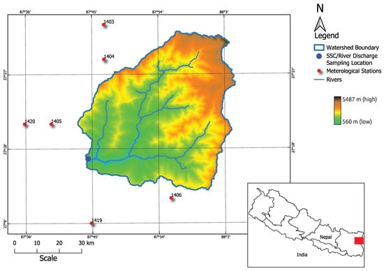
Figure 2.
Location map of study area.
Like other rivers of the Himalaya, the Kabeli River has variable annual flow patterns due to the variability in precipitation, as well as topographic and geological characteristics. The season can be divided into four categories, namely, winter (December–February), pre-monsoon (March–May), monsoon (June–September), and post-monsoon (October–November). The monsoon rainfall accounts for 76% of the mean annual rainfall of 2022 mm, whereas only 54% of the total river flow occurs in the monsoon season. This high variability in precipitation controls the whole environment of the catchment, consisting of vegetation, land cover, landslide susceptibility, water availability, sediment erosion, etc.
3. Data
For the development of the Kabeli ‘A’ Hydroelectric Project (37.6 MW), Kabeli Energy Limited conducted suspended sediment and flow sampling from 2010 to 2018. The river discharge was recorded from May 2010 to January 2018. Similarly, the sediment data were also measured twice a day with additional measurements during the heavy sediment influx days of the pre-monsoon and monsoon seasons [5]. A summary of the observed sediment and river discharge data is given in Table 1.

Table 1.
Summary of observed suspended sediment concentration and flow data at Kabeli intake site (for 4572 data points).
The data from six ground-based meteorological stations obtained from the DHM were used in this study. The precipitation data were collected from all the weather stations (1403, 1404, 1405, 1419, and 1420) as indicated in Figure 2, whereas the temperature and humidity data were collected from station nos. 1405 and 1419. The sunshine hours and wind speed were taken from station no. 1405. The details of the data resolutions and sources are given in Table 2.
Table 2.
Data types, their sources, and resolutions.
Missing precipitation data in the ground-based station were filled with the APHRODITE (Asian Precipitation Highly Resolved Observational Data Integration towards Evaluation of Water Resources) dataset available at (http://www.chikyu.ac.jp/precip/ (accessed on 14 December 2020)) with the daily version for monsoon Asia (APHRO_MA_V1101EX_R1) having a spatial resolution of 0.25° (∼30 km) with linear scaling or transformation at each gauged station. This is the best satellite dataset available for the whole of Nepal, calibrated with ground-based data [30]. The Thiessen polygon method was used to calculate the basin average daily precipitation values. Figure 3 illustrates the daily observed precipitation, river discharge, and sediment concentrations.
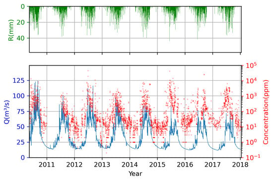
Figure 3.
Eight-year (2010–2018) temporal variability in precipitation, discharge, and sediment concentration. Daily precipitation hyetograph (green), daily river discharge hydrograph (blue), and SSC (red with scatter plot). The sediment concentration is on a logarithmic scale. Missing ground-based precipitation data were filled with the APHRODITE dataset (APHRO_MA_V1101EX_R1). Basin average daily precipitation values were calculated using Thiessen polygon method.
4. Research Methodology
The research methodology adopted comprises the process of determining an accurate estimation of base flow to derive direct runoff and comparing it with the sediment concentration and sediment load, as depicted in Figure 4. It is to be noted that the general setting of sediment source and transport phenomena are intertwined with precipitation cycles in the Kabeli Basin. Hence, a hydrological model, Soil and Water Assessment Tool (SWAT), is used to determine improved base flow and direct runoff. The analysis was useful to evaluate the sediment source and transport mechanism, thereby helping to deduce a method for constructing a suspended sediment rating curve from a direct runoff approach.
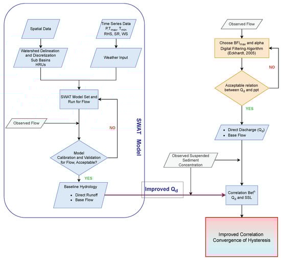
Figure 4.
Methodology adopted for this study.
4.1. Flow Separation Using Digital Filtering Method
The total discharge of the river comprises two components consisting of the direct runoff and base flow. Base flow is the discharge generated by precipitation after it has passed through certain geological features of the catchment that responds slowly to rainfall events. Direct runoff is the fast component of the total discharge that generally occurs with precipitation. In this study, direct runoff is defined as the fraction of the total river discharge with a short response time of less than a day. The separation of the base flow from the total runoff is useful for determining the direct runoff in the river. In some rivers of Nepal, direct runoff only accounts for about 20% of the annual river discharge [31] but contributes significantly to the flow of sediment from the basins [21].
The direct runoff that is the product of effective rainfall [32], in general contributes to surface erosion in the catchment and may be directly linked to the sediment concentration or sediment load in the river. This approach is inferred to be logical, as it relates to the real cause and its effect rather than comparing the concentration with the total discharge. So, the authors have focused on the direct runoff, potentially narrowing down the hysteresis loop in the sediment vs. discharge relationship while maintaining physical rationality in the process.
It is believed that the hysteresis phenomenon may be addressed in a rating curve when the real cause of the sediment flux, i.e., direct runoff, is considered instead of the total discharge. With this in mind, the authors reviewed the different methods available for obtaining the base flow of a river from the total river discharge. Some of the widely used digital filter methods are Eckhardt [33], Arnold and Allen [34], Gupta [35], the web base WHAT [36], etc.
The separation was performed with the two-parameter digital filtering algorithm suggested by Eckhardt, 2005 [33], which is widely used due to its simplicity. This method has also been used in flow separation in different river basins of Nepal by Andermann et al., 2012, and Morin et al., 2018 [17,21]. The method filters highly unusual signals (direct runoff) with low signals (base flow) via an electrical analogy as shown in Figure 5a.
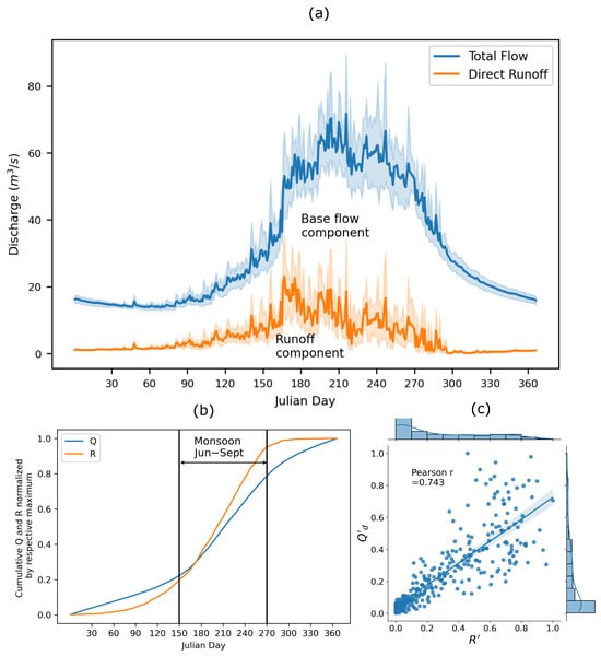
Figure 5.
The average yearly hydro-climatological condition depicted at the hydrological station in the Kabeli Basin (∼8 yr). (a) A discharge hydrograph of the Kabeli River. The runoff component is the average daily discharge contributed by the direct runoff, . The base flow represents the slow flow component. The hydrographs are separated using two-parameter filtering methods suggested by Eckhardt, 2005 [33]. (b) A cumulative representation of the mean basin precipitation R and river discharge Q (normalized by their respective maximum values), showing the temporal phase shift. (c) A plot displaying the relationship between R and , indicating the dependency of on R (both normalized with their respective maximum values). The faint hatch in the above figures shows 95% confidence intervals.
The filter parameter is not as sensitive as the maximum base flow index to the calculated mean base flow. Eckhardt, 2005 [33], estimated representative values for different types of hydrological and hydrogeological catchments. The can be taken as 0.8 for perennial streams with porous aquifers, 0.5 for ephemeral streams with porous aquifers, and 0.25 for perennial streams with hard rock aquifers. Andermann et al., 2012 [31], adopted as 0.98 and as 0.8 for all the considered rivers in Nepal, whereas Morin et al., 2018 [17], set the to 0.75 and the values of between 0.91 and 0.987 for high and low base flows, respectively.
The parameters of Eckhardt, 2005 [33], were calibrated by determining the maximum linearity (coefficient of correlation) between the daily values of rainfall and direct runoff, which is rational because rainfall is the direct cause of direct runoff. It should be noted that the time of concentration for the Kabeli catchment is 3.5 h, and the effect of the rainfall is observed at the outlet on the same day. The was calibrated around a recommended value of 0.8 to determine the maximum Pearson coefficient r and with an of 0.98. The was not as sensitive as the . This process was continued until the value converges, which resulted in the of 0.73 and of 0.98. The rainfall pattern and direct runoff agree with the pattern and are closely related with a coefficient of regression of 0.743 as indicated in Figure 5c. The separated flows from 2010 to 2018 in the Kabeli River are shown in Figure 5a. The estimation of the parameters for this method is based on the rainfall in the catchment (Figure 5c), which is more sensitive to measured precipitation. It is to be noted that there are no rainfall gauge stations within the catchment area, which might cause the estimated parameters to deviate from their actual values. Moreover, the rainfall stations are located at lower elevations, which may introduce uncertainty when calculating the average daily basin precipitation values. The scattering of and R could be due to the lack of localized rainfall data.
4.2. Flow Separation Using the SWAT Model
To determine the contribution of the base flow to the total discharge in the Kabeli River, the water balance was assessed at the catchment scale using the SWAT model. SWAT’s ability to estimate hydrology is notable, and it is believed that the process-based model can predict the base flow and direct runoff more precisely than digital filtering algorithms. SWAT incorporates multiple input data and parameter calibration. It is also well known for its comprehensiveness and ability to simulate flow in various types of catchments [37]. Therefore, the SWAT model was chosen to separate the flow.
The is influential parameter in determining the base flow in the SWAT model. However, there are other parameters that also govern the base flow in addition to the because of their interaction in the model [38]. The hydrological model was set up with calibration and validation, which was performed by adjusting the sensitive parameters. Minimizing the difference between the observed and simulated streamflows is an important goal of calibration. Subsequently, the model was validated by examining the parameters with a whole set of new data from subsequent years. The results of the calibration and validation are shown in Figure 6.
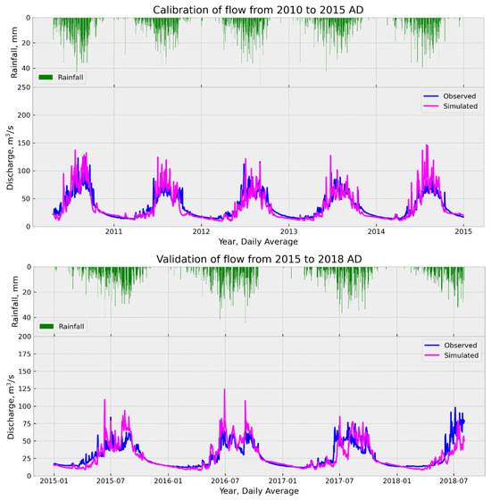
Figure 6.
Calibration and validation of streamflow from SWAT model.
The simulation statistics revealed that the model performed well during the calibration period for the streamflow. The Nash-Sutcliffe efficiency (NSE) obtained was 0.75, obtained was 0.75, and percentage bias (PBIAS) obtained was 1.87%. The performance evaluation criteria suggest that the model is deemed ‘good’ in terms of the streamflow calibration at the watershed scale. The model performed on average during the validation period for the flow. The NSE was 0.57, the was 0.66, and the PBIAS was −8.5%. The inconsistency in the measurements and the lack of recalibration of the rating curve for the discharge measurements in later years may be the cause behind the lower NSE values in the validation period. The performance evaluation criteria suggest that the model is deemed ‘satisfactory’ in the validation of the streamflow at the watershed scale. The calibration and validation performance evaluation criteria were set according to Moriasi et al., 2007 and 2015 [39,40].
5. Results and Discussion
5.1. Hysteresis Loop
When the observed sediment concentration is compared with the streamflow by color coding the months, as shown in Figure 7 (bottom right), there are two sediment concentration ranges for the same river discharge. It is evident from the figures that the sediment concentration is higher in the pre-monsoon season than in the post-monsoon season for the same magnitude of discharge. Similarly, the pattern of the sediment concentration shows similar behavior throughout the years as illustrated in Figure 7. This implies that, in the Kabeli River, the sediment concentration varies asynchronously with the total discharge and shows systematic clockwise hysteresis behavior on a yearly scale when plotted against the total discharge.
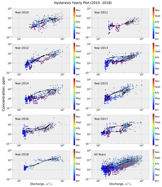
Figure 7.
The suspended sediment concentration and streamflow of each year of the study period. The monthly average sediment concentration and discharge are plotted for each year from 2010 to 2018. The figure in the bottom right represents the same for all years. The color marker is adjusted according to the calendar age (1 = January, 12 = December). The black arrow lines represent the monthly mean values of the SSC and Q. Clockwise hysteresis is evident in all years when a full dataset is available.
However, separating the base flow from the total streamflow and comparing the concentration with that of the direct runoff revealed different characteristics of the plots. When the sediment concentration is plotted against the direct runoff, the hysteresis behavior of the SSC narrows down (Figure 8).
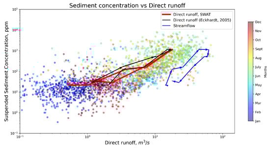
Figure 8.
Bi−logarithmic plots of the SSC vs. direct runoff of the total river discharge Q for the Kabeli catchment over the study period (∼8 yr). The color marker is adjusted according to the calendar age (1 = January, 12 = December). The black arrow lines represent the monthly mean values of the SSC and from Eckhardt, 2005 [33], and the red arrow lines represent the monthly mean values of the SSC and from the SWAT output, whereas the blue arrow lines represent the monthly mean values of the SSC and Q.
Most studies have concluded that clockwise hysteresis is due to the exhaustion of the sediment that is available to be transported by the stream [23]. However, this explanation does not seem to hold true in the case of the Kabeli Basin. The dependency of the sediment concentration on the direct runoff appears to be the driving factor behind the observed hysteresis phenomenon (Figure 8). Around 76% of the rainfall and 54% of the total annual flow occurs in the monsoon season. The rate of accumulation of the rainfall increases more in the pre-monsoon season (March–May) than the total discharge Q (Figure 5b). As the rainfall R is related to the direct runoff (Figure 5c), more rainfall would increase the in the river flow and hence increase the sediment concentration.
Similarly, the accumulation of the rainfall stops at and beyond the post-monsoon season (October–November), but the cumulative values of the discharge are continuous due to the ground water flow (base flow). During this period, in-stream erosion is the major factor for the SSC in the river. This implies that ground water is among the contributing factors of streamflow after the post-monsoon season. As the ground water from the watershed does not generate or transport sediments to the river, this causes the dilution of the sediment in the river system. On the other hand, the sediment concentration is much higher in the pre-monsoon season than in the post-monsoon season for the same magnitude of discharge.
At a point at the start of the pre-monsoon season, the ground water storage is minimal due to the long dry season causing a minor contribution to the base flow of the total discharge in the river. Once the monsoon starts, the precipitation accounts for a major contribution to the river discharge during the monsoons. More importantly, higher monsoon precipitation contributes to more surface or direct runoff. The precipitation causes erosion in the catchment, which is the main source of sediment transport in the river system.
By the end of the monsoon period (post-monsoon season), the ground water storage is replenished by precipitation and is the main source of the river discharge. On the other hand, due to less surface runoff, the erosion in the catchment decreases considerably, leading to a substantial reduction in the suspended sediment flow in the river. This causes hysteresis in the plot between the sediment concentration and river discharge.
5.2. Base Flow from SWAT
The results of the analysis from the SWAT model show that approximately 78% of the total runoff accounts for the base flow, which agrees with the amount for perennial rivers of around 80% as mentioned by Eckhardt, 2005 [33]. It is also evident from the findings that (ground and soil water) accounts for approximately 80% of the total discharge in the Himalayan rivers [31].
A comparison of the total streamflow, the direct runoff obtained from the digital filtering algorithm, and the process-based output from SWAT with the SSC is shown in Figure 8. As evident from Figure 8, through visual judgment, the direct runoff from SWAT has made it possible to narrow the clockwise hysteresis, which partially resolved the seasonal dilution effect on the sediment concentration. The hysteresis of the sediment concentration decreased significantly, indicating that the direct runoff could be a better proxy that should be used for estimating the sediment concentration rather than the use of the total stream runoff in the Kabeli River. It should be noted here that the direct runoff contributes only ∼22% to the total annual flow.
5.3. Mechanism of Sediment Yield
The inflow of sediments over the period of study suggests that the sediment sources in the river catchment are not exhausted. The active monsoon and active tectonic activities create a conducive environment for the rock mass near the surface to weather quickly, converting the rock mass to fragmented rocks and granular soils along the topographic slopes (Figure 9), which are eroded and flushed by the monsoon rains. Moreover, mass movements are also triggered when the rainfall is intense. Notably, approximately 90% of sediment yield occurs during the monsoon season alone.
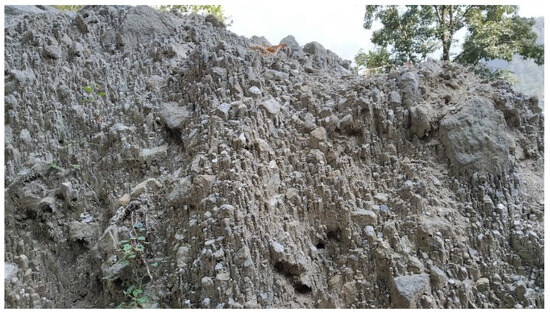
Figure 9.
Remnant of sheet erosion in fine-grained soils from similar physiographic regions near the study area (November 2020).
The ability of rivers to transport suspended sediments is dependent on the discharge, the intensity of the rainfall, and the river gradient [41]. The gradient of the Kabeli River is about 9°, which is regarded as a steep river, indicating a considerable capacity to transport the suspended sediment load downstream. The transport capacity of rivers in the high Himalayas and high mountains are always greater than the supply of sediments. In the case of the Kabeli River, the sediment concentration increases with respect to the river discharge without flattening (Figure 7). This indicates that there is no transition in the nature of the sediment transport in the river from a supply-limited to transport-limited condition. Therefore, sediment yield in the Kabeli River is supply-limited.
It is to be noted here that the supply of sediment from the catchment is dependent on the availability of erodible material on the hillslopes, the intensity of the rainfall, the surface runoff, and the magnitude of the fast component of the river discharge . As the river is supply-limited and the sediment in the river depends on the supply of sediment from the hillslope primarily induced by effective precipitation, which is related to , the catchment is transport-limited. Figure 1 illustrates sediment yield in the Kabeli River as well as from its catchment.
It is evident that the sediment concentration increased consistently with the sediment discharge in the Kabeli River [5]. Because the river catchment holds considerable weathered and fragmented material on the hillslopes, sediment yield will depend on the intensity of rainfall as indicated by the blue line in Figure 1b.
An example of a heavy rainfall event of 542 mm in a 24 h period in 1993 [42] caused a significant amount of sediment yield in Kulekhani Reservoir located at the central hills of Nepal. According to Shrestha, 2012 [43], about 19 million cubic meters of sediment (both suspended and bedload) were deposited in Kulekhani Reservoir within three monsoon seasons between the years 1993 and 1995. For a catchment area of 126 km2 and considering a bedload factor, packing factor, and specific gravity of 0.3, 0.8, and 2.64, respectively, for sediments, the specific suspended sediment yield from the catchment is calculated to be around 740 tons/hectare/year, which is considerably high compared to the observed 7.26 tons/hectare/year for the Kabeli catchment. This also suggests that the condition of the supply limitation of the sediment in the catchments of Nepal is beyond the present observation conditions.
5.4. Rating Curves from Direct Runoff
Various methods were used for the development of the suspended rating curves for the estimation of the suspended sediment load in the Kabeli river [5]. Among the adopted methods of the rating curve, the optimization method showed promising results in capturing the total sediment load over the study period but could not explain the yearly or seasonal variation. This study was based on a simple analysis without considering the seasonal variation in the sediment load that formed ladder-like patterns in cumulative plots without any intra-annual similarities in the observed and simulated load values.
Figure 8 shows that the direct runoff has a better relationship with the SSC in comparison to the total discharge in the river. When constructing rating curves, it is recommended to use the SSC instead of the SSL to minimize autocorrelation [5]. It is important to note that the SSC is measured alongside the total discharge Q and not with . The SSC reflects the sediment flux for the entire river discharge, not just the direct runoff. Therefore, comparing the SSC directly with can be misleading because represents only a fraction of Q. Consequently, when developing suspended rating curves from , it is advisable to use the SSL instead of the SSC.
Initially, a relationship was examined to determine if a power-law distribution exists between the direct runoff and sediment load. For this purpose, a maximum likelihood fit to the power-law distribution was applied to the sediment load as recommended by Alstott et al., 2014, and Gillespie, 2015 [44,45]. The Kolmogorov-Smirnov (KS) test for goodness-of-fit statistics is better for heavily tailed observations for validating power-law distributions [46]. Therefore, the heavy-tailed distribution was scaled to the point that resulted in a minimal KS distance between the data and the fit. The cutoff point used was 0.005 (Figure 10) and the number of samples is N = 1071∼1000. Taking the quantile value of the row of 1000 samples in Table 2 of Goldstein et al., 2004 [47], the KS distance equals to 0.0180, which is below 0.0186 (K statistics). Because the K statistic is greater than 0.0180, the observed significance level is greater than 10%, confirming that the distribution follows the power law. The probability density distribution of the sediment load normalized by the mean load is shown in Figure 10. The achieved results are consistent with studies carried out on probability density functions for sediment load by Andermann et al., 2012, and Hovius et al., 2000 [21,48].
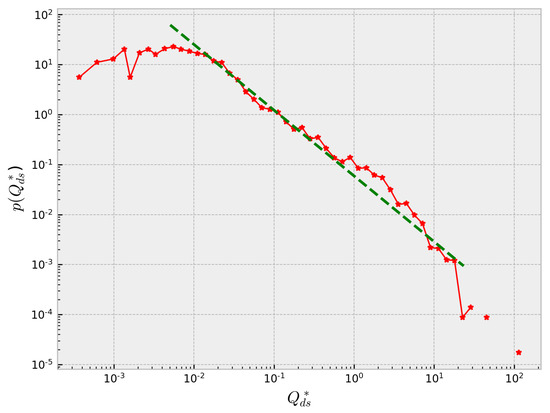
Figure 10.
Plot of the probability density distribution function for normalized . (tons/day) represents the sediment load on days when direct runoff exists. is binned by logarithmic spacing (exponentially increasing width). All the data were normalized by mean daily direct suspended sediment load (tons/day). The cutoff in was set at 0.2. The sediment loads with respect to the direct runoff in the Kabeli River exhibited a power-law model, and the fit is shown by the green dashed line.
In addition, attempts were made to analyze the sediment load with the direct runoff (Figure 11). The comparison of the direct runoff with (the sediment load when exists) made it possible to develop a rating curve. Previously analyzed sediment rating curve methods [5] for the same river have concentrated mostly on filling the incomplete sediment concentration with more complete discharge. These classical rating models are strictly limited to transport-limited systems [10]. In such systems, the sediment concentration is dependent on the available transport capacity, where the sediment is always available and the river is saturated with fine materials. However, an assumption of a transport-limited condition for the incised rivers of the Himalayas would be misleading. As sediment transport is transport-limited on hillslopes, the supply component from the catchments (proxy as ) is predominantly dictating the sediment load in the Kabeli River. This suggests that serves as a better proxy for estimating sediment loads in the Himalayan rivers.
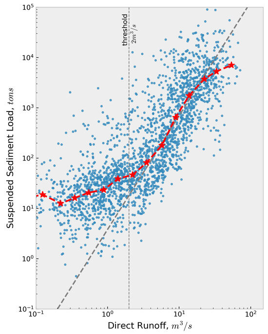
Figure 11.
Bi−logarithmic plot of the suspended sediment load and direct runoff ; binned median of logarithmically equally spaced ranges. The SSL is for days when > 0. The vertical dashed line indicates threshold (2 m3/s), the limit below which the SSL is <1.5% of the yearly load. The inclined dashed line shows a linear relationship.
On a logarithmic scale, the scatter in Figure 11 introduces a bias in log units, as fluctuations toward zero appear larger than fluctuations away from zero. In lower ranges, there are points where the sediment load remains relatively constant. Therefore, a threshold of 2 m3/s is selected by making a qualitative judgment. To account for the small percentage (1.5%) of where is less than this threshold, was added systematically to the modeled . For sediment loads larger than the threshold, smooth curves were fitted to the binned means using least squares regression, weighted by inverse variance, i.e., by the reciprocal of the square of the errors for each binned means. Furthermore, only the data with 90% of the confidence interval for each binned data point were used for analysis. This approach greatly reduces the influence of highly uncertain points in regression [49]. The resulting rating equation is given as .
The underlying notion of this approach is to use direct runoff as a means of estimating the sediment load. The rating curve equation thus obtained was used to estimate the sediment load, which can be compared with the measured one for the 8–year period in Figure 12. As it can be seen in Figure 12, the cumulative sediment load time series fits fairly well excluding some deviation in the recorded sediment load in the years 2012, 2015, and 2018, but the deviation is within the acceptable proximity. In fact, it is difficult to address such sporadic events, which could have resulted from mass wasting, landslide, construction activities, etc. The modeled load from this method was able to capture 84.51% of the total observed load over the study period. The cumulative SSL calculated using the sediment rating relation obtained from the OLS method using the total discharge is shown in Figure 12. The OLS rating curve method could only capture 46% of the total observed load, indicating an SSL underestimation of 54%. The suspended sediment rating curve generated using the direct runoff neither includes bias correction nor the optimization methods to make the observed or estimated load equivalent as it was adopted in Ghimire et al., 2021 [5]. It is based more on the appropriate characterization of the sediment process where is predominantly dictating the sediment load at the outlet in the transport-limited hillslope.
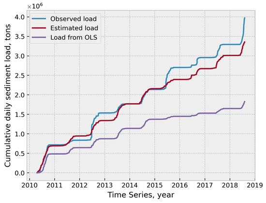
Figure 12.
Observed and estimated cumulative SSL over the study period. The estimated load is calculated using the sediment rating relation obtained from the direct runoff. The load from the OLS is the load calculated from the ordinary least square method.
6. Conclusions
From the analysis, it was found that the suspended sediment in the Kabeli River is interlinked with the distribution of precipitation and more with the direct runoff component of the total discharge. The summer monsoon controls a major portion of sediment yield as approximately 76% of the total annual rainfall occurs during the monsoon season (June–September), resulting in 54% of the total annual flow for the same period, and approximately 90% of the total sediment load gets transported in the same season. Hence, the high seasonal variability in the river flow and sediment load is dominated by the summer monsoon in the Kabeli River and its catchment.
The hysteresis between the river discharge and sediment concentration decreases when the direct runoff is compared with the sediment concentration, which triggered the concept of generating a reproducible relationship. This also suggests that the sediment concentration is influenced by the surface runoff contribution to the total discharge rather than the total stream discharge. The direct runoff could be a better proxy for estimating the sediment concentration than the total stream runoff. This implies that the Kabeli River is supply-limited, and its catchment is transport-limited in terms of sediment yield.
We propose a method for developing sediment rating curves from the direct runoff, which seems promising in this case study. The proposed rating curve model can potentially be used to derive sediment rating curves from observed data in the Himalayan rivers. However, this approach is based only on one river system and should be checked in other rivers with long-term sediment concentration and discharge data before any general recommendation of a rating curve can be made.
In this study, the sediment concentration data are only available without measurements of the bedload. This limitation restricts our analysis to the SSC, potentially overlooking the significant contribution of the bedload to the total sediment load. Future works can focus on the measurement and estimation of the bedload, considering its source-sink relationship and its spatial and temporal dynamics.
Author Contributions
Conceptualization, S.G. and U.S.; methodology formulation, S.G. and U.S.; data investigation, S.G.; analysis, S.G.; resources, U.S., K.K.P. and P.K.B.; writing—original draft preparation, S.G.; writing—reviewing and editing, U.S., K.K.P. and P.K.B.; visualization, S.G.; software, S.G. All authors have read and agreed to published version of this manuscript.
Funding
This research received no external funding.
Data Availability Statement
Data cannot be shared due to confidentiality.
Acknowledgments
The authors are thankful to Kabeli Energy Ltd. for making the sediment and flow data available for this study. The authors are grateful for the timely reply to queries from Christoff Andermann and Yuan Lifeng.
Conflicts of Interest
Author U.S. was employed by the company Hydro Lab Pvt. Ltd., Lalitpur, Nepal. The remaining authors declare that the research was conducted in the absence of any commercial or financial relationships that could be construed as a potential conflict of interest.
Abbreviations
The following abbreviations are used in this manuscript:
| APHRODITE | Asian Precipitation Highly Resolved Observational Data Integration towards Evaluation of Water Resources |
| ASTER | Advanced Spaceborne Thermal Emission and Reflection Radiometer |
| DEM | Digital Elevation Model |
| DHM | Department of Hydrology and Meteorology |
| ICIMOD | International Centre for Integrated Mountain Development |
| ISRIC | International Soil Reference and Information Center |
| KS | Kolmogorov–Smirnov |
| LRMP | Land Resource Mapping Project |
| masl | Meters Above Sea Level |
| MCM | Million Cubic Meters |
| NSE | Nash–Sutcliffe Efficiency |
| OLS | Ordinary Least Square |
| PBIAS | Percentage Bias |
| SOTER | Soils and Terrain Digital Databases |
| SSC | Suspended Sediment Concentration |
| SSL | Suspended Sediment Load |
| SWAT | Soil and Water Assessment Tool |
| Table of Notations | |
| base flow recession parameter | |
| maximum base flow index | |
| Q | total stream runoff |
| base flow | |
| direct runoff | |
| suspended sediment load when > 0 | |
| mean daily direct suspended sediment load | |
| suspended sediment load when > 0, normalized by | |
| R | precipitation |
References
- Milliman, J. River Inputs. In Encyclopedia of Ocean Sciences; Elsevier: Amsterdam, The Netherlands, 2001; pp. 2419–2427. [Google Scholar] [CrossRef]
- Milliman, J.D.; Meade, R.H. World-wide delivery of sediment to the oceans. J. Geol. 1983, 91, 1. [Google Scholar] [CrossRef]
- Roback, K.; Clark, M.K.; West, A.J.; Zekkos, D.; Li, G.; Gallen, S.F.; Chamlagain, D.; Godt, J.W. The size, distribution, and mobility of landslides caused by the 2015 Mw7.8 Gorkha earthquake, Nepal. Geomorphology 2018, 301, 121–138. [Google Scholar] [CrossRef]
- Mahmood, K. Reservoir Sedimentation: Impact, Extent, and Mitigation. World Bank Tech. Pap. Number 1988, 69, 850. [Google Scholar]
- Ghimire, S.; Singh, U.; Bhattarai, P.K. Generation of a Suspended Sediment Rating Curve of a Himalayan River based on a Long-term Data: A case study of Kabeli River. Proc. 10th Ioe Grad. Conf. 2021, 8914, 1110–1118. [Google Scholar]
- Duru, U. Modeling Sediment Yield and Deposition Using the Swat Model. Doctoral Thesis, Colorado State University, Fort Collins, FL, USA, 2015. [Google Scholar]
- Efthimiou, N.; Lykoudi, E.; Karavitis, C. Comparative analysis of sediment yield estimations using different empirical soil erosion models. Hydrol. Sci. J. 2017, 62, 2674–2694. [Google Scholar] [CrossRef]
- Hajigholizadeh, M.; Melesse, A.M.; Fuentes, H.R. Erosion and Sediment Transport Modelling in Shallow Waters: A Review on Approaches, Models and Applications. Int. J. Environ. Res. Public Health 2018, 15, 518. [Google Scholar] [CrossRef] [PubMed]
- Merritt, W.S.; Letcher, R.A.; Jakeman, A.J. A review of erosion and sediment transport models. Environ. Model. Softw. 2003, 18, 761–799. [Google Scholar] [CrossRef]
- Dadson, S.J.; Hovius, N.; Chen, H.; Dade, W.B.; Hsieh, M.L.; Willett, S.D.; Hu, J.C.; Horng, M.J.; Chen, M.C.; Stark, C.P.; et al. Links between erosion, runoff variability and seismicity in the Taiwan orogen. Nature 2003, 426, 648–651. [Google Scholar] [CrossRef] [PubMed]
- Ferguson, R.I. River Loads Underestimated by Rating Curves. Water Resour. Res. 1986, 22, 74–76. [Google Scholar] [CrossRef]
- Duan, N. Smearing estimate: A nonparametric retransformation method. J. Am. Stat. Assoc. 1983, 78, 605–610. [Google Scholar] [CrossRef]
- Annandale, G.; Morris, G.; Karki, P. Extending the Life of Reservoirs: Sustainable Sediment Management for Dams and Run-of-River Hydropower; World Bank Group: Washington, DC, USA, 2016. [Google Scholar]
- Fuller, C.W.; Willett, S.D.; Hovius, N.; Slingerland, R. Erosion rates for Taiwan mountain basins: New determinations from suspended sediment records and a stochastic model of their temporal variation. J. Geol. 2003, 111, 71–87. [Google Scholar] [CrossRef]
- Ponce, V.M. Ultimate Sediment Concentration. In Proceedings of the National Conference on Hydraulic Engineering, Colorado Springs, CO, USA, 8–12 August 1988; pp. 311–315. [Google Scholar]
- Holmes, R.R. Measurement of Bedload Transport in Sand-Bed Rivers: A Look at Two Indirect Sampling Methods. In U.S. Geological Survey Scientific Investigations Report; USGS: Wriston, VA, USA, 2010. [Google Scholar]
- Morin, G.; Lavé, J.; France-Lanord, C.; Rigaudier, T.; Gajurel, A.P.; Sinha, R. Annual Sediment Transport Dynamics in the Narayani Basin, Central Nepal: Assessing the Impacts of Erosion Processes in the Annual Sediment Budget. J. Geophys. Res. Earth Surf. 2018, 123, 2341–2376. [Google Scholar] [CrossRef]
- Lane, E.W.; Borland, W.M. Estimating bed load. Eos, Trans. Am. Geophys. Union 1951, 32, 121–123. [Google Scholar] [CrossRef]
- Pratt-Sitaula, B.; Garde, M.; Burbank, D.W.; Oskin, M.; Heimsath, A.; Gabet, E. Bedload-to-suspended load ratio and rapid bedrock incision from Himalayan landslide-dam lake record. Quat. Res. 2007, 68, 111–120. [Google Scholar] [CrossRef]
- Attal, M.; Lavé, J. Changes of bedload characteristics along the Marsyandi River (central Nepal): Implications for understanding hillslope sediment supply, sediment load evolution along fluvial networks, and denudation in active orogenic belts. In Special Paper of the Geological Society of America Special Papers; Geological Society of America: Boulder, CO, USA, 2006; Volume 398, pp. 143–171. [Google Scholar] [CrossRef]
- Andermann, C.; Crave, A.; Gloaguen, R.; Davy, P.; Bonnet, S. Connecting source and transport: Suspended sediments in the Nepal Himalayas. Earth Planet. Sci. Lett. 2012, 351-352, 158–170. [Google Scholar] [CrossRef]
- Lloyd, C.E.; Freer, J.E.; Johnes, P.J.; Collins, A.L. Using hysteresis analysis of high-resolution water quality monitoring data, including uncertainty, to infer controls on nutrient and sediment transfer in catchments. Sci. Total. Environ. 2016, 543, 388–404. [Google Scholar] [CrossRef] [PubMed]
- Malutta, S.; Kobiyama, M.; Chaffe, P.L.B.; Bonumá, N.B. Hysteresis analysis to quantify and qualify the sediment dynamics: State of the art. Water Sci. Technol. 2020, 81, 2471–2487. [Google Scholar] [CrossRef] [PubMed]
- Asselman, N.E. Suspended sediment dynamics in a large drainage basin: The River Rhine. Hydrol. Process. 1999, 13, 1437–1450. [Google Scholar] [CrossRef]
- Misset, C.; Recking, A.; Legout, C.; Poirel, A.; Cazilhac, M. Geomorphological factors influencing hysteresis patterns between suspended load and flow rate in Alpine rivers. E3s Web Conf. 2018, 40, 1–8. [Google Scholar] [CrossRef]
- Chhetri, A.; Kayastha, R.B.; Shrestha, A. Assessment of Sediment Load of Langtang River in Rasuwa District, Nepal. J. Water Resour. Prot. 2016, 08, 84–92. [Google Scholar] [CrossRef][Green Version]
- Gabet, E.J.; Burbank, D.W.; Pratt-Sitaula, B.; Putkonen, J.; Bookhagen, B. Modern erosion rates in the High Himalayas of Nepal. Earth Planet. Sci. Lett. 2008, 267, 482–494. [Google Scholar] [CrossRef]
- Hasnain, S.I.; Thayyen, R.J. Discharge and suspended-sediment concentration of meltwaters, draining from the Dokriani glacier, Garhwal Himalaya, India. J. Hydrol. 1999, 218, 191–198. [Google Scholar] [CrossRef]
- LRMP. Land Resource Mapping Project: Summary Report; Survey Department, HMGN and Kenting Earth Sciences: Kathmandu, Nepal, 1986. [Google Scholar]
- Andermann, C.; Bonnet, S.; Gloaguen, R. Evaluation of precipitation data sets along the Himalayan front. Geochem. Geophys. Geosystems 2011, 12, 1–16. [Google Scholar] [CrossRef]
- Andermann, C.; Longuevergne, L.; Bonnet, S.; Crave, A.; Davy, P.; Gloaguen, R. Impact of transient groundwater storage on the discharge of Himalayan rivers. Nat. Geosci. 2012, 5, 127–132. [Google Scholar] [CrossRef]
- Ponce, V. Engineering Hydrology: Principles and Practices; Prentice Hall: Saddle River, NY, USA, 1989. [Google Scholar]
- Eckhardt, K. How to construct recursive digital filters for baseflow separation. Hydrol. Process. 2005, 19, 507–515. [Google Scholar] [CrossRef]
- Arnold, J.G.; Allen, P.M. Automated methods for estimating baseflow and ground water recharge from streamflow records. J. Am. Water Resour. Assoc. 1999, 35, 411–424. [Google Scholar] [CrossRef]
- Furey, P.R.; Gupta, V.K. A physically based filter for separating base flow from streamflow time series. Water Resour. Res. 2001, 37, 2709–2722. [Google Scholar] [CrossRef]
- Lim, K.J.; Engel, B.A.; Tang, Z.; Choi, J. Automated Web GIS Based Hydrograph Analysis Tool, WHAT. J. Am. Water Resour. Assoc. 2006, 1397, 1407–1416. [Google Scholar] [CrossRef]
- Wang, Y.; Jiang, R.; Xie, J.; Zhao, Y.; Yan, D.; Yang, S. Soil and Water Assessment Tool (SWAT) Model: A Systemic Review. J. Coast. Res. 2019, 93, 22–30. [Google Scholar] [CrossRef]
- Lee, J.; Kim, J.; Jang, W.; Lim, K.; Engel, B. Assessment of Baseflow Estimates Considering Recession Characteristics in SWAT. Water 2018, 10, 371. [Google Scholar] [CrossRef]
- Moriasi, D.N.; Arnold, J.G.; Liew, M.W.V.; Bingner, R.L.; Harmel, R.D.; Veith, T.L. Model Evaluation Guidelines For Systematic Quantification Of Accuracy In Watershed Simulations. Am. Soc. Agric. Biol. Eng. 2007, 50, 885–900. [Google Scholar] [CrossRef]
- Moriasi, D.N.; Gitau, M.W.; Pai, N.; Daggupati, P. Hydrologic and water quality models: Performance measures and evaluation criteria. Am. Soc. Agric. Biol. Eng. 2015, 58, 1763–1785. [Google Scholar] [CrossRef]
- Tucker, G.E.; Slingerland, R. Drainage basin responses to climate change. Water Resour. Res. 1997, 33, 2031–2047. [Google Scholar] [CrossRef]
- Dahal, R.K.; Hasegawa, S. Representative rainfall thresholds for landslides in the Nepal Himalaya. Geomorphology 2008, 100, 429–443. [Google Scholar] [CrossRef]
- Shrestha, H.S. Sedimentation and Sediment Handling in Himalayan Reservoirs. Doctoral Thesis, Norwegian University of Science and Technology, Trondheim, Norway, 2012. [Google Scholar]
- Alstott, J.; Bullmore, E.; Plenz, D. Powerlaw: A python package for analysis of heavy-tailed distributions. PLoS ONE 2014, 9, 1–18. [Google Scholar] [CrossRef] [PubMed]
- Gillespie, C.S. Fitting heavy tailed distributions: The powerlaw package. J. Stat. Softw. 2015, 64, 1–16. [Google Scholar] [CrossRef]
- Clauset, A.; Shalizi, C.R.; Newman, M.E. Power-law distributions in empirical data. Siam Rev. 2009, 51, 661–703. [Google Scholar] [CrossRef]
- Goldstein, M.L.; Morris, S.A.; Yen, G.G. Problems with fitting to the power-law distribution. Eur. Phys. J. 2004, 41, 255–258. [Google Scholar] [CrossRef]
- Hovius, N.; Stark, C.P.; Hao-Tsu, C.; Jiun-Chuan, L. Supply and removal of sediment in a landslide-dominated mountain belt: Central Range, Taiwan. J. Geol. 2000, 108, 73–89. [Google Scholar] [CrossRef] [PubMed]
- Kirchner, J.W. Catchments as simple dynamical systems: Catchment characterization, rainfall-runoff modeling, and doing hydrology backward. Water Resour. Res. 2009, 45, 1–34. [Google Scholar] [CrossRef]


Disclaimer/Publisher’s Note: The statements, opinions and data contained in all publications are solely those of the individual author(s) and contributor(s) and not of MDPI and/or the editor(s). MDPI and/or the editor(s) disclaim responsibility for any injury to people or property resulting from any ideas, methods, instructions or products referred to in the content. |
© 2024 by the authors. Licensee MDPI, Basel, Switzerland. This article is an open access article distributed under the terms and conditions of the Creative Commons Attribution (CC BY) license (https://creativecommons.org/licenses/by/4.0/).