
Variability of Double-Porosity Flow, Interporosity Flow Coefficient λ and Storage Ratio ω in Dolomites


Department of Geology, Faculty of Natural Sciences and Engineering, University of Ljubljana, Aškerčeva 12, SI-1000 Ljubljana, Slovenia
Water 2024, 16(8), 1072; https://doi.org/10.3390/w16081072
Submission received: 28 February 2024
/
Revised: 1 April 2024
/
Accepted: 6 April 2024
/
Published: 9 April 2024
(This article belongs to the Special Issue Hydraulic and Transient Performances of Pumped-Storage Units)
Abstract
:Seventy-one pumping tests were carried out in various dolomites, revealing two of the less-studied hydrogeological parameters related to double-porosity flow: the interporosity flow coefficient λ and the ratio between storage in the fractures and storage in the whole system (ω). Conceptually, they are both tied to the flow properties of the fractures and matrix and define the communication between these two hydrogeological domains. Five different groups of dolomites were included in this study, with different diagenesis types, crystal sizes, bed thicknesses, fracture intensities and chert contents represented. The results of both parameters reflect variations in the sedimentological and resulting hydrogeological properties of dolomites. The largest values of the interporosity flow coefficient λ (6.53 × 10⁻¹) are found in dolomites formed by late diagenesis, exhibiting the highest degree of fracturing, resulting in fast responses in fractures and large λ values. The values of the storage ratio ω also vary (the range of most values is from 3.32 × 10⁻⁴ to 2.14 × 10⁻¹), with the overall range almost completely filling all the theoretical limits from zero to one. The greatest values of ω are found in dolomites with the largest storage, due to the large number of small fractures, and silica diagenesis probably reduces the matrix storage. The correlations among the parameters show some significant relationships, especially between λ and Km, λ and Sf, ω and Sf, and ω and Sm.
1. Introduction
Analyses of pumping tests in fractured rocks are less common than those in porous aquifers due to their higher complexity and additional parameters. The basic difference is the presence of coupled groundwater flow in the fractures and in the matrix, described and introduced as the double-porosity concept by Barenblatt et al. [1]. For comparison, only one flow regime is analyzed in porous aquifers and only one hydraulic conductivity K and one storage coefficient S are calculated. In double-porosity aquifers, however, each of these two parameters is defined separately for the fractures (Kf, Sf) and for the matrix (Kf, Sf).
Among the less-studied parameters in fractured rocks, two are related to the double-porosity flow: the interporosity flow coefficient (λ) and the ratio between the storage in the fractures and the storage in the whole system (ω), as defined by Warren and Root and later summarized by other authors [2,3,4]. As defined and described later in Section 2.3 and Section 2.4, the interporosity flow coefficient λ indicates how easily water can flow from the matrix blocks of the aquifer into the fractures [2,5], and the omega (ω) is defined as the ratio between the storage in the fractures and the storage in the entire system. They are both conceptually tied to the flow properties in the fractures and the matrix and define the communication between these two hydrogeological domains.
The double-porosity concept was later extended to triple-porosity systems [6,7], where the porosities include the common porosities of the matrix and fractures, as well as the vugs, microfractures and any other cavities occurring in the rock. The original double-porosity model of Warren and Root [2] has been updated by other authors [8], such as Odeh [9], Kazemi [10,11], de Swaan-O [12] and Serra et al. [13], with the introduction of well storage, skin effects [4,14], and other approaches. Reviews of pumping tests in fractured rocks, including data or discussion of the λ and ω, are scarce but have been presented by Gringarten [15] and Kruseman and de Ridder [5].
The motivation for this work lies in the fact that the λ and ω have not been adequately studied for different aquifer lithologies, especially not for dolomites, which exhibit double-porosity properties. The novelty of this approach is to present and discuss the values of both parameters for the different types of dolomites. Some authors have studied both parameters explicitly in the field of oil reservoirs [16] and for two-phase flow (oil + water) [17]. Most studies presented new theoretical models for either pumping test curve behavior or for the determination of either shape factors, interporosity flow coefficients, or new pumping test models, but the range of the studied parameters is rarely given (e.g., in R. Aguilera’s discussion of the Serra et al. paper [13]). It is also interesting that most of the research was carried out in the 1970s and 1980s, and later publications on this topic are quite scarce. Both parameters provide new insights into understanding the behavior of the flow in fractured aquifers and form a basis for further research topics.
2. Materials and Methods
2.1. Dolomites in Slovenia
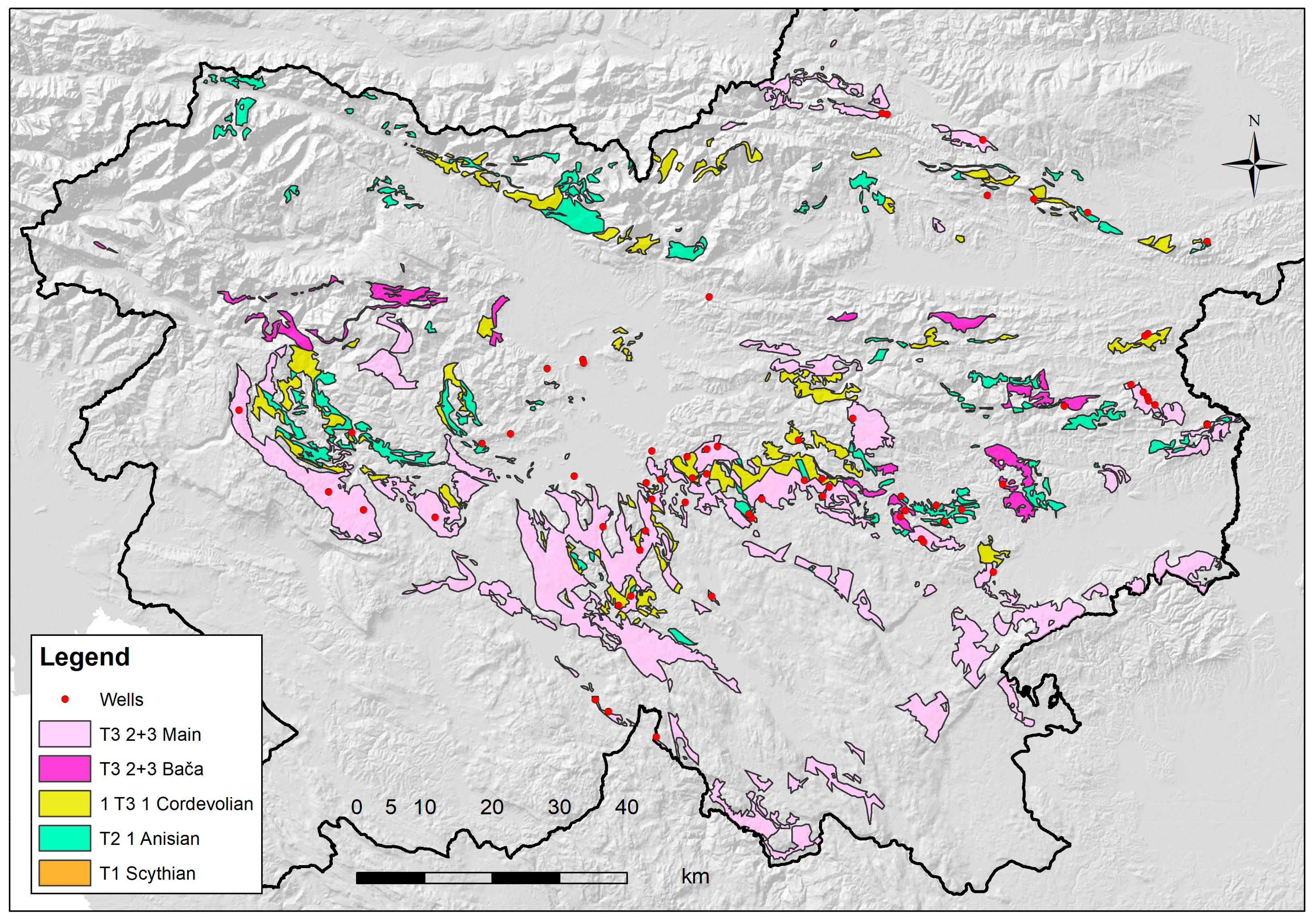
Carbonate rocks are abundant in Slovenia; they outcrop on two-thirds of Slovenia’s ground surface [18,19]. Dolomites outcrop across approximately 8% of the country’s area (Figure 1) and are represented from Permian times, through the Mesozoic and into the earliest parts of the Tertiary. All the dolomites are intensely fractured. Detailed descriptions of all the Slovenian dolomite aquifers (with their sedimentological, hydrogeological and other properties) have been published in several papers [20,21,22,23]. Only those aquifers that are important to this study are discussed here (Table 1). The five groups are, in chronological order: Scythian (T1, Lower Triassic) bedded dolomites with a high clastic component, mostly massive Anisian (T21) pure dolomites, Cordevolian (1T31) late-diagenetic coarse-grained pure dolomites, and two Upper Triassic (T32+3) dolomites: the Bača bedded dolomites with cherts and the bedded Main dolomites with the largest thickness and extent. The latter are also present in neighboring countries under different names. For example, the Main dolomite is found in Italy (where it is known as Dolomia principale) and in Austria (Hauptdolomit). Other dolomites (Permian, Jurassic, Cretaceous, and Tertiary [21]) are presented in Table 1 but are not included in this study because of the scarcity of data and relatively small spatial appearance.
2.2. Pumping Test Data
The dataset was taken from previously performed analyses of the hydraulic conductivities of fractures and matrix in Slovenian dolomites [22]. Seventy-one pumping tests were available for study. Only the wells drilled in dolomites were considered, with a minimum of three wells in the same dolomite group, because statistical analysis was not possible for a group with only one or two wells. All the water wells were drilled for the hydrogeological exploration of groundwater. The wells’ radii (rw) varied from 0.057 to 0.190 m (median value 0.076 m) and the pumping rates varied from 0.25 to 46.00 L/s (median 4.00 L/s).
The hydraulic conductivities and storage coefficients of the fractures and the matrixes were calculated by Barker’s method of the Generalized Radial Flow (GRF) model [24], upgraded to include the double-porosity effects [25]. The calculations were performed by using the AQTESOLV 4.5 software [26]. The output from this method provided the hydraulic conductivity of the fractures and matrix (Kf and Km), the storage coefficients of the fractures and matrix (Sf and Sm), and an additional parameter, called the flow dimension [24] (normally represented by the symbol n, but not to be confused with the number of fractures from Equation (2), the flow dimension here is represented by a subscript nfd), which is related to the fractal geometry of fractures and was analyzed for dolomites in a separate study [23]. The results of the analyses of the Kf, Km, Sf and Sm have already been discussed elsewhere [22] and the main findings of these studies, which are relevant to the discussion of the λ and ω, are discussed here.
For the statistical tests and presentations, Tibco Statistica 13.3 software [27] was used. The Shapiro–Wilk W test was used for testing the statistical distribution, with a significance level α = 5% as a threshold. For the correlations between the studied parameters, the non-parametric Spearman rank order correlation coefficient (r′) was used.
2.3. Interporosity Flow Coefficient (λ)
The interporosity flow coefficient (λ, units [-]) indicates how easily water can flow from the aquifer matrix blocks into the fractures [2,5]. When a fractured aquifer of the double-porosity type is pumped, the interporosity flow coefficient controls the flow in the aquifer.
The interporosity flow coefficient depends on several factors, the most variable and studied of which is the shape factor α [1/m2]:
This shape factor reflects the geometry of the matrix elements and controls the flow between the two porous regions, as originally defined by Warren and Root [2]. It describes the characteristics of the geometry of the fractures and aquifer matrix and depends on the number of normal fracture sets in the rock (n = 1, 2, 3 [-]) and the characteristic length of the matrix blocks (l [m]).
However, the original equation (Equation (2)) is not the only way to calculate the shape factor. Several approaches to the problem have been developed since the publication of the original Warren and Root paper [2]. An extensive comparison of all the approaches was performed by Lim and Aziz [28], Lai and Pao [29] and, finally, Huang et al. [16]. Most methods are based on an analytical or numerical value, multiplied by an inverse value of the equivalent fracture length; this length depends on the number of fracture sets. The shape factor is always reciprocal to the inverse squared value of the fracture length (α ≈ 1/l2).
In this study, the original Warren and Root equation was used. In fact, the interpretation of the λ values in this study does not depend, significantly, on the shape factor used, because the interpretation of the interporosity flow coefficient is based on the relative comparison of different dolomites and will be explained by variations in the hydraulic conductivities, not by the shape factor itself. There are two reasons for such an approach. First, all the models for dolomites consider 3D fractures, which are best approximated by the ‘sugar cube model’, with n = 3 in the Warren–Root model, so there is no variation in the number of fracture sets. Second, the characteristic lengths are very hard to determine due to the highly variable tectonic influence and number, persistence, and density of the fractures. The fault zones in carbonates are spatially highly heterogeneous [30,31,32] and it is hard to define a ‘typical length’. In fact, one can argue that the average distance between the fractures does not exist, as the fractures in dolomites are fractal [23,33,34] and, consequently, they are scale-independent. However, the calculation of the λ values requires a numerical value of characteristic length, so these values were considered to be the same for all the dolomites and fixed at 5 cm, according to personal experience, when performing the extensive hydrogeological studies of all the Slovenian dolomites [21,23,34,35].
Consequently, the shape factor does not change for the studied dolomites and the variability of the interporosity flow coefficient λ is controlled by the two remaining factors in Equation (1); by the ratio between the hydraulic conductivity of the matrix (Km, [m/s or m/day]) and the hydraulic conductivity of the fractures (Kf, [m/s or m/day]), and also the radius of the pumping well rw [m].
Estimation of the interporosity flow coefficient (λ) can also be performed by different approaches. Mostly, the factor is approximated by empirical equations [3,36,37], as reviewed by Rebolledo et al. [38]. In some cases, these authors found the values of λ to be underestimated by up to four orders of magnitude when using Gringarten’s approach [39]. The same authors [38] also stated that ‘Warren and Root offered no solutions for the estimation of λ’. The original equation is, therefore, considered to be difficult to calculate directly and λ is usually calculated by some approximation. In this paper, λ is calculated directly from the original Warren and Root equation (Equation (1)).
2.4. Ratio between Storage in Fractures and Storage in the Whole System (ω)—‘Storage Ratio’
The omega (ω) is defined as the ratio between storage in the fractures and storage in the whole system:
Sf is the storability of the fractures, Sm is the storability of the matrix, and β [-] is a factor for early-time analysis, equal to 0, and for late-time analysis, equal to 1/3 (an orthogonal system, e.g., in dolomites where n = 2, 3) or 1 (where n = 1). Warren and Root [2] also defined ω as a measure of the fluid capacitance of the secondary porosity to that of the combined system. When there is only the primary porosity, Sf equals zero and, consequently, ω = 0 [2].
Alternatively, if the lines of the early and late pumping times are parallel, the omega can also be estimated by different approximations. Authors have used several methods; the horizontal displacement of the two parallel straight lines: ω = t1/t2 [5], from the slope of these two lines: [5], or from the horizontal time ratio of the long-time straight line point to the early time point 1/ω = ΔtDH [4]. However, these two lines should not only be parallel but also straight, and this is rarely the case. Very soon after the publication of the Warren and Root paper, Odeh [9] also disputed the existence of two parallel semi-log straight lines [39], and Gringarten [15] found such parallel straight lines to be very rare (the early-time line can be occluded by storage or skin effects in the well). For these reasons, the original equation (Equation (3)) was used in this contribution.
The workflow is shown below in Figure 2.
3. Results and Discussion
The values of the λ and ω are presented in Table 1, with the geometric mean values, and they are also graphically presented with log-transformed values (Figure 3). The reason to include the geometric mean and the log-transformed values of both parameters is that both the λ and ω are distributed lognormally, as tested by the Shapiro–Wilk W normality test [40] in the Tibco Statistica 13.3 software. For both parameters, the calculated p-value is much below the usual threshold for a statistical significance level of 5% and even below the stricter threshold of 1% (p = 0.0087 for λ and p < 0.0001 for ω), indicating the normal distribution of the log-transformed variables, thus confirming their lognormal distributions. Besides the λ and ω, the geometric means of the hydraulic conductivities (Kf, Km) and storage coefficients (Sf, Sm) of both the fractures and matrixes are presented. These parameters were previously found to be lognormally distributed [19].

Table 1.
Basic statistics for the studied parameters. All the parameters are presented with their geometric means (GMs), except the flow dimension (nfd), which is given as an arithmetic average (this parameter is the only one not lognormally distributed). For the λ and ω, minimum and maximum values are also provided. Units are given in brackets, N = number of samples in each group.
| Dolomite | N | λ-GM [-] | λMIN [-] | λMAX [-] | ω-GM [-] | ω MIN [-] | ω MAX [-] | Kf-GM [m/s] | Km-GM [m/s] | Sf-GM [-] | Sm-GM [-] | nfd [-] |
|---|---|---|---|---|---|---|---|---|---|---|---|---|
| Anisian | 11 | 9.05 × 10⁻² | 1.22 × 10⁻⁵ | 3.57 × 10⁻⁴ | 4.85 × 10⁻⁴ | 9.51 × 10⁻¹² | 1.00 × 100 | 4.13 × 10⁻⁶ | 2.75 × 10⁻⁹ | 1.49 × 10⁻⁵ | 1.63 × 10⁻² | 2.22 |
| Main | 37 | 1.68 × 10⁻¹ | 3.12 × 10⁻⁶ | 7.86 × 10⁻⁸ | 1.10 × 10⁻³ | 5.56 × 10⁻¹³ | 1.00 × 100 | 4.21 × 10⁻⁶ | 4.06 × 10⁻⁹ | 2.18 × 10⁻⁷ | 9.01 × 10⁻⁵ | 2.11 |
| Scythian | 6 | 1.15 × 10⁻¹ | 3.39 × 10⁻⁵ | 7.10 × 10⁻³ | 3.38 × 10⁻³ | 1.02 × 10⁻⁵ | 2.20 × 10⁻¹ | 3.14 × 10⁻⁶ | 2.15 × 10⁻⁹ | 2.13 × 10⁻⁵ | 1.79 × 10⁻² | 1.96 |
| Cordevolian | 14 | 6.53 × 10⁻¹ | 4.07 × 10⁻⁶ | 1.24 × 10⁻⁶ | 4.73 × 10⁻² | 3.42 × 10⁻⁴ | 9.81 × 10⁻¹ | 2.48 × 10⁻⁵ | 9.65 × 10⁻⁸ | 2.04 × 10⁻⁴ | 7.22 × 10⁻³ | 2.34 |
| Bača | 3 | 2.21 × 10⁻² | 3.24 × 10⁻³ | 3.24 × 10⁻¹ | 1.80 × 10⁻³ | 7.64 × 10⁻⁵ | 2.85 × 10⁻² | 2.83 × 10⁻⁵ | 2.83 × 10⁻⁹ | 6.07 × 10⁻⁴ | 1.00 × 100 | 2.19 |
| All Groups | 71 | 1.77 × 10⁻¹ | 3.12 × 10⁻⁶ | 7.86 × 10⁻⁸ | 2.29 × 10⁻³ | 5.56 × 10⁻¹³ | 1.00 × 100 | 6.29 × 10⁻⁶ | 6.66 × 10⁻⁹ | 3.33 × 10⁻⁶ | 1.11 × 10⁻³ | 2.16 |
3.1. Interporosity Flow Coefficient (λ)
The values of λ and ω are presented in Figure 3. It is obvious that the largest values of the interporosity flow coefficient (λ) are found in Cordevolian dolomites (λ = 6.53 × 10⁻¹). There are several reasons for such behavior. These dolomites are significantly more coarse-grained than the others (‘sucrose’ dolomites) and were only formed by late diagenesis [19,20,21,22]. This late diagenesis is one of the processes that can also play a significant role in the aquifer yield, since it tends to increase the grain size, which generally increases the permeability, by up to several orders of magnitude [41,42] through the replacement of interparticle mud with larger crystals from late diagenesis or other processes. As the crystal size increases, the mechanical properties of the dolomites change, making them more brittle than limestone and, therefore, more susceptible to intense fracturing [43,44]. Sucrose and moderately indurated dolomites are most likely to fracture due to their low cohesion strength [45].
Therefore, these dolomites are more susceptible to a higher degree of fracturing [45], leading to a greater number of fractures, including a great number of microfractures, which behave as matrix porosity. Consequently, the interporosity flow from the matrix to the fractures is easiest in Cordevolian dolomites because of their great primary porosity and greater degree of fracturing. Fractures respond very fast to the pumping due to their high frequency and high connectivity (confirmed by the highest n values).
Contrarily, Bača dolomites have the slowest responses, with the lowest geometric mean of λ = 2.21×10⁻², most probably due to the different geological evolution: these dolomites are the only ones with a high proportion of chert, and the diagenetic replacement by silica possibly reduced the porosity (or, more specifically, the intercrystalline porosity, it being responsible for higher permeabilities in dolomites [42]) and hydraulic conductivity of the matrix, leading to lower λ values. One should note the low amount of data for this group (as well as for Scythian dolomites) and the confidence level in Figure 3 is greater than the minimum and maximum values. Other dolomites (Main, Scythian and Anisian) have intermediate values of λ, and they differ by a factor less than 2 (values range from 0.9×10⁻¹ to 1.7×10⁻¹). The hydraulic conductivities of the fractures and matrixes are similar, leading to similar values of λ. For Main and Anisian dolomites, this is somewhat expected, because they are similar in origin (both being very pure dolomites [19,21]). However, Scythian dolomites are much less pure, with much higher clastic contents, and so the Km could be expected to be slightly higher. The results could also be occluded by the small amount of data noted above.
As seen from these results, the values of the interporosity flow coefficient λ do not vary much in general, as the results are quite similar. It is important to note that the λ values would be even greater and more different for Cordevolian dolomites, if the measurements of representative lengths were available, because the distances between the fractures or characteristic length values would be very small compared to other dolomites, leading to greater values of the shape factor and λ values. Influence is important because a small change in length has a big influence on the λ; for example, if the distance between the fractures is reduced from 10 cm to 1 cm (a factor of 10), then the α and λ increase by a factor of 100.
3.2. Ratio between Storage in the Fractures and Storage in the Whole System (ω)
The values of ω show the greatest values in Cordevolian dolomites. These are intensively fractured and, because of the huge number of microfractures, the latter exhibit significant storage capacity. Apart from the numerous fractures, the desiccation pores of Main and Anisian dolomites, despite being mostly filled due to the dolomitization and diagenesis, could also exhibit a small amount of storage, making the total storage in the system (Sf + Sm) larger, leading to smaller values of ω. However, this effect is not so pronounced as to differentiate these dolomites from the others by an order of magnitude or more. Scythian and Bača dolomites are fractured, with no storage in the matrixes, probably due to silica diagenesis or a greater number of fractures, and so the ratio of Sf versus Sf + Sm is larger than those of Main and Anisian dolomites.
The values of ω vary greatly, practically from zero to one (Table 1), filling the complete theoretical range from 0 to 1. However, the range of most values is from 3.32 × 10⁻⁴ to 2.14 × 10⁻¹ (lower and upper quartile values), complying perfectly with the published range from 10−4 to 10−1 in the literature [5,13]. In his reply to Serra et al., Aguilera also presented a review of the ω values (for oil and geothermal reservoirs), spanning from less than 0.006 to 1, thus also filling the complete theoretical range from 0 to 1 [13]. Such a range reflects the range of primary porosity in the rocks; when there is only the primary porosity, there is no storage in the fractures and, consequently, ω = 0 [2].
3.3. Correlations between the Hydrogeological Parameters
The correlations between the hydrogeological parameters show some significant relationships (Table 2). The highest correlation is between the λ and Km, which is somewhat expected from Equation (1); there is a linear dependence of the λ on the hydraulic conductivity of the matrix Km. There is also a negative correlation between the λ and the hydraulic conductivity of the fractures Kf; however, it is not significant. The significance of the correlation between the λ and Sf can be regarded as irrelevant because both parameters are independent, one from the other, and the correlation coefficient is very small (r′ = 0.28). However, there is a significant correlation (r′ = 0.52) between the ω and the storage in the fractures Sf, which also follows on from Equation (3). A negative correlation (r′ = −0.43) exists between the ω and the storage in the matrix Sm, also presumed from the same equation. Similarly significant, but with a medium correlation coefficient, is the correlation between the pumping rate Q and the hydraulic conductivities of the fractures Kf, which is also expected from the pumping tests; water is generally pumped from the fractures and not from the matrix.
4. Conclusions
The values of the interporosity flow coefficient (λ) do not vary as much as the storage ratios (ω), as the results are quite similar. Cordevolian dolomites have the highest values because the fractures respond to pumping very fast due to their great numbers and high connectivity (confirmed by the highest n values). Bača dolomites have the slowest responses and other dolomites have intermediate values. The most probable reason for the similar λ values is that both the hydraulic conductivities of the fractures and the matrixes are very similar, by the same order of magnitude. The λ values would be even greater for Cordevolian dolomites, if the measurements of the characteristic lengths were available, since these values would be very small compared to other dolomites, leading to greater values of the shape factor and λ values. The calculation of λ is very difficult because of the problematic shape factor, which is practically impossible to determine for fractures because they are known to be fractal. In this study, this factor was fixed to some arbitrary value, so the comparison of other factors was possible; in fact, this factor had no influence. The block sizes in dolomites vary greatly and none of the models (slab-shaped or cube-shaped) are truly appropriate, even though the cube-shaped model seems a suitable choice.
The values of the ratio between storage in the fractures and storage in the whole system (ω) show the greatest values in Cordevolian dolomites, which are intensively fractured and, due to the huge number of microfractures, exhibit significant storage capacity. The desiccation pores and fractures in the Main and Anisian dolomites exhibit some noticeable storage, so the total storage in the system (Sf + Sm) is larger, leading to smaller values of the omega. However, this effect is not so pronounced as to differentiate these dolomites from the others by an order of magnitude or more. Scythian and Bača dolomites are purely fractured but with no storage and so the ratio of the Sf versus Sf + Sm is larger than those of Main and Anisian dolomites.
The correlations between the parameters show some significant relationships between the λ, ω and other parameters, especially between the λ and Km (the highest correlation) but also between the λ and Sf, ω and Sf, ω and Sm, and between the pumping rate Q and the hydraulic conductivities of the fractures Kf. All the correlations (except that between the λ and Sf) are rather expected from the theoretical equations.
Further investigations should focus on several topics. First of all, studies should focus on the determination of the shape factor α for each site independently because this would improve the comparison of λ values. Secondly, an investigation into the development of an alternative approach for obtaining the shape factor, suitable for the fractal network of fractures, is necessary because of the problematic determination of α. Thirdly, detailed microscopic analyses of dolomite porosity types and amounts are required because much of the variations in the λ and ω could be explained by this factor. Generally, more data for both parameters in carbonate rocks should be made available in order to perform additional reliable comparisons and interpretations. As presented here, both the λ and ω provide additional insights into understanding the double-porosity flow, which is quite pronounced in carbonates and especially so in dolomites.
Funding
The author acknowledges the Slovenian Research Agency (research core funding No. P1-0195 ‘Geoenvironment and Geomaterials’) for its financial support.
Data Availability Statement
Data are contained within the article.
Acknowledgments
We thank the anonymous reviewers for their constructive comments that improved the quality of the article.
Conflicts of Interest
The author declares no conflicts of interest.
References
- Barenblatt, G.I.; Zheltov, I.P.; Kochina, I.N. Basic concepts in the theory of seepage of homogeneous liquids in fissured rocks. J. Appl. Math. Mech. 1960, 24, 1286–1303. [Google Scholar] [CrossRef]
- Warren, J.E.; Root, P.J. The Behavior of Naturally Fractured Reservoirs. Soc. Pet. Eng. J. 1963, 3, 245–255. [Google Scholar] [CrossRef]
- Bourdet, D.; Gringarten, A. Determination of Fissure Volume and Block Size in Fractured Reservoirs by Type-Curve Analysis. In Proceedings of the SPE Annual Technical Conference and Exhibition, Dallas, TX, USA, 23–25 September 1980. [Google Scholar]
- Mavor, M.J.; Cinco-Ley, H. Transient Pressure Behavior Of Naturally Fractured Reservoirs. In Proceedings of the SPE California Regional Meeting, Ventura, CA, USA, 18–20 April 1979. [Google Scholar]
- Kruseman, G.P.; Ridder, N.A.D. Analysis and Evaluation of Pumping Test Data, 2nd ed.; International Institute for Land Reclamation and Improvement: Wageningen, The Netherlands, 2000; p. 275. [Google Scholar]
- Pulido, H.; Samaniego, V.F.; Rivera, J.; Díaz, F.; Galicia, G. On a Well-Test Pressure Theory of Analysis for Naturally Fractured Reservoirs, Considering Transient Interporosity Matrix, Microfractures, Vugs, and Fractures Flow. In Proceedings of the International Oil Conference and Exhibition in Mexico, Cancun, Mexico, 31 August–2 September 2006. [Google Scholar]
- Liu, J.; Bodvarsson, G.S.; Wu, Y.-S. Analysis of flow behavior in fractured lithophysal reservoirs. J. Contam. Hydrol. 2003, 62–63, 189–211. [Google Scholar] [CrossRef]
- Najurieta, H.L. A Theory for Pressure Transient Analysis in Naturally Fractured Reservoirs. J. Petrol. Technol. 1980, 32, 1241–1250. [Google Scholar] [CrossRef]
- Odeh, A.S. Unsteady-State Behavior of Naturally Fractured Reservoirs. Soc. Pet. Eng. J. 1965, 5, 60–66. [Google Scholar] [CrossRef]
- Kazemi, H. Pressure Transient Analysis of Naturally Fractured Reservoirs with Uniform Fracture Distribution. Soc. Pet. Eng. J. 1969, 9, 451–462. [Google Scholar] [CrossRef]
- Kazemi, H.; Seth, M.S.; Thomas, G.W. The Interpretation of Interference Tests in Naturally Fractured Reservoirs with Uniform Fracture Distribution. Soc. Pet. Eng. J. 1969, 9, 463–472. [Google Scholar] [CrossRef]
- de Swaan, O.A. Analytic Solutions for Determining Naturally Fractured Reservoir Properties by Well Testing. Soc. Pet. Eng. J. 1976, 16, 117–122. [Google Scholar] [CrossRef]
- Serra, K.; Reynolds, A.C.; Raghavan, R. New Pressure Transient Analysis Methods for Naturally Fractured Reservoirs (includes associated papers 12940 and 13014). J. Petrol. Technol. 1983, 35, 2271–2283. [Google Scholar] [CrossRef]
- Moench, A.F. Double-Porosity Models for a Fissured Groundwater Reservoir with Fracture Skin. Water Resour. Res. 1984, 20, 831–846. [Google Scholar] [CrossRef]
- Gringarten, A.C. Flow-Test Evaluation of Fractured Reservoirs. In Recent Trends in Hydrogeology; Geological Society of America Special Papers; Geological Society of America: Boulder, CO, USA, 1982; pp. 237–264. [Google Scholar]
- Huang, S.; Ma, X.; Yong, R.; Wu, J.; Zhang, J.; Wu, T. Transient Interporosity Flow in Shale/Tight Oil Reservoirs: Model and Application. ACS Omega 2022, 7, 14746–14755. [Google Scholar] [CrossRef]
- Al-Bemani, A.S.; Ershaghi, I. Two-Phase Flow Interporosity Effects on Pressure Transient Test Response in Naturally Fractured Reservoirs. In Proceedings of the SPE Annual Technical Conference and Exhibition, Dallas, TX, USA, 6–9 October 1991. [Google Scholar]
- Ogorelec, B.; Dolenec, T.; Pezdič, J. Isotope composition of O and C in Mesosoic carbonate rocks of Slovenia—Effect of facies and diagenesis. Geologija 1999, 42, 171–205. [Google Scholar] [CrossRef]
- Verbovšek, T.; Veselič, M. Factors influencing the hydraulic properties of wells in dolomite aquifers of Slovenia. Hydrogeol. J. 2008, 16, 779–795. [Google Scholar] [CrossRef]
- Verbovšek, T. Estimation of transmissivity and hydraulic conductivity from specific capacity and specific capacity index in dolomite aquifers. J. Hydrol. Eng. 2008, 13, 817–823. [Google Scholar] [CrossRef]
- Verbovšek, T. Diagenetic effects on the well yield of dolomite aquifers in Slovenia. Environ. Geol. 2008, 53, 1173–1182. [Google Scholar] [CrossRef]
- Verbovšek, T. Hydraulic conductivities of fractures and matrix in Slovenian carbonate aquifers. Geologija 2008, 51, 245–255. [Google Scholar] [CrossRef]
- Verbovšek, T. Influences of Aquifer Properties on Flow Dimensions in Dolomites. Ground Water 2009, 47, 660–668. [Google Scholar] [CrossRef]
- Barker, J.A. A Generalized Radial Flow Model for Hydraulic Tests in Fractured Rock. Water Resour. Res. 1988, 24, 1796–1804. [Google Scholar] [CrossRef]
- Hamm, S.-Y.; Bidaux, P. Dual-Porosity Fractal Models for Transient Flow Analysis in Fissured Rocks. Water Resour. Res. 1996, 32, 2733. [Google Scholar] [CrossRef]
- Hydrosolve. AQTESOLV for Windows; Version 4.5; Hydrosolve Inc.: Reston, VA, USA, 2006. [Google Scholar]
- StatSoft GmbH. Tibco Statistica; Version 13.3; StatSoft GmbH: Hamburg, Germany, 2019. [Google Scholar]
- Lim, K.T.; Aziz, K. Matrix-fracture transfer shape factors for dual-porosity simulators. J. Petrol. Sci. Eng. 1995, 13, 169–178. [Google Scholar] [CrossRef]
- Lai, K.S.; Pao, W.K.S. Assessment of Different Matrix-fracture Shape Factor in Double Porosity Medium. J. Appl. Sci. 2013, 13, 308–314. [Google Scholar] [CrossRef]
- Bauer, H.; Schröckenfuchs, T.C.; Decker, K. Hydrogeological properties of fault zones in a karstified carbonate aquifer (Northern Calcareous Alps, Austria). Hydrogeol. J. 2016, 24, 1147–1170. [Google Scholar] [CrossRef]
- Čar, J. Geostructural mapping of karstified limestones. Geologija 2018, 61, 133–162. [Google Scholar] [CrossRef]
- Caine, J.S.; Evans, J.P.; Forster, C.B. Fault zone architecture and permeability structure. Geology 1996, 24, 1025–1028. [Google Scholar] [CrossRef]
- Pavičić, I.; Duić, Ž.; Vrbaški, A.; Dragičević, I. Fractal Characterization of Multiscale Fracture Network Distribution in Dolomites: Outcrop Analogue of Subsurface Reservoirs. Fractal Fract. 2023, 7, 676. [Google Scholar] [CrossRef]
- Verbovšek, T. Extrapolation of fractal dimensions of natural fracture networks from one to two dimensions in dolomites of Slovenia. Geosci. J. 2009, 13, 343–351. [Google Scholar] [CrossRef]
- Verbovšek, T.; Kanduč, T. Isotope Geochemistry of Groundwater from Fractured Dolomite Aquifers in Central Slovenia. Aquat. Geochem. 2015, 22, 131–151. [Google Scholar] [CrossRef]
- Uldrich, D.O.; Ershaghi, I. A Method for Estimating the Interporosity Flow Parameter in Naturally Fractured Reservoirs. Soc. Pet. Eng. J. 1979, 19, 324–332. [Google Scholar] [CrossRef]
- Crawford, G.E.; Hagedorn, A.R.; Pierce, A.E. Analysis of Pressure Buildup Tests in a Naturally Fractured Reservoir. J. Petrol. Technol. 1976, 28, 1295–1300. [Google Scholar] [CrossRef]
- Rebolledo, L.C.; Ershaghi, I. Errors in Estimating Interporosity Flow Coefficient in Naturally Fractured Reservoirs. In Proceedings of the SPE Annual Technical Conference and Exhibition, Houston, TX, USA, 28–30 September 2015. [Google Scholar]
- Gringarten, A.C. Interpretation of Tests in Fissured and Multilayered Reservoirs With Double-Porosity Behavior: Theory and Practice. J. Petrol. Technol. 1984, 36, 549–564. [Google Scholar] [CrossRef]
- de Sá, M.; Joaquim, P. Applied Statistics Using SPSS, STATISTICA, MATLAB and R.; Springer: Berlin, Germany, 2007; p. 505. [Google Scholar]
- Negra, M.H.; Purser, B.H.; M’Rabet, A. Permeability and Porosity Evolution in Dolomitized Upper Cretaceous Pelagic Limestones of Central Tunisia. In Dolomites; Blackwell Publishing Ltd.: London, UK, 2009; pp. 309–323. [Google Scholar]
- Warren, J. Dolomite: Occurrence, evolution and economically important associations. Earth-Sci. Rev. 2000, 52, 1–81. [Google Scholar] [CrossRef]
- Stearns, D.W.; Friedman, N. Reservoirs in Fractured Rock. In AAPG Memoir 16: Stratigraphic Oil and Gas Fields—Classification, Exploration Methods, and Case Histories; Gould, H.R., Ed.; American Association of Petroleum Geologists (AAPG): Tulsa, OK, USA, 1972; Volume 16, pp. 82–106. [Google Scholar]
- Aguilera, R. Naturally Fractured Reservoirs; PennWell Books: Tulsa, OK, USA, 1980. [Google Scholar]
- Gaswirth, S.B.; Budd, D.A.; Crawford, B.R. Textural and stratigraphic controls on fractured dolomite in a carbonate aquifer system, Ocala limestone, west-central Florida. Sediment. Geol. 2006, 184, 241–254. [Google Scholar] [CrossRef]
Figure 1.
Map of the studied dolomites in Slovenia and locations of the studied wells.

Figure 2.
Complete workflow for the investigated parameters. Steps 2 to 4 were performed prior to this study in the investigation of the hydraulic conductivities of the fractures and matrixes in Slovenian dolomites [22]. The fieldwork in step 3 was carried out on the basis of the field photographs, where these were available.
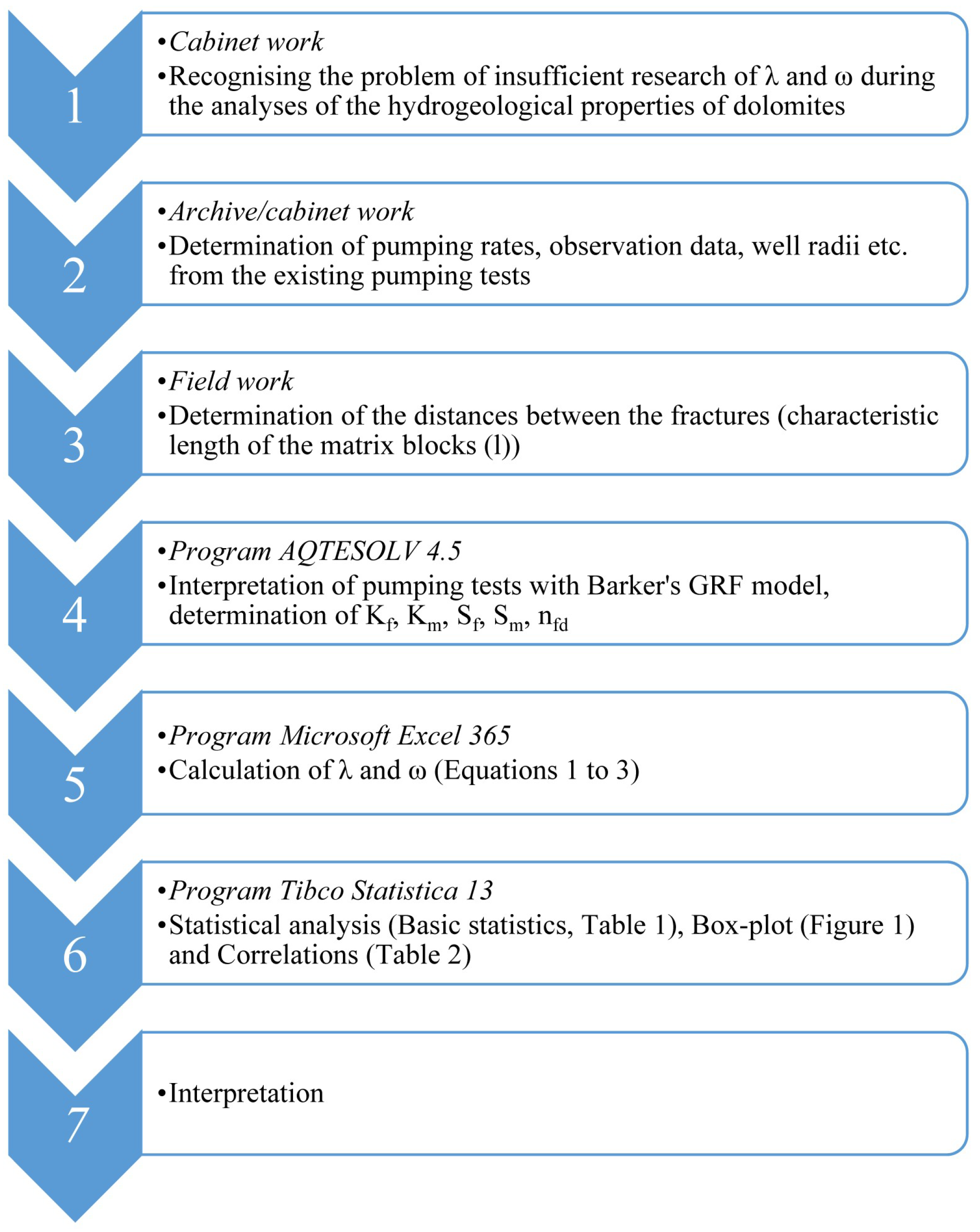
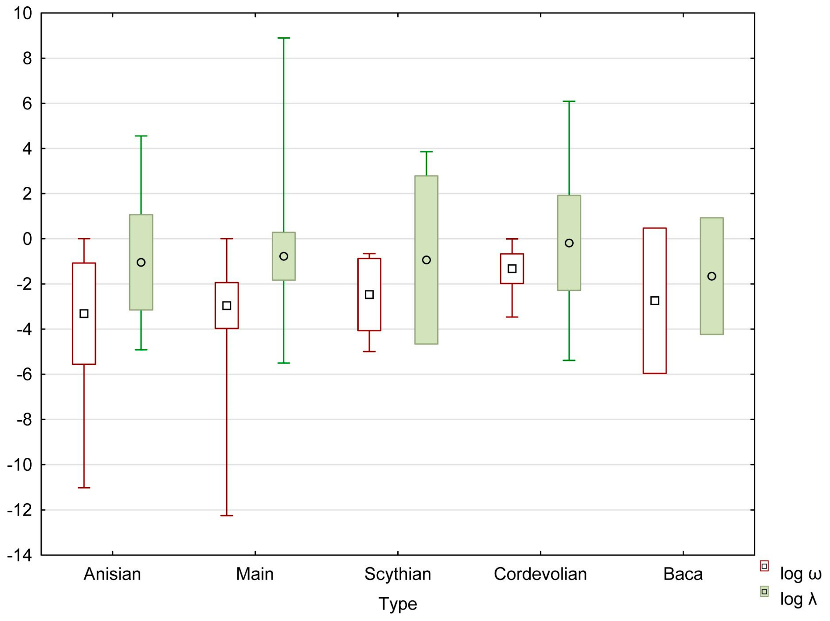
Figure 3.
Log-transformed values of λ and ω (both dimensionless). Small squares and circles indicate the geometric means; box limits define the 0.95 confidence interval and whiskers indicate the minimum and maximum values.
Figure 3.
Log-transformed values of λ and ω (both dimensionless). Small squares and circles indicate the geometric means; box limits define the 0.95 confidence interval and whiskers indicate the minimum and maximum values.

Table 2.
Spearman rank order correlation coefficients (r′). Correlations marked with an asterisk (*) are significant at 5% significance level.
Table 2.
Spearman rank order correlation coefficients (r′). Correlations marked with an asterisk (*) are significant at 5% significance level.
| Duration [min] | Q [L/s] | Kf [m/s] | Sf [-] | Km [m/s] | Sm [-] | rw [m] | ω [-] | λ [-] | |
|---|---|---|---|---|---|---|---|---|---|
| Duration [min] | 1.000 | 0.070 | 0.179 | 0.174 | −0.025 | 0.081 | −0.026 | 0.130 | −0.093 |
| Q [L/s] | 0.070 | 1.000 | 0.563 * | 0.058 | 0.149 | −0.080 | 0.022 | 0.060 | 0.004 |
| Kf [m/s] | 0.179 | 0.563 * | 1.000 | 0.132 | 0.087 | −0.060 | −0.058 | 0.157 | −0.209 |
| Sf [-] | 0.174 | 0.058 | 0.132 | 1.000 | 0.341 * | 0.418 * | −0.190 | 0.521 * | 0.284 * |
| Km [m/s] | −0.025 | 0.149 | 0.087 | 0.341 * | 1.000 | 0.084 | 0.033 | 0.227 | 0.940 * |
| Sm [-] | 0.081 | −0.080 | −0.060 | 0.418 * | 0.084 | 1.000 | −0.028 | −0.430 * | 0.096 |
| rw [m] | −0.026 | 0.022 | −0.058 | −0.190 | 0.033 | −0.028 | 1.000 | −0.136 | 0.064 |
| ω [-] | 0.130 | 0.060 | 0.157 | 0.521 * | 0.227 | −0.430 * | −0.136 | 1.000 | 0.179 |
| λ [-] | −0.093 | 0.004 | −0.209 | 0.284 * | 0.940 * | 0.096 | 0.064 | 0.179 | 1.000 |
Disclaimer/Publisher’s Note: The statements, opinions and data contained in all publications are solely those of the individual author(s) and contributor(s) and not of MDPI and/or the editor(s). MDPI and/or the editor(s) disclaim responsibility for any injury to people or property resulting from any ideas, methods, instructions or products referred to in the content. |
© 2024 by the author. Licensee MDPI, Basel, Switzerland. This article is an open access article distributed under the terms and conditions of the Creative Commons Attribution (CC BY) license (https://creativecommons.org/licenses/by/4.0/).
Share and Cite
MDPI and ACS Style
Verbovšek, T. Variability of Double-Porosity Flow, Interporosity Flow Coefficient λ and Storage Ratio ω in Dolomites. Water 2024, 16, 1072. https://doi.org/10.3390/w16081072
AMA Style
Verbovšek T. Variability of Double-Porosity Flow, Interporosity Flow Coefficient λ and Storage Ratio ω in Dolomites. Water. 2024; 16(8):1072. https://doi.org/10.3390/w16081072
Chicago/Turabian StyleVerbovšek, Timotej. 2024. "Variability of Double-Porosity Flow, Interporosity Flow Coefficient λ and Storage Ratio ω in Dolomites" Water 16, no. 8: 1072. https://doi.org/10.3390/w16081072
Note that from the first issue of 2016, this journal uses article numbers instead of page numbers. See further details here.