The Hourly Peak Coefficient of Single-Family and Multi-Family Buildings in Poland: Support for the Selection of Water Meters and the Construction of a Water Distribution System Model

Abstract

Taking care of water resources and minimizing water losses in water supply networks requires a broad approach to identifying and neutralizing operational problems. The correct selection of water meters to minimize apparent losses requires knowledge of the characteristic flows that may occur in the facility to which water is supplied. The research aimed to develop tools in the form of mathematical models and water consumption curves along with hourly water consumption coefficients to facilitate the process of selecting water meters for engineers and creating computer models of water supply systems. The research involved monitoring the flow of 76 single-family and multi-family buildings in four towns in Poland, followed by data analysis and development of tools supporting the selection of water meters and the construction of computer models of water distribution networks. High correlation coefficients of the studied variables indicate the results’ usefulness. Four models were developed to determine the maximum flow values in multi-family buildings (three models) and single-family buildings (one model) in the range of water meter diameters DN15-DN40. Characteristics of the average hourly peak coefficient (HPC) values were also developed, along with the range of changes in HPC values for single-family and multi-family buildings.

1. Introduction

A water distribution system (WDS), as a set of facilities and devices ensuring the supply of water with appropriate qualitative and quantitative parameters for domestic, industrial and fire-fighting needs, is critical infrastructure for the proper and sustainable functioning of modern society [1]. Therefore, the optimal design, operation, and management of WDSs are the subject of numerous studies and analyses. Among them, optimal system management is of particular importance, including partitioning into district-metered areas (DMA) [2,3], the location of pressure-reducing valves (PRVs) [4], or the use of integrated tools connecting capital, operations, and supporting systems (workforce, customers, and stakeholders) [5].

The main component of a WDS is the water distribution network (WDN), consisting of water pipes that supply water to consumers. Each WDN is characterized by variability in terms of water supplies during the day. Most often, there are periods of increased (peak) water consumption during the day, e.g., the morning peak and evening peak, periods of minimal water consumption at night or even no water consumption at night and periods of average water consumption from morning to evening during the day [6]. The variability of water consumption applies not only to the day but also to individual days of the week or months. Water consumption depends on the number of inhabitants, the condition of the water distribution network, the type of settlement unit (town or village), and character (industrial agglomeration, service area, or tourist areas) [7]. The variability of water consumption affects many operational aspects:

• The selection of pipe diameter for a water distribution network (WDN) [8,9];
• The selection of water meter size for consumers [10];
• Control characteristics and number of pump units [11,12,13];
• The necessity to build field reservoirs [14].

For each hour of the day, we can determine the value of the hourly peak coefficient (HPC), also known as the non-uniformity index of water consumption [15].

Research conducted by the research office in Italy has shown that as the number of inhabitants of a settlement unit increases, HPC values decrease, and the range of obtained values narrows. For example, for towns with fewer than 500 inhabitants, the HPC value varies from 3.00 to 5.00, and for towns with more than 50,000 inhabitants, HPC values range from 2.00 to 2.50. The data were taken from 129 towns located in the Puglia region (Southern Italy) from 2008 to 2010. The data were recorded for about seven days in 3, 5, or 10 min intervals. Almost 85% of the population ranges between 1900 and 40,000 inhabitants. These studies demonstrated the validity of using water consumption measurement intervals from several seconds to several minutes and showed that as the number of inhabitants in the city decreases, the HPC increases [16].

Research conducted in Poland showed changes in the maximum HPC values from approximately 1.3 to 1.8 [17,18,19]. The study conducted in Poland, similar to the study from Italy, showed the validity of using water consumption measurement intervals from several seconds to several minutes and showed that as the number of inhabitants in a city decreases, the HPC increases.

Research carried out by Gwoździej-Mazur and Świętochowski for two rural water distribution networks in the Podlaskie Voivodeship in Poland allowed for the obtainment of daily curves for entire systems with HPC values from 0.00 to 2.00 during the period of maximum water consumption during the day. The average daily flow changes throughout the year from 0.65 for months with minimum water consumption in the settlement unit to 1.83, which was observed during the period of maximum water consumption by the residents [15].

Research conducted in Chihuahua City, Mexico, showed HPC changes from 0.07 to 1.64 [20]. Research conducted in Cracow, Poland, showed a maximum post-winter HPC of 1.77 [21].

It is worth noting that in most studies based on the analysis of measurements of actual water consumption in WDN, the obtained HPC values are lower than those given by the national or local design standards, which can be explained by the increasingly widespread water saving solutions used in sanitary fittings [22]. In most countries, the normative HPC value depends on the population (p) served by the water supply network, and mathematical models are based on an inverse power–law relationship applied to the p-value. For example, based on the German design guideline of DVGW-w410, HPC values should range from 5.5 for systems with p < 5000 to 2.2 for systems with p = 500,000–1,000,000. In turn, the guidelines of the Ministry of Environment of the Canadian province of Ontario, based on empirical relationships, provide values ranging from 4.30 for p = 500 to 3.00 for p = 3001–10,000 (exemplary values) [23]. In Poland, HPC values recommended in the past (but not currently in force) range from 3.5 for single-family buildings with incomplete sanitary facilities, through 2.5 for multi-family buildings and p = 10,000, to 1.8 for multi-family buildings and towns with p > 500,000 inhabitants [24].

The development of consumption curves and the values of maximum flows in a settlement unit is important and necessary during the construction of hydraulic models, which are used to develop network operation scenarios as well as for modernization and operation optimization [25]. An important process of building models is calibration based on recorded flow and pressure values. Measurement campaigns (field research) are time-consuming and require high costs. Sharing already developed values allows engineers to deliver useful computer models faster.

When caring for natural resources, especially drinking water resources, it is necessary to provide water sustainably. This involves, among other things, supplying water to consumers through a water distribution network with the lowest possible level of water losses. Water losses may occur as real losses—water leaks from the network into the ground or as apparent losses, i.e., related to the method of measuring water sold to customers [26]. Among the methods of minimizing apparent losses, there are issues with the selection of water meters and their measurement accuracy [10,27].

Selecting the correct size of water meters requires knowledge of the average expected water consumption during the day and the values of maximum and minimum flows that may occur in each facility. The maximum values are important so that the size of the water meter and its water flow capacity can ensure an uninterrupted water supply at maximum water consumption. On the other hand, the value of the minimum flow that the water meter can register must be lower than the expected minimum water consumption in the facility. Otherwise, the facility may consume water, but the consumption value will not be recorded, and thus, apparent losses will occur. The largest possible volume of water consumed by consumers in the building must be between q2 water meter and q3 (nominal value—definition from Directive 2014/32/EU [28]), where the accuracy of water meters is the highest, and thus, the apparent losses are minimized.

It is therefore justified to conduct research aimed at providing tools for engineers dealing with water meter management and the operation of the water distribution system in the form of mathematical models that facilitate the determination of maximum water flows in buildings and the determination of water consumption curves along with HPC coefficients to facilitate the design of hydraulic models and their subsequent calibration without performing costly measurement campaigns.

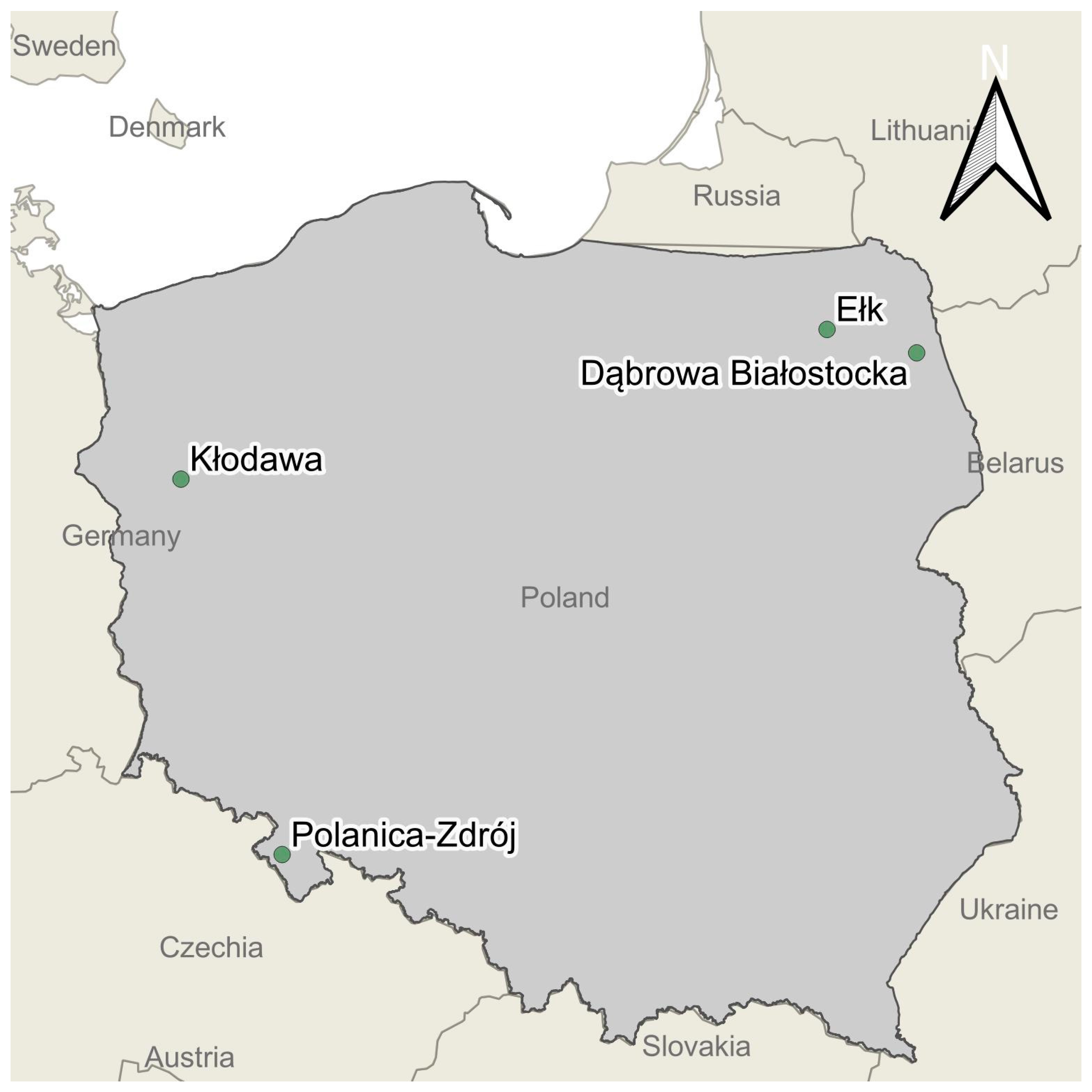
2. Materials and Methods

Field research was conducted on selected single-family and multi-family buildings in 4 towns in different parts of Poland (Figure 1). A single-family building is a detached building or a semi-detached, terraced or group building used to meet housing needs, constituting a structurally independent whole in which no more than two residential premises may be separated [29]. A building with a separate number of residential units greater than two units intended for collective accommodation is called a multi-family building. The towns had a population of 5300–6800 inhabitants. The towns belong to a group of urban areas with a tourist character. The research was conducted at different times of the year, both during periods of low water consumption and during the tourist season. Water meters in Poland are installed once every 5 years, and their size should be selected to ensure correct operation throughout the entire period of use of the water meter. The buildings included in the research are supplied with a continuous water supply system.

The buildings are supplied by municipal WDNs. House connections are equipped with water meters with various accuracy classes for measuring water volume. The research was carried out using measurement sets (Figure 2) consisting of water meters with metrological class R ≥ 160 for diameters from DN15 to DN40 and data recorders mounted directly to the water meter counter. The measurement resolution was set at an interval of every 15 min. Measurements were carried out continuously—24 h a day. The duration of observation of one object was a minimum of 14 days. The measurement interval was selected based on the author’s previous experience [15,30] and other literature data [16,31,32], as well as consideration of the measurement range of the data recorders and the resolution of the water meters—DN15-DN32 is 0.001 dm³ and DN40 is 0.01 dm³. Choosing too short an interval for recording data from the water meter leads to too many distorted measurements, and too long an interval period leads to a shallower daily consumption curve and a loss of the recorded maximum flow values in their actual value.

A total of 76 single-family buildings (DN15 and DN20 water meters—Figure 2(3)) and multi-family buildings (DN20-DN40—Figure 2(4) were tested. Technical characteristic of flow meters used in this research is presented in

Table 1. The table shows the ranges of flow meters used in the field study for single-family buildings and multi-family buildings.

DN [mm]	Qstart [m3/h]	Q1 [m3/h]	Q2 [m3/h]	Q3 [m3/h]	Q4 [m3/h]
Single-Family Bulidings
15	0.003	0.0156	0.250	2.500	3.100
20	0.005	0.0250	0.040	4.000	5.000
Multi-Family Bulidings
20	0.005	0.0250	0.040	4.000	5.000
25	0.010	0.0394	0.063	6.300	7.800
32	0.012	0.0625	0.100	10.000	12.500
40	0.013	0.1000	0.160	16.000	20.000

.

The analyses were carried out using the relationship between the average hourly flow and daily consumption and between the average maximum hourly flow and daily consumption. The median values of diameter and maximum flows were also taken into account.

When determining the peak hourly values, which were available in the literature, a general formula for the non-uniformity index was used [33]:

$$N_{t,a}=\frac{Q_{t,a}}{Q_{tavg}}$$

(1)

where: N_t,a is non-uniformity index, Q_t,a is volume of water pumped into the WDN over time t, [m³/t], Q_{t avg} is mean volume of water pumped into WDN over time t, [m³/t], t is unit of time, [month, day, hour] and a is discriminant of the maximum or minimum index for a given unit of time t.

Data collected in the field measurement campaign required some preliminary selection. Additionally, towns with significant touristic fluctuation and data characterized by abnormal water supply, probably due to special regulations carried out by the managing authority or affected by instrumental measuring errors, were excluded from the first analyses.

3. Results and Discussion

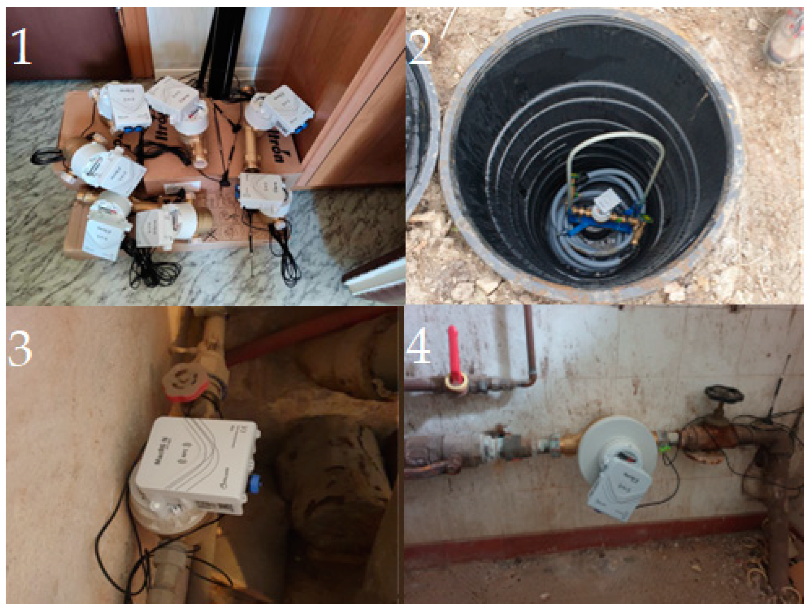
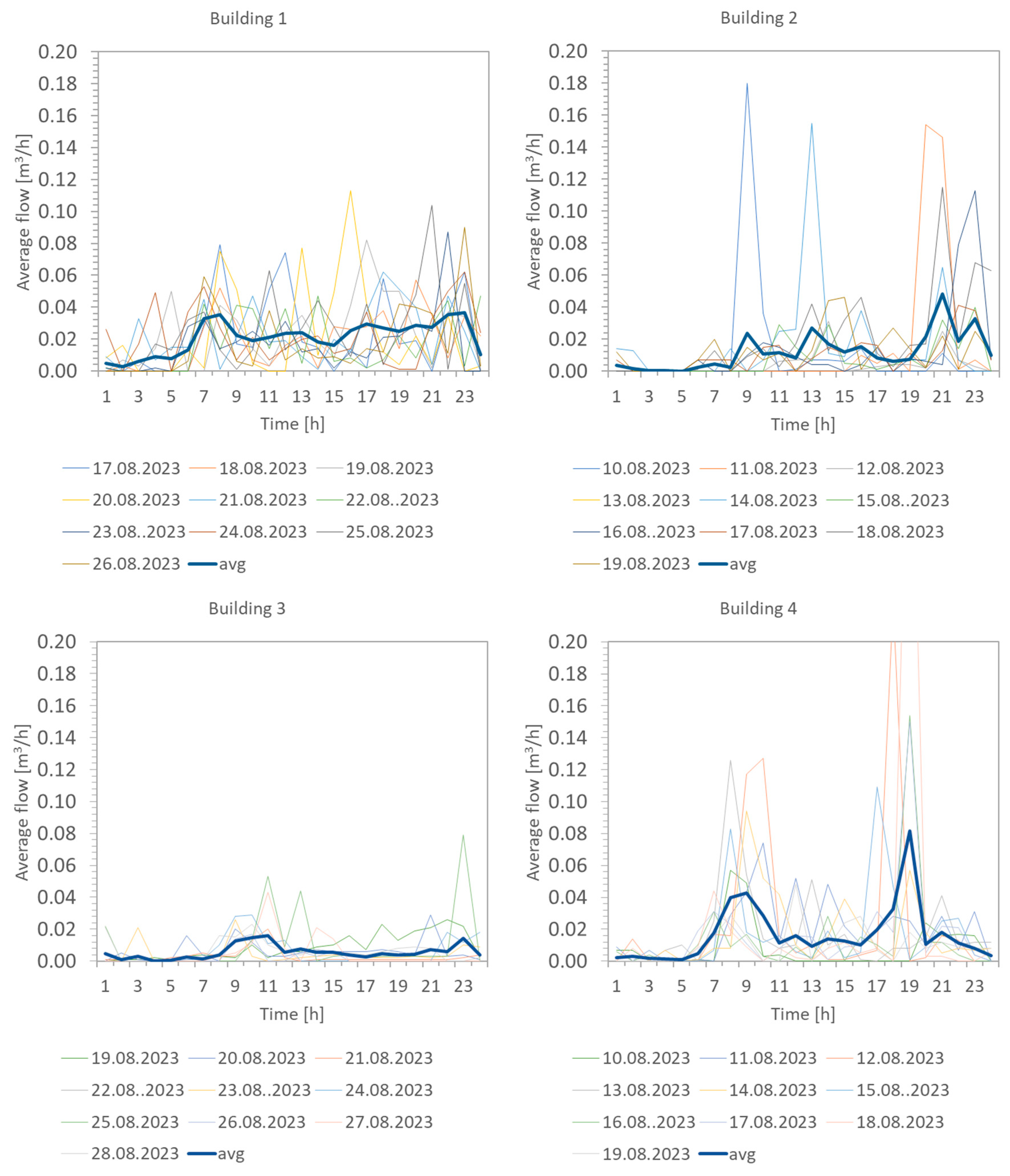
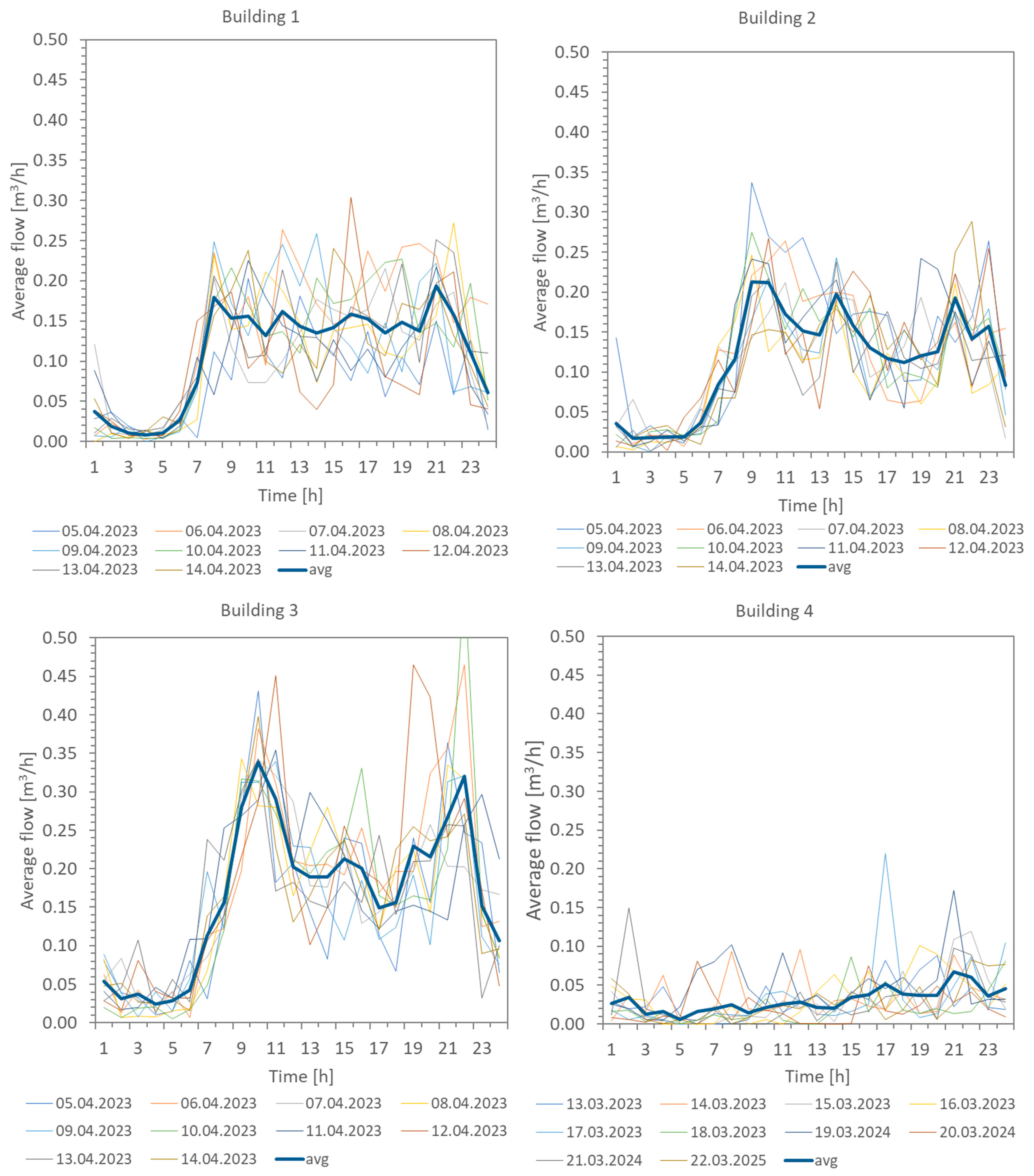
3.1. Results of Water Meter Monitoring

During field measurements, the following parameters were obtained:

• Daily consumption values;
• Flow values for the interval time = 15 min;
• Maximum and minimum flow values during the day;
• Maximum and minimum flow values in each hour.

Figure 3 shows graphs of recorded flow values for four selected single-family buildings during the day. The charts present 10 daily curves and a curve of the average hourly flow value for each hour. The curves presented reflect four types of water consumption in single-family buildings. Building 1 shows a daily consumption curve typical of single-family buildings where water is collected 24 h a day. This may be due to professional nature or lifestyle and household responsibilities. There is no visible regularity or repetition of residents’ behavior throughout the day or week. Building 2 shows a daily consumption curve typical of single-family buildings, whose inhabitants have a regular lifestyle during the day and week, with a visible peak in water consumption in the morning and evening, as well as increased water consumption during the lunch period. Building 3 shows a characteristic curve for a group of single-family buildings inhabited by single persons or elderly people with low water consumption needs. A very low flow is observed here, with an average value less than 0.020 m³/h. Building 4 shows a water consumption curve typical of literature data, which shows two increased water consumption periods: morning and evening peaks, as well as low or zero flow at night and average flows during the day.

Figure 4 shows graphs of recorded flow values for four selected multi-family buildings, whose consumption curves correspond to the characteristic types of water consumption observed during field measurements. Building 1 represents a group of multi-family buildings in which residents use water almost evenly around the clock. Water consumption curves during the day show characteristic increased water consumption in the morning, noon, and evening, but this consumption is not regular and repeatable every day. The averaged flow curve is characterized by increased and almost uniform water consumption from 7 a.m. to 10 p.m. Building 2 represents a group of multi-family buildings with water consumption during the day typical of multi-family buildings [34]. There are three periods of increased water consumption: morning, afternoon, and evening. The repeatability of both the consumption curves for single days and the average values over the measurement period is visible. It is also characteristic that the highest water consumption during the day is in the morning, around 8 a.m. However, the peak water consumption at lunch and in the evening is lower than in the morning. High water consumption during lunchtime will reduce the needs of residents in the evening. Building 3 represents a group of multi-family buildings with the most characteristic daily distribution curve. The two largest water consumptions are visible: in the morning and the evening. Additionally, increased water consumption is visible during lunch, but its value is much lower than water use in the morning and evening. Building 4 shows daily water consumption curves for a characteristic group of buildings in which internal installations are in poor technical condition (age of installations, quality of materials, failures of sanitary fittings). A flattening of the daily water consumption curve is visible, with individual periods of increased water consumption. These buildings are characterised by low water consumption by residents and high levels of water leakage.

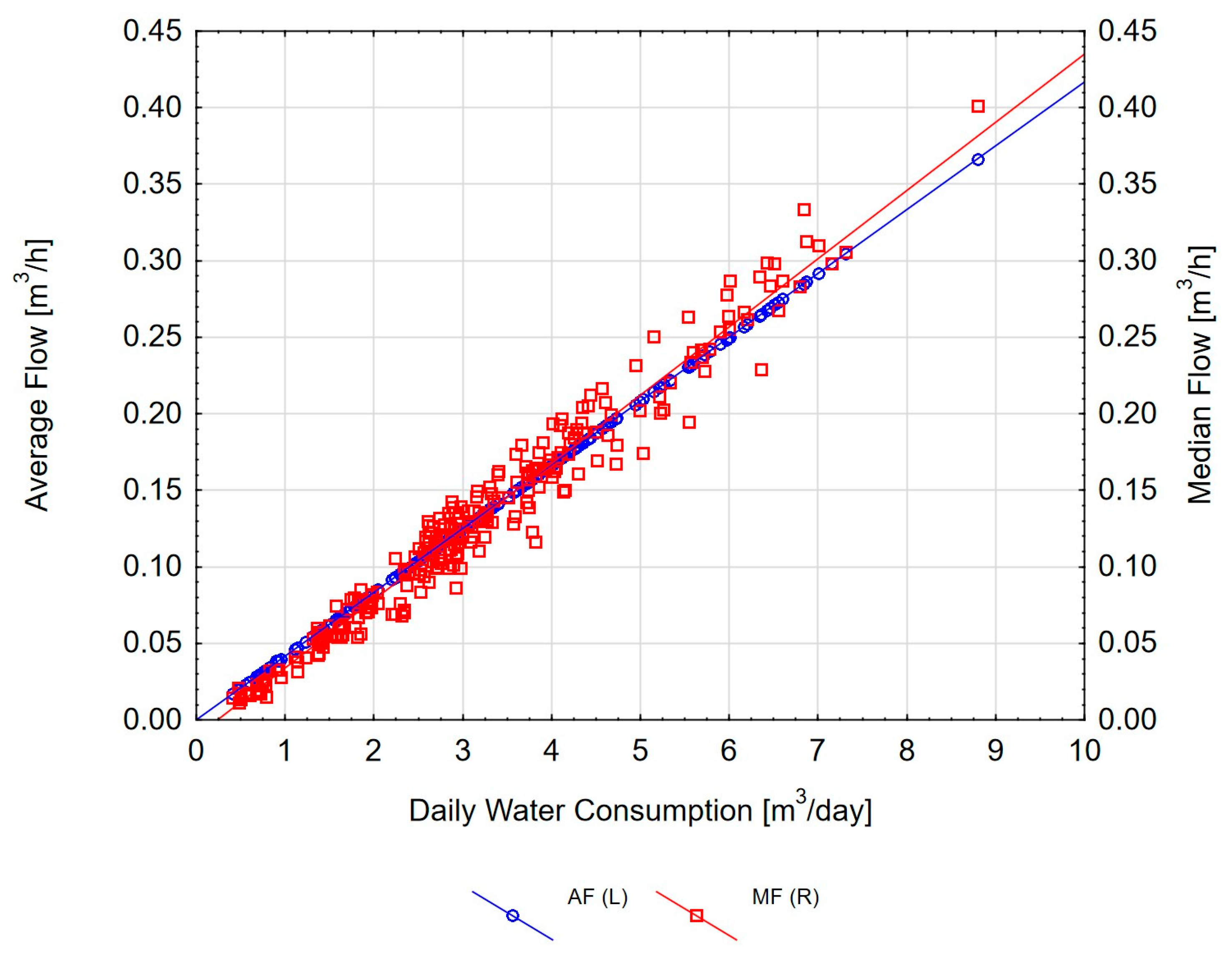
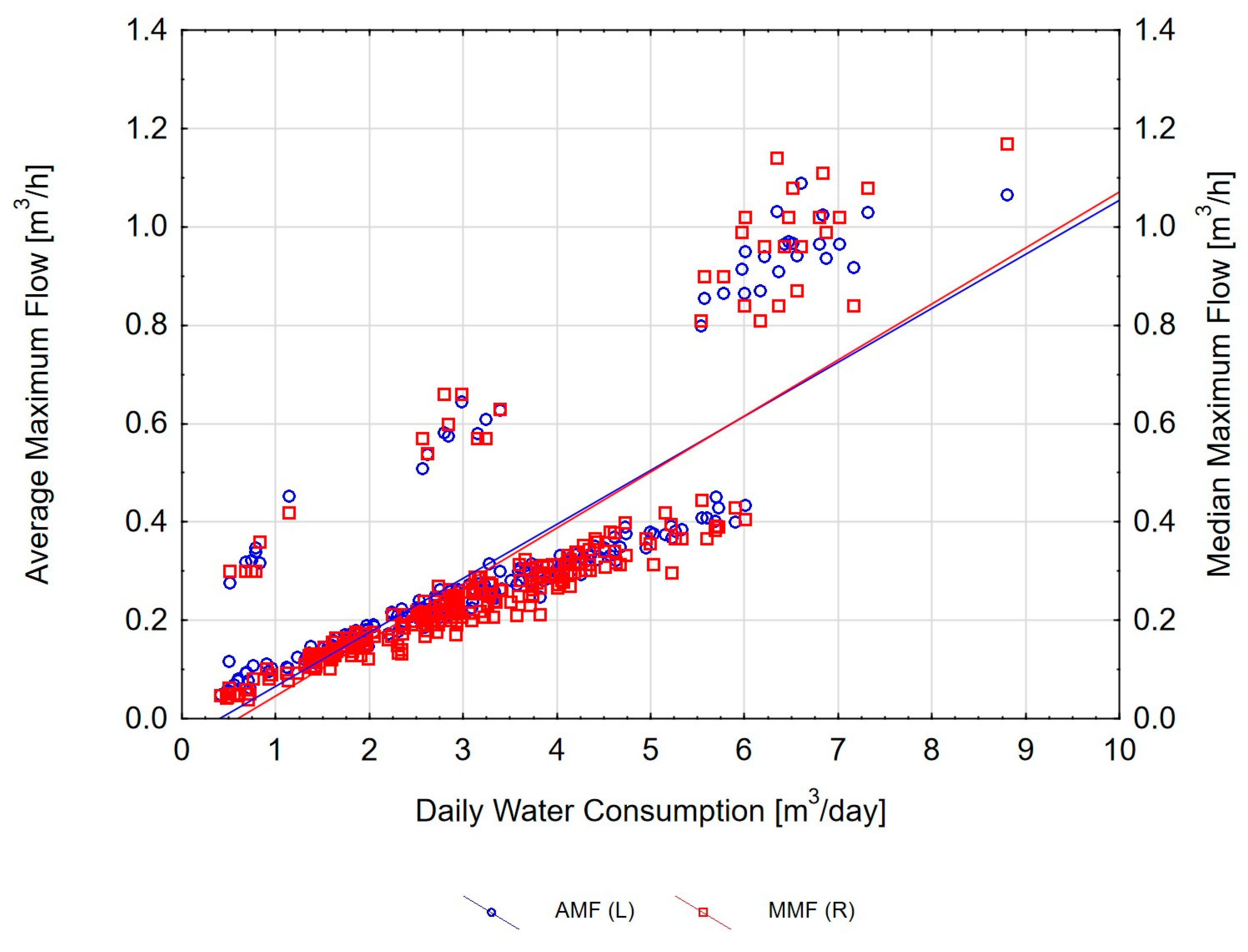
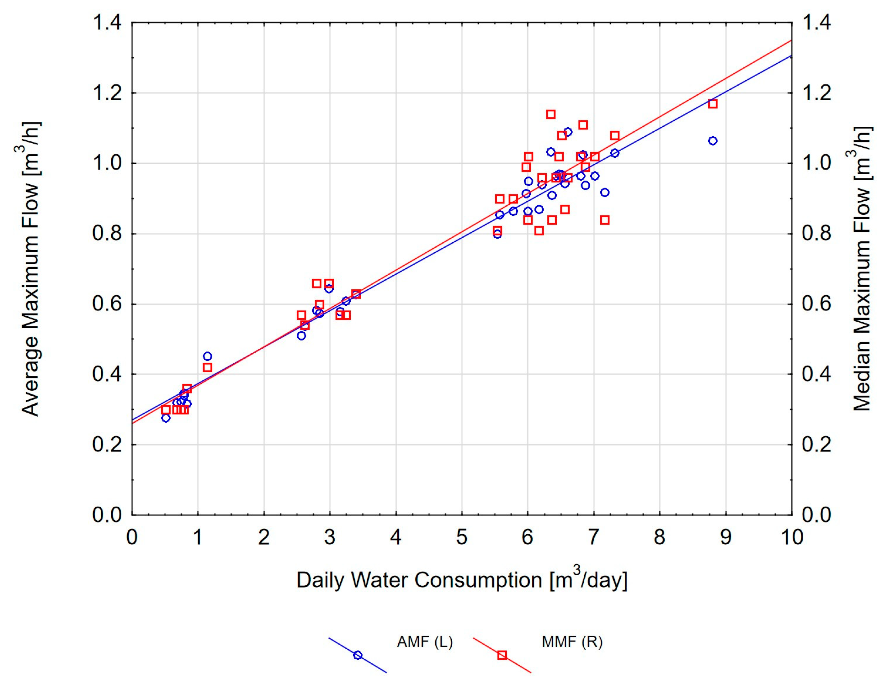
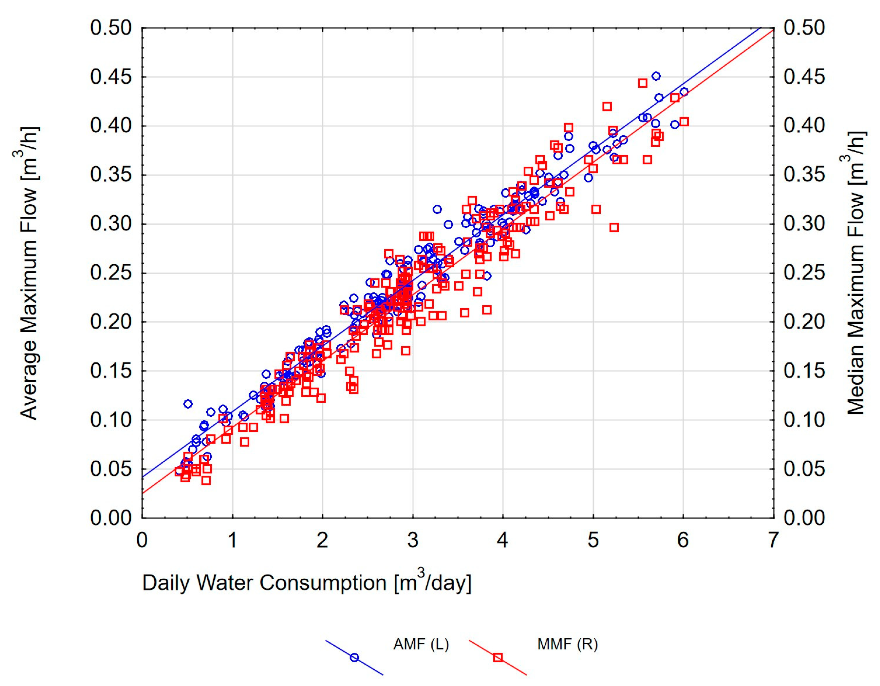
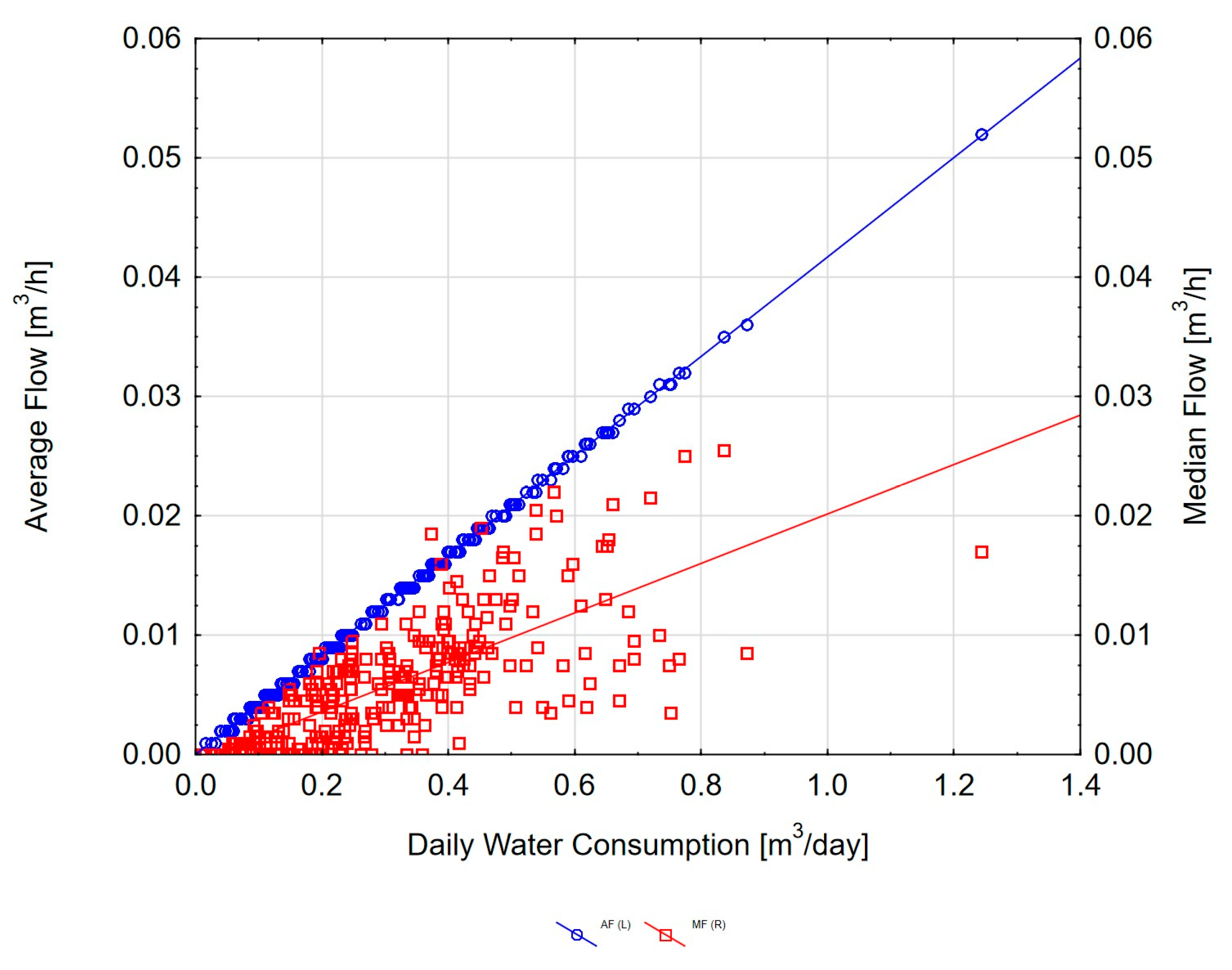
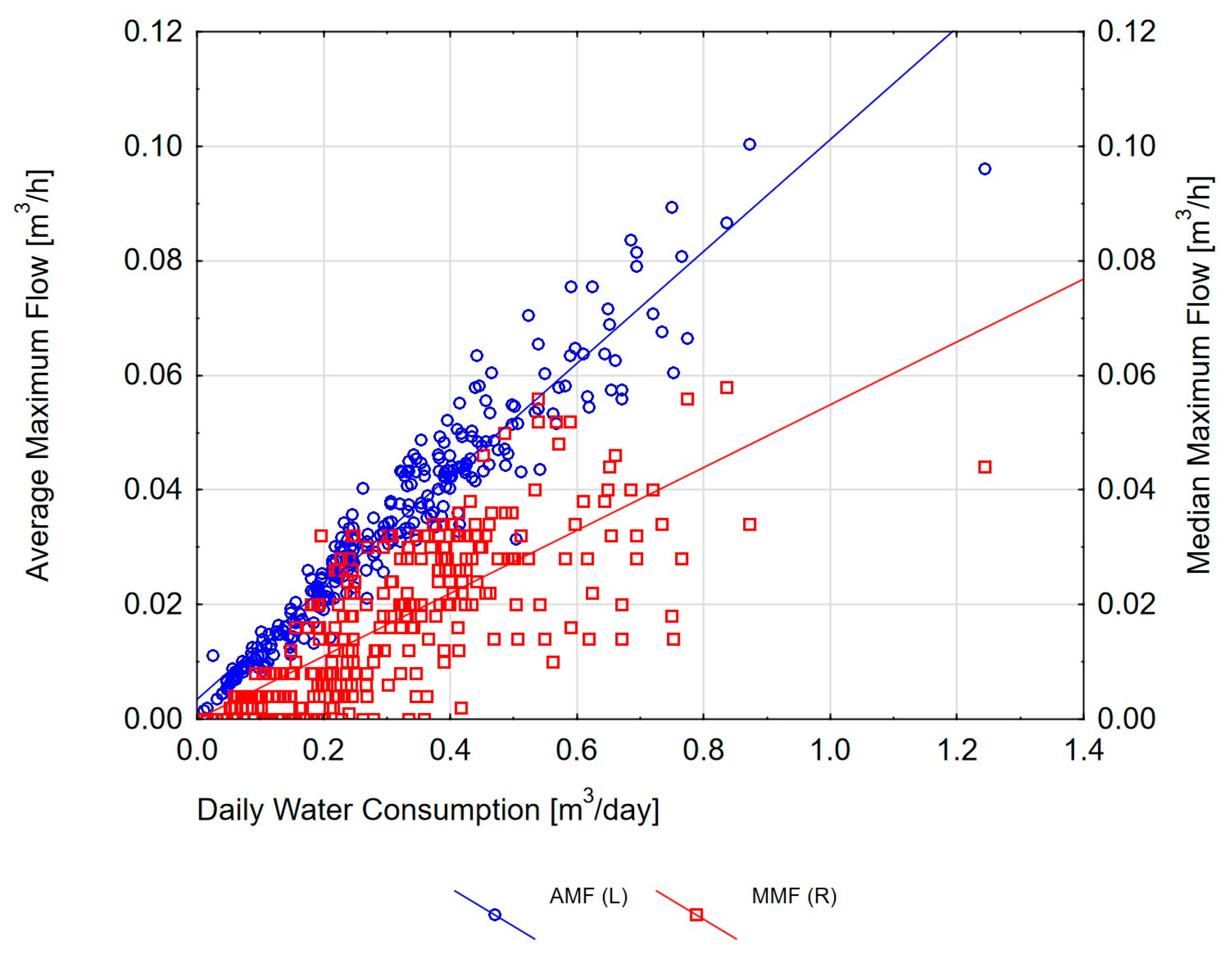
3.2. Dependence of Characteristic Flows on Daily Water Consumption in the Building

The next step of the research was to analyze the relationship between the hourly flow values and the daily consumption values. Figure 5 presents the dependence of the value of the average hourly flow (AF) and the median of the average hourly flows (MF) on the daily water consumption (DWC) in multi-family buildings. The value of the correlation coefficient of MF concerning DWC is r = 0.9800.

Figure 6 presents the relationships between average maximum flow (AMF) concerning DWC and median maximum flow (MMF) concerning DWC in multi-family buildings. Two groups of objects and relationships between flow values and consumption are visible. The correlation coefficient for all objects when analyzing AMF versus DWC is r = 0.8087, and the correlation of MMF values to DWC is r = 0.7955.

Due to the high values of the correlation coefficient, a mathematical model for determining the AMF based on the DWC value was developed:

$$AMF=0.110·DWC-0.043[{\mathrm{m}}^3/\mathrm{h}]$$

(2)

The average flow (AF) and median flow (MF) values are very close to each other. Due to the large distances of the observed values from the trend line, it was decided to separate both groups and evaluate them separately.

Figure 7 presents the AMF and MMF values relative to DWC in multi-family buildings for facilities above the trend line of all facilities. The correlation of AMF values with DWC was r = 0.9842. The correlation of MMF values with DWC was r = 0.9630.

Due to the high values of the correlation coefficient, a mathematical model was developed to determine the AMF based on the DWC value:

$$AMF=0.104·DWC+0.271[{\mathrm{m}}^3/\mathrm{h}]$$

(3)

Figure 8 presents the AMF and MMF values relative to DWC in multi-family buildings for facilities below the trend line of all facilities. The correlation of AMF values with DWC was r = 0.9842. The correlation of MMF values with DWC was r = 0.9614.

Due to the high values of the correlation coefficient, a mathematical model was developed to determine the AMF based on the DWC value:

$$AMF=0.669·DWC+0.042[{\mathrm{m}}^3/\mathrm{h}]$$

(4)

The correlation analysis of AMF and MMF values against DWC for all objects was close to the value of r = 0.80. In the individual groups of objects, this correlation increased to values above r = 0.96 in the case of the median and above 0.98 in the case of AMF.

The correlation results confirm the usefulness of the results obtained from multi-family buildings for further studies.

Figure 9 presents the dependence of the AF and MF on the daily water consumption in single-family buildings. The value of the correlation coefficient of MF concerning DWC is r = 0.9588, with a confidence of 0.95. The values of the median hourly flow deviate from the trend line as the daily consumption value increases. Single-family facilities with daily consumption of up to 0.4 m³/day constitute the majority of facilities (over 60%). This is typical for single-family buildings, which are usually inhabited by four people with a daily consumption of approximately 100 dm³/day/person [35,36,37].

Figure 10 presents a scatterplot of the average maximum hourly flow of daily water consumption in single-family buildings and the median value of the maximum flow of daily water consumption in single-family buildings. The correlation value of AMF concerning DWC is r = 0.9588 with a confidence of 0.95. The correlation value of MMF concerning DWC is r = 0.7434 with a confidence of 0.95.

Due to the high values of the correlation coefficient, a mathematical model was developed to determine the AMF based on the DWC value:

$$AMF=0.098·DWC+0.003[{\mathrm{m}}^3/\mathrm{h}]$$

(5)

The obtained correlation results confirm the usefulness of the results obtained from single-family buildings for further studies.

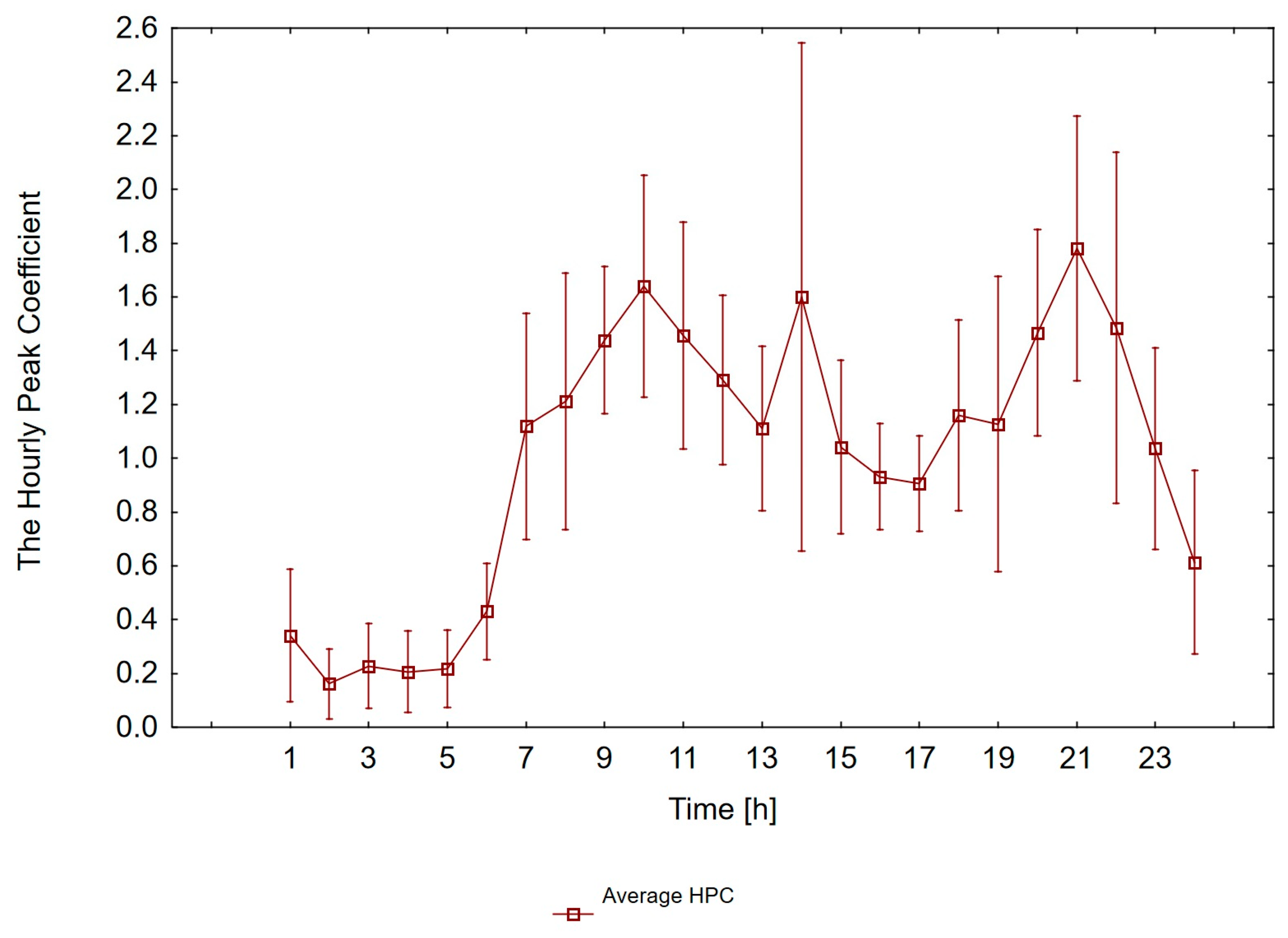
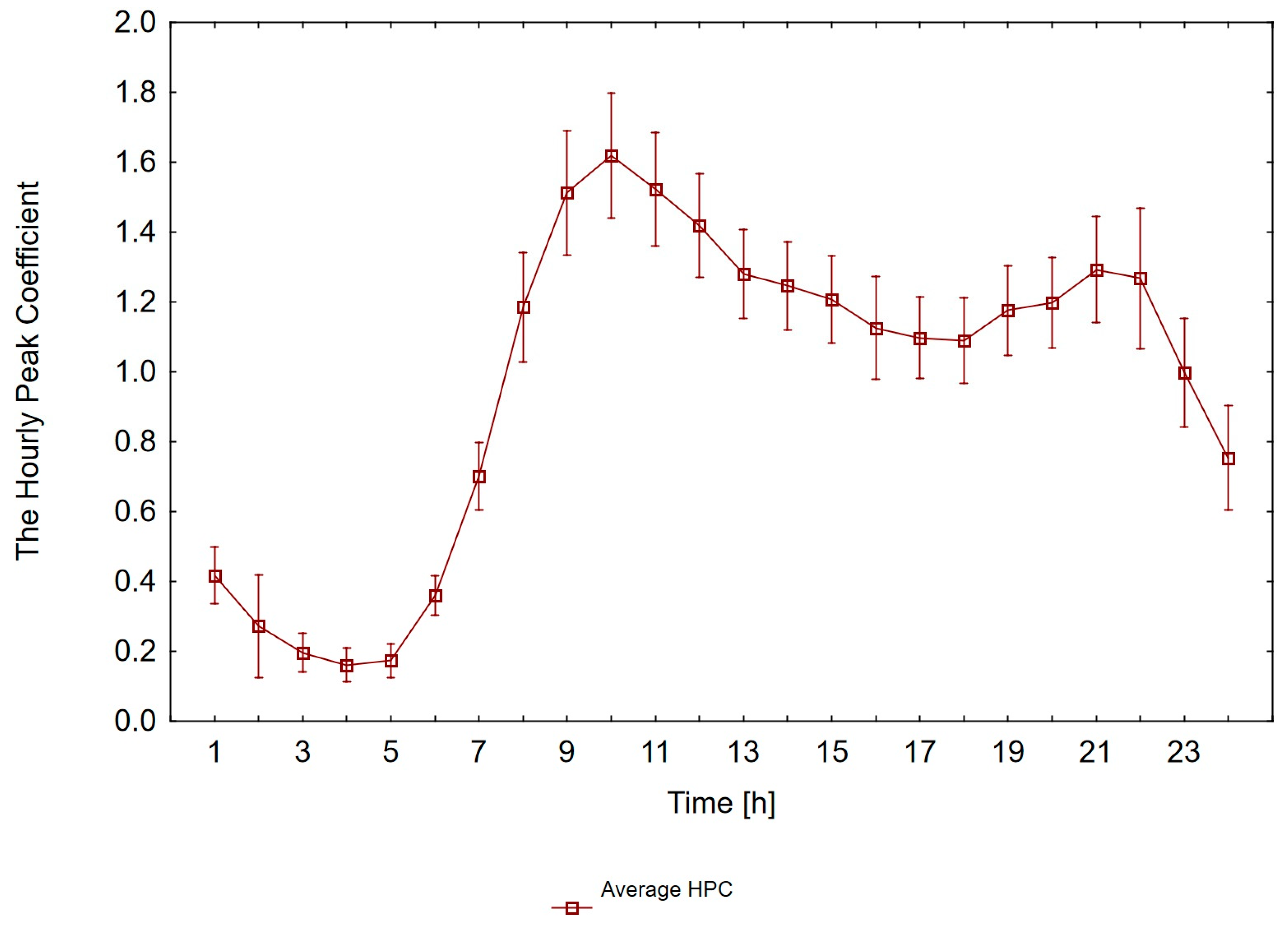
3.3. The Hourly Peak Coefficient

The last stage of the research was to develop a common characteristic of daily water consumption and to determine the scope of HPC changes at particular hours of the day. Two characteristics were obtained: single-family buildings and multi-family buildings. Figure 11 presents the demand pattern for single-family properties. There are three periods of increased water consumption typical of single-family buildings: morning, lunchtime, and evening. The average HPC value varies from 0.18 at night to 1.80 at the time of maximum water consumption. Between 00:00 and 05:00 and from 15:00 to 16:00, HPC values change the least in individual facilities. The greatest changes in the HPC value occur at 1:00 p.m., where the HPC varies from 0.60 to over 2.40. Depending on the building, the consumption curve is then characterized by two or three periods of maximum water consumption. Another hour with very high variability is 9:00 p.m., where HPC changes range from 0.8 to over 2.0 AF values. Large changes also occur at 6:00 a.m., 7:00 a.m., 6:00 p.m., and 8:00 p.m., where the differences between HPC min. given hour and the HPC max is over 1.0. The HPC values at individual hours of the day in the examined facilities differ by more than ±40% compared to the HPC av for a given hour.

Figure 12 presents the demand pattern for multi-family buildings. There are two periods of increased water consumption typical of multi-family buildings: morning and evening. The average HPC value varies from 0.15 at night to 1.60 at the time of maximum water consumption. Variable average HPC values are lower than HPC values for single-family housing. In the hours from 02:00 to 05:00, HPCs change the least in individual facilities. The greatest changes in the HPC value occur at 9:00 p.m., where the HPC varies from 1.07 to over 1.49. The next hours with high variability are 08:00 and 09:00, where the HPC changes are 0.36 and 0.37 of the AF value, respectively. HPC values for individual hours in all facilities do not differ from the HPC avg by more than ±22%, and for most hours, they do not differ by more than ±10%.

The HPC values estimated on the basis of the measurements performed for both single-family buildings (average 1.80) and multi-family buildings (average 1.60) are much lower than the values given in the Polish design guidelines (3.5—single-family buildings, 1.8 to 2.5—multi-family buildings), which is also consistent with the results of other studies described in the Introduction section.

4. Conclusions

The authors conducted field tests of single-family and multi-family buildings in the field of monitoring water consumption and characteristics of water consumption during the day. Analyses of the relationship between AF, MF, AMF, and MMF about DWC were carried out, and four mathematical models were obtained to determine the maximum flow value based on the expected daily consumption in the building: one model for single-family buildings and three models for multi-family buildings.

These models can support the process of selecting water meters in single-family and multi-family buildings in the diameter range of DN15-DN40.

As part of the HPC analysis, two characteristics of variations in water consumption during the day were obtained for multi-family buildings and single-family buildings. The obtained characteristics can be used for

• The process of selecting water meters by determining the expected minimum and maximum flows during the day depending on the average daily flow;
• The characteristics can be used for the process of building hydraulic models of water distribution systems and for calibrating the models, indicating the scope of HPC modifications for facilities.

The values of HPC indicators are comparable to the literature values achieved in other studies in Poland and Italy, as well as Mexico.

The research and analyses carried out and the results obtained in the form of formulas and characteristics demonstrate scientific and implementation value, supporting engineers responsible for water meters management and optimization and modernization works of the water supply system.

The research conducted by the authors concerns continuous water supply systems. There are no intermittent water supply systems in Poland. Carrying out research for an intermittent water supply system would be an interesting experience and would develop the topic of determining consumption curves and selecting appropriate measurement arrangements.

References

1. Lee, S.; Kim, J.H. Quantitative Measure of Sustainability for Water Distribution Systems: A Comprehensive Review. Sustainability 2020, 12, 10093. [Google Scholar] [CrossRef]
2. Borzì, I. Evaluating Sustainability Improvement of Pressure Regime in Water Distribution Systems Due to Network Partitioning. Water 2022, 14, 1787. [Google Scholar] [CrossRef]
3. Giudicianni, C.; Herrera, M.; di Nardo, A.; Adeyeye, K. Automatic Multiscale Approach for Water Networks Partitioning into Dynamic District Metered Areas. Water Resour. Manag. 2020, 34, 835–848. [Google Scholar] [CrossRef]
4. Price, E.; Abhijith, G.R.; Ostfeld, A. Pressure Management in Water Distribution Systems through PRVs Optimal Placement and Settings. Water Res. 2022, 226, 119236. [Google Scholar] [CrossRef] [PubMed]
5. Grigg, N.S. Water Distribution Systems: Integrated Approaches for Effective Utility Management. Water 2024, 16, 524. [Google Scholar] [CrossRef]
6. Alcocer, Y.V.H.; Tzatchkov, V.G.; Buchberger, S.G.; Arreguin, F.I.; Feliciano, D. Stochastic Residential Water Demand Characterization. In Critical Transitions in Water and Environmental Resources Management; ASCE Library: Reston, VA, USA, 2012; pp. 1–10. [Google Scholar] [CrossRef]
7. Dadar, S.; Đurin, B.; Alamatian, E.; Plantak, L. Impact of the Pumping Regime on Electricity Cost Savings in Urban Water Supply System. Water 2021, 13, 1141. [Google Scholar] [CrossRef]
8. Annus, I.; Vassiljev, A. Different Approaches for Calibration of an Operational Water Distribution System Containing Old Pipes. Procedia Eng. 2015, 119, 526–534. [Google Scholar] [CrossRef]
9. Świętochowska, M.; Bartkowska, I. Analysis of Water Age and Flushing of the Water Supply Network of the Pressure Reduction Zone. J. Ecol. Eng. 2022, 23, 229–238. [Google Scholar] [CrossRef]
10. Arregui, F.; Cabrera, E.; Cobacho, R.; García-Serra, J. Reducing Apparent Losses Caused By Meters Inaccuracies. Water Pract. Technol. 2006, 1, wpt2006093. [Google Scholar] [CrossRef]
11. Cimorelli, L.; Covelli, C.; Molino, B.; Pianese, D. Optimal Regulation of Pumping Station in Water Distribution Networks Using Constant and Variable Speed Pumps: A Technical and Economical Comparison. Energies 2020, 13, 2530. [Google Scholar] [CrossRef]
12. Gutiérrez-Bahamondes, J.H.; Mora-Meliá, D.; Iglesias-Rey, P.L.; Martínez-Solano, F.J.; Salgueiro, Y. Pumping Station Design in Water Distribution Networks Considering the Optimal Flow Distribution between Sources and Capital and Operating Costs. Water 2021, 13, 3098. [Google Scholar] [CrossRef]
13. Świętochowska, M.; Bartkowska, I. Optimization of Energy Consumption in the Pumping Station Supplying Two Zones of the Water Supply System. Energies 2022, 15, 310. [Google Scholar] [CrossRef]
14. Szpak, D.; Tchórzewska-Cieślak, B.; Stręk, M. A New Method of Obtaining Water from Water Storage Tanks in a Crisis Situation Using Renewable Energy. Energies 2024, 17, 874. [Google Scholar] [CrossRef]
15. Gwoździej-Mazur, J.; Świętochowski, K. Non-Uniformity of Water Demands in a Rural Water Supply System. J. Ecol. Eng. 2019, 20, 245–251. [Google Scholar] [CrossRef]
16. Balacco, G.; Carbonara, A.; Gioia, A.; Iacobellis, V.; Piccinni, A.F. Evaluation of Peak Water Demand Factors in Puglia (Southern Italy). Water 2017, 9, 96. [Google Scholar] [CrossRef]
17. Ogiołda, E.; Nowogoński, I.; Pietrzak, P. Characteristics of Water Consumption in Chocianów, Parchów and Pogorzeliska, Lower Silesia Province. Civ. Environ. Eng. Rep. 2019, 29, 13–21. [Google Scholar] [CrossRef]
18. Ogiołda, E.; Kozaczek, M. Characteristics of Water Consumption in Water Supply Systems in “Wilków” and “Borek” in Głogów Commune. Zesz. Nauk. Uniw. Zielonogórskiego 2013, 32, 69–77. [Google Scholar]
19. Podwójci, P. Inequality of Water Consumption and Distribution in Apartment House Building. Ecol. Eng. 2011, 26, 281–289. [Google Scholar]
20. Hernandez-Samaniego, E.; Navarro-Gomez, C.; Sánchez, D.H.; Sánchez-Navarro, J.R. Coefficients and Curves of Hourly and Daily Variations of Water Demand for Improved Operation of Potable Water Distribution Systems: A Case Study of Chihuahua City, Mexico. Water Pract. Technol. 2023, 18, 1991–2001. [Google Scholar] [CrossRef]
21. Płoskonka, R.; Beńko, P. Daily changes of water demand in the single water system zone in Krakow. Czas. Tech. 2015, 2014, 35–43. [Google Scholar] [CrossRef]
22. Beal, C.D.; Stewart, R.A. Identifying Residential Water End Uses Underpinning Peak Day and Peak Hour Demand. J. Water Resour. Plan. Manag. 2014, 140, 04014008. [Google Scholar] [CrossRef]
23. Newfoundland and Labrador Department of Environment and Conservation; CBCL Limited. Study on Water Quality and Demand on Public Water Supplies with Variable Flow Regimes and Water Demand: Final Report; Newfoundland and Labrador Department of Environment and Conservation: St. John’s, NL, Canada, 2011.
24. Tkaczukowa, B.; Nowakowska-Błaszczyk, A. Guidelines for Determining Water Demand and Sewage Production in Towns; Institute of Spatial and Municipal Management (Instytut Gospodarki Przestrzennej i Komunalnej): Warsaw, Poland, 1991. (In Polish) [Google Scholar]
25. Burgschweiger, J.; Gnädig, B.; Steinbach, M.C. Optimization Models for Operative Planning in Drinking Water Networks. Optim. Eng. 2009, 10, 43–73. [Google Scholar] [CrossRef]
26. Lambert, A.O.; Brown, T.G.; Takizawa, M.; Weimer, D. A Review of Performance Indicators for Real Losses from Water Supply Systems. J. Water Supply Res. Technol.-AQUA 1999, 48, 227–237. [Google Scholar] [CrossRef]
27. Farley, M.; Wyeth, G.; Ghazali, Z.B.M.; Istandar, A.; Singh, S. The Manager’s Non-Revenue Water Handbook: A Guide to Understanding Water Losses; United States Agency for International Developing and Ranhill Utilities: Waszyngton, DC, USA, 2008. [Google Scholar]
28. Directive-2014/32-EN-EUR-Lex. Available online: https://eur-lex.europa.eu/legal-content/EN/TXT/?uri=CELEX:32014L0032 (accessed on 15 March 2024).
29. Announcement of the Speaker of the Sejm of the Republic of Poland of 10 March 2023 on the Announcement of the Uniform Text of the Construction Law Act. Available online: https://isap.sejm.gov.pl/isap.nsf/download.xsp/WDU20230000682/T/D20230682L.pdf (accessed on 3 April 2024).
30. Gwoździej-Mazur, J. Monitoring of Water Supply Connections as an Element to Reduce Apparent Losses of Water? E3S Web Conf. 2017, 22, 00061. [Google Scholar] [CrossRef]
31. Mambretti, S.; Brebbia, C.A. Urban Water; WIT Press: Southampton, UK, 2012; ISBN 978-1-84564-576-2. [Google Scholar]
32. Tricarico, C.; de Marinis, G.; Gargano, R.; Leopardi, A. Peak Residential Water Demand. Proc. Inst. Civ. Eng.-Water Manag. 2007, 160, 115–121. [Google Scholar] [CrossRef]
33. Walski, T.; Chase, D.; Savic, D.; Grayman, W.; Backwith, S.; Koelle, E. Advanced Water Distribution Modeling and Management; Haestad Press: Waterbury, CT, USA, 2003. [Google Scholar]
34. Balacco, G.; Gioia, A.; Iacobellis, V.; Piccinni, A.F. At-Site Assessment of a Regional Design Criterium for Water-Demand Peak Factor Evaluation. Water 2019, 11, 24. [Google Scholar] [CrossRef]
35. Myka-Raduj, A.; Jóźwiakowski, K.; Siwiec, T.; Raduj, W. Changes of Water Consumption in a Forester’s Lodge in Polesie National Park (Poland)—Case Study. Water 2023, 15, 3157. [Google Scholar] [CrossRef]
36. Bergel, T.; Kaczor, G.; Bugajski, P. Analysis of the Structure of Water Consumption in Rural Households in Terms of Design Guidelines Water and Sewage Systems. Infrastrukt. Ekol. Teren. Wiej. 2016, nr IV/4, 1899–1910. [Google Scholar] [CrossRef]
37. Pawełek, J.; Bergel, T.; Woyciechowska, O. Variation in Water Consumption in Rural Households during the Multi-Year Period. Acta Sci. Pol. Form. Circumiectus 2016, 14, 85–94. [Google Scholar] [CrossRef]
Figure 1. The figure shows the locations of the research facilities (towns).
Water 16 01077 g001
Figure 2. The figure shows photos of the field research: (1). measuring sets ready for installation; (2). a measuring set installed on the connection of a single-family house; (3). a measuring set—water meter DN20 mounted on the connection of a multi-family house; (4). a measuring set—water meter DN40 mounted on the connection of a multi-family house.
Water 16 01077 g002
Figure 3. The figure contains graphs showing the obtained water consumption curves on individual test days for sample single-family buildings.
Water 16 01077 g003
Figure 4. The figure contains graphs showing the obtained water consumption curves on individual test days for sample multi-family buildings.
Water 16 01077 g004
Figure 5. The figure shows a scatter chart of the average hourly flow values and the median flow values against daily water consumption in multi-family buildings.
Water 16 01077 g005
Figure 6. The figure shows a scatter chart of the value of the average maximum hourly flow against the daily water consumption in multi-family buildings and the value of the median maximum flow against the daily water consumption in multi-family buildings—all facilities.
Water 16 01077 g006
Figure 7. The figure shows a scatterplot of the average maximum hourly flow values against daily water consumption in multi-family buildings and the median maximum flow values against daily water consumption in multi-family buildings above the trend lines.
Water 16 01077 g007
Figure 8. The figure shows a scatterplot of the average maximum hourly flow about daily water consumption in multi-family buildings and the median value of maximum flow about daily water consumption in multi-family buildings below the trend lines.
Water 16 01077 g008
Figure 9. The figure shows a scatter chart of average hourly flow values against daily water consumption in single-family buildings and median flow values against daily water consumption in single-family buildings.
Water 16 01077 g009
Figure 10. The figure shows a scatter chart of the value of the average maximum hourly flow against the daily water consumption in single-family buildings and the value of the median maximum flow against the daily water consumption in single-family buildings.
Water 16 01077 g010
Figure 11. The figure shows the daily distribution curve in single-family buildings and the range of the peak hourly coefficient values in each hour.
Water 16 01077 g011
Figure 12. The figure shows the daily distribution curve in multi-family buildings and the range of the peak hourly coefficient values in each hour.
Water 16 01077 g012