
Investigation of the Tunnel Water Inflow Prediction Method Based on the MODFLOW-DRAIN Module


Abstract
1. Introduction
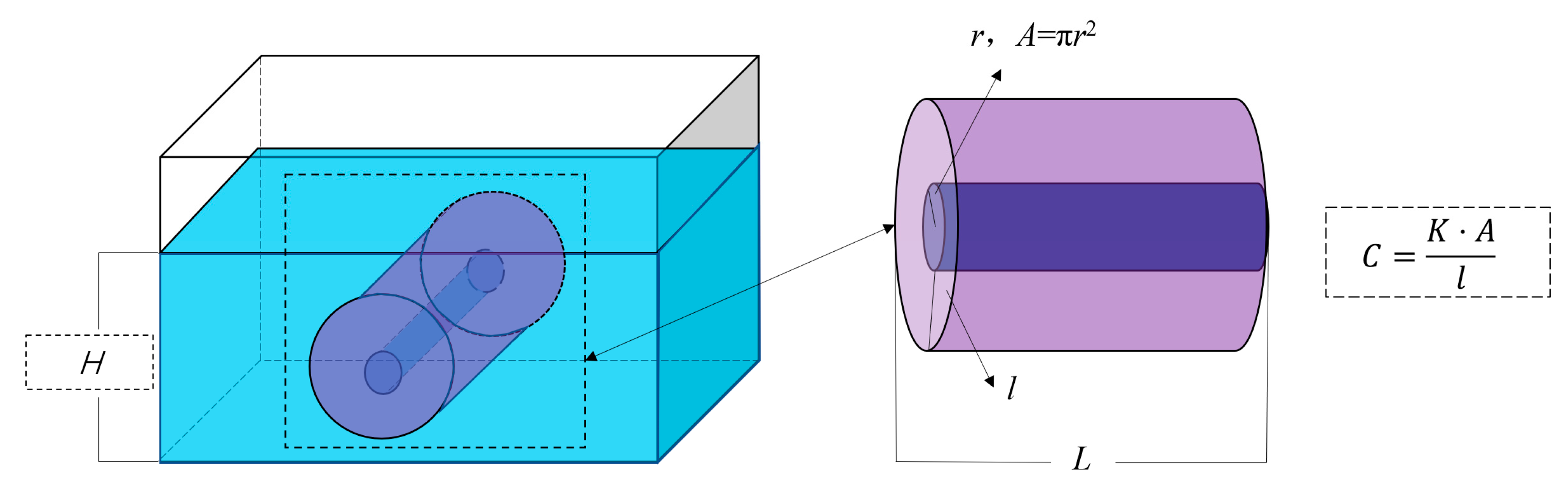
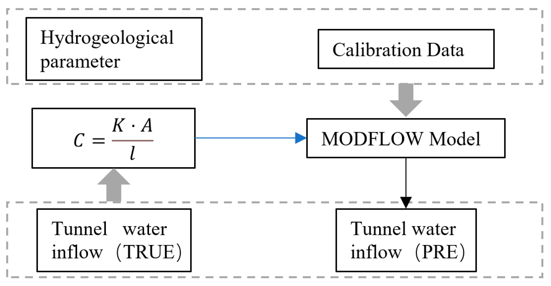
2. Theoretical Research
3. Case Analysis
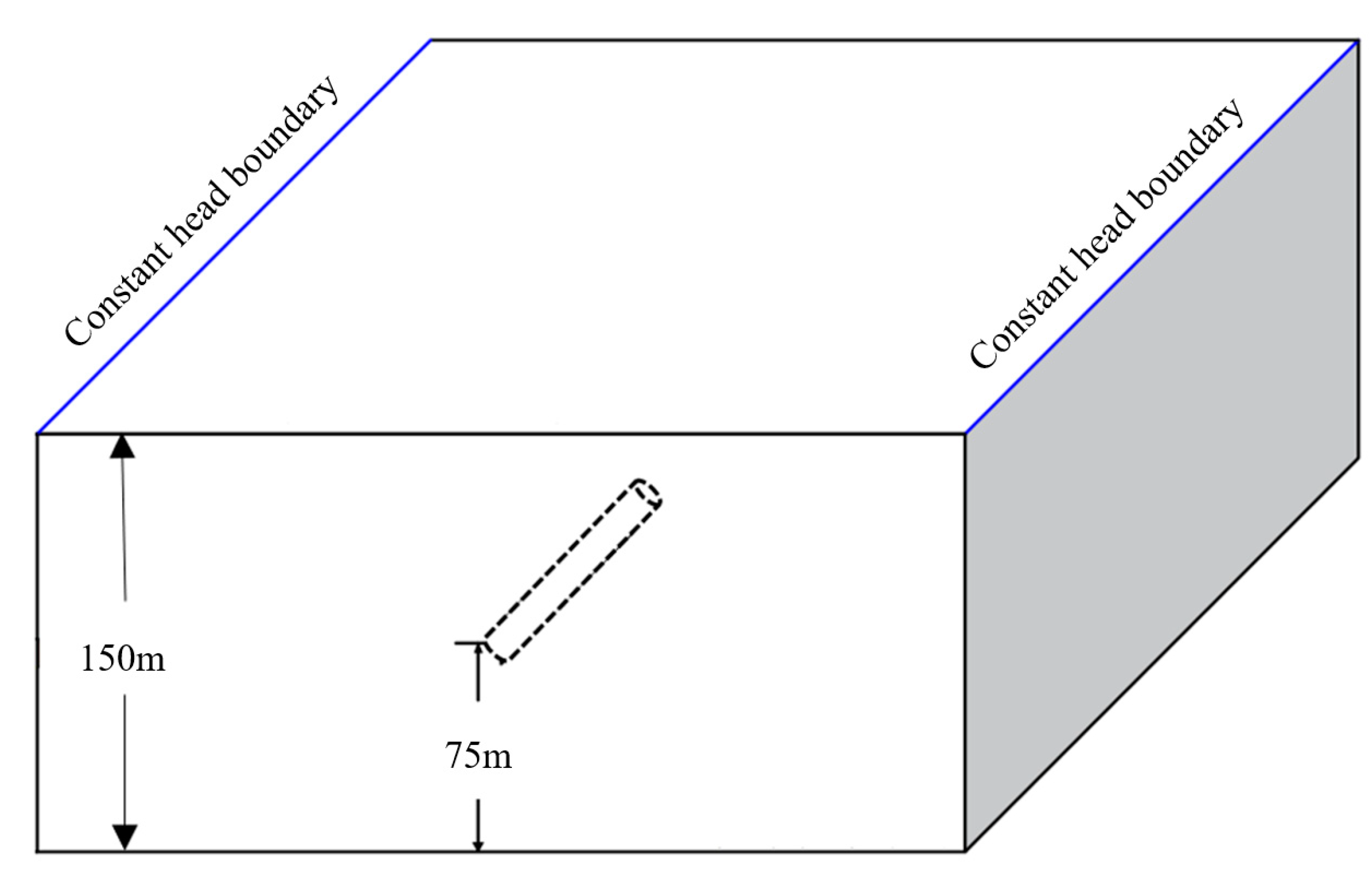
3.1. Study Settings
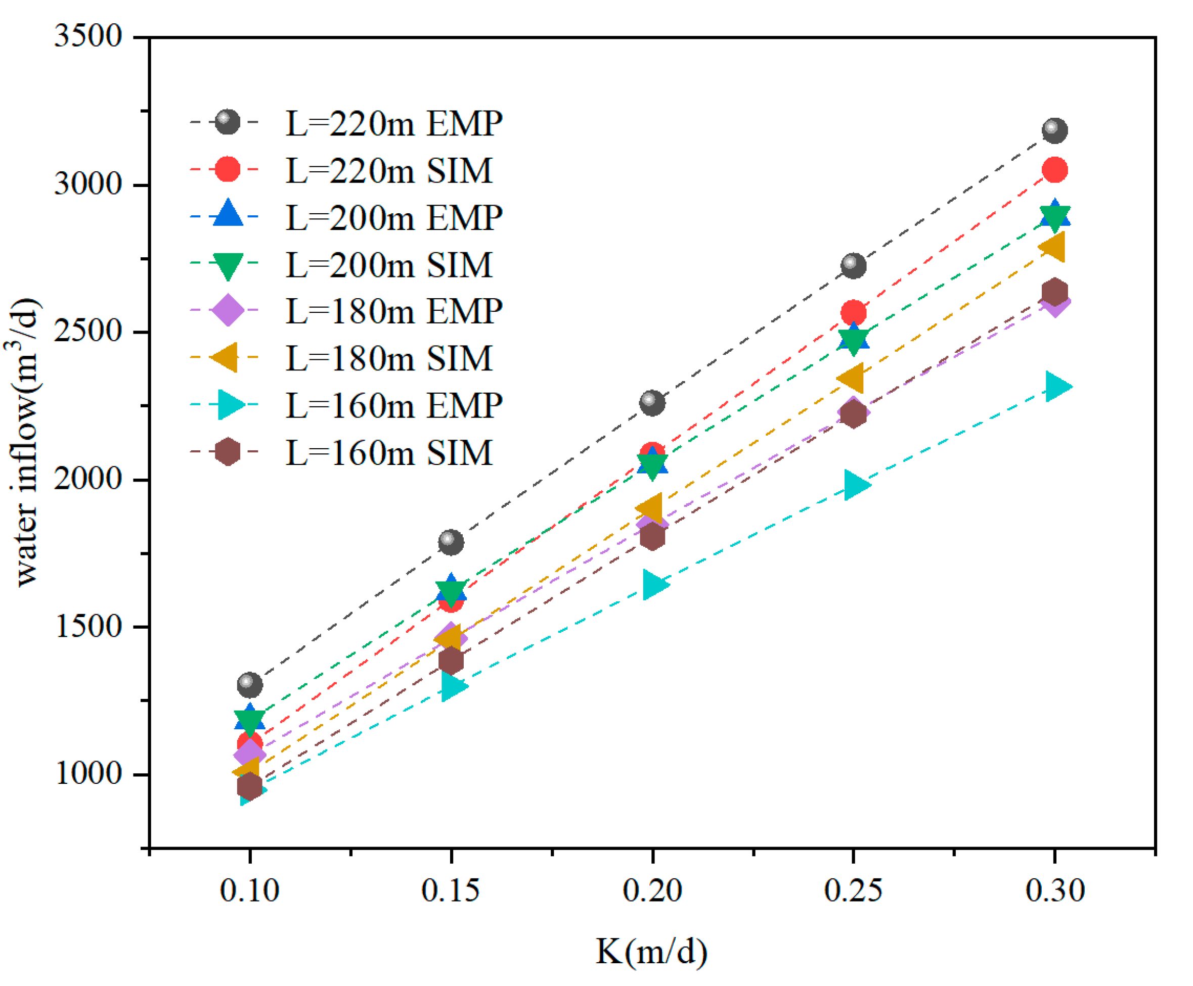
3.2. Calculation Results
3.3. Discussion
4. Engineering Case Study
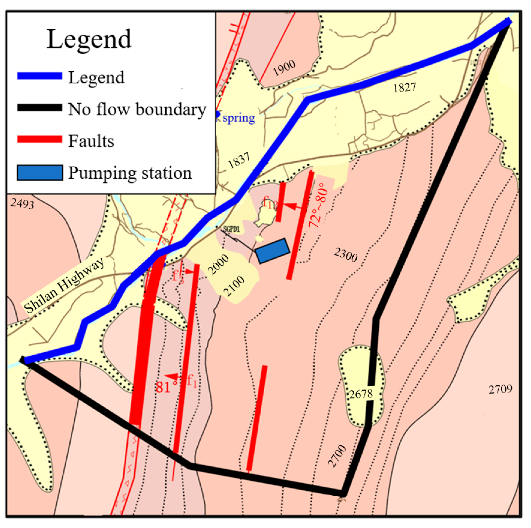
4.1. Project Introduction
4.2. Instance Model Parameter Settings
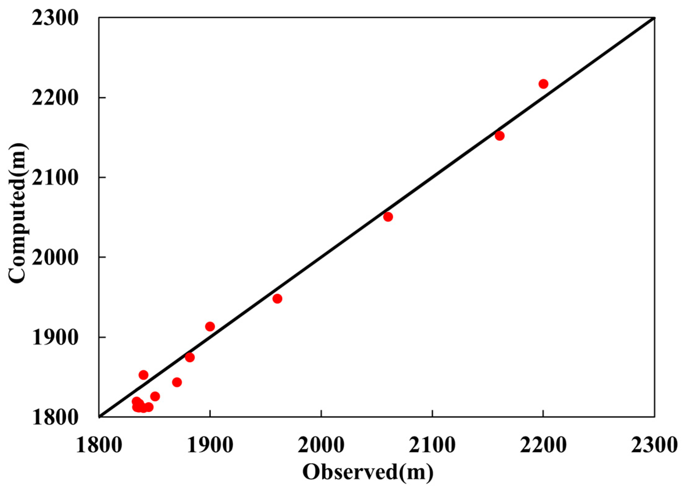
4.3. Model Calibration
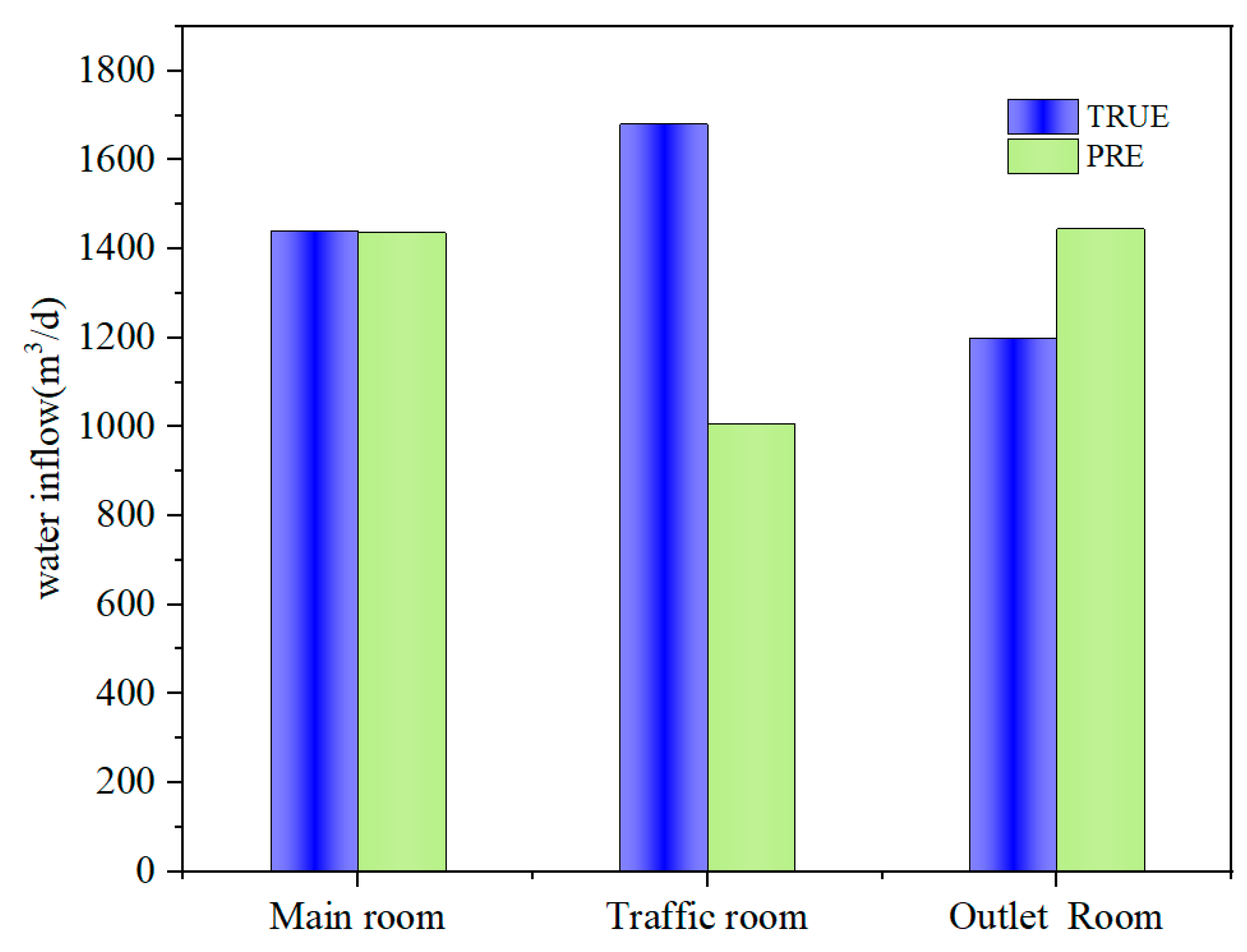
4.4. Water Inflow Prediction Results
5. Conclusions
- (1)
- The article delineates the physical significance and valuation method for key parameters within the DRAIN module, highlighting its accuracy in estimating water inflow volumes for typical drop tunnels. The drainage coefficient (C) value, tied to the permeability coefficient of the surrounding rock and the influence area’s definition, is calculable from the rock’s thickness post-excavation, equating to twice the tunnel’s radius. Ideally, the method’s results should closely align with empirical formulas, with discrepancies not surpassing 10%.
- (2)
- Practical applications of the method yield promising outcomes, with the article outlining procedural steps and considerations for its application. It presents a swift, efficient and effective numerical approach for tunnel water inflow estimation, laying a solid foundation for seepage control and enhancing tunnel construction safety.
Author Contributions
Funding
Data Availability Statement
Acknowledgments
Conflicts of Interest
References
- Chen, J.; Zhang, W.; Ma, J.; Zeng, B.; Huang, Y. An analytical approach to study the reinforcement performance of rock anchors. Eng. Fail. Anal. 2024, 160, 108200. [Google Scholar] [CrossRef]
- Katibeh, H.; Aalianvari, A. Development of a New Method for Tunnel Site Rating from. J. Appl. Sci. 2009, 9, 1496–1502. [Google Scholar] [CrossRef]
- Zarei, H.; Uromeihy, A.; Sharifzadeh, M. A new tunnel inflow classification (TIC) system through sedimentary rock masses. Tunn. Undergr. Space Technol. 2013, 34, 1–12. [Google Scholar] [CrossRef]
- Hwang, J.-H.; Lu, C.-C. A semi-analytical method for analyzing the tunnel water inflow. Tunn. Undergr. Space Technol. 2007, 22, 39–46. [Google Scholar] [CrossRef]
- Kolymbas, D.; Wagner, P. Groundwater ingress to tunnels–the exact analytical solution. Tunn. Undergr. Space Technol. 2007, 22, 23–27. [Google Scholar] [CrossRef]
- Maréchal, J.-C.; Perrochet, P. New analytical solution for the study of hydraulic interaction between Alpine tunnels and groundwater. Bull. Soc. Geol. Fr. 2003, 174, 441–448. [Google Scholar] [CrossRef]
- Perrochet, P. A simple solution to tunnel or well discharge under constant drawdown. Hydrogeol. J. 2005, 13, 886–888. [Google Scholar] [CrossRef]
- Verruijt, A. A complex variable solution for a deforming circular tunnel in an elastic half-plane. Int. J. Numer. Anal. Methods Geomech. 1997, 21, 77–89. [Google Scholar] [CrossRef]
- Park, K.-H.; Owatsiriwong, A.; Lee, J.-G. Analytical solution for steady-state groundwater inflow into a drained circular tunnel in a semi-infinite aquifer: A revisit. Tunn. Undergr. Space Technol. 2008, 23, 206–209. [Google Scholar] [CrossRef]
- Gattinoni, P.; Scesi, L. An empirical equation for tunnel inflow assessment: Application to sedimentary rock masses. Hydrogeol. J. 2010, 18, 1797–1810. [Google Scholar] [CrossRef]
- Farhadian, H.; Nikvar Hassani, A.; Katibeh, H. Groundwater inflow assessment to Karaj Water Conveyance tunnel, northern Iran. KSCE J. Civ. Eng. 2017, 21, 2429–2438. [Google Scholar] [CrossRef]
- Farhadian, H.; Katibeh, H.; Huggenberger, P.; Butscher, C. Optimum model extent for numerical simulation of tunnel inflow in fractured rock. Tunn. Undergr. Space Technol. 2016, 60, 21–29. [Google Scholar] [CrossRef]
- Farhadian, H.; Katibeh, H.; Huggenberger, P. Empirical model for estimating groundwater flow into tunnel in discontinuous rock masses. Environ. Earth Sci. 2016, 75, 471. [Google Scholar] [CrossRef]
- Shi, M.; Hu, W.; Li, M.; Zhang, J.; Song, X.; Sun, W. Ensemble regression based on polynomial regression-based decision tree and its application in the in-situ data of tunnel boring machine. Mech. Syst. Signal Process. 2023, 188, 110022. [Google Scholar] [CrossRef]
- Dai, Z.; Li, X.; Lan, B. Three-dimensional modeling of tsunami waves triggered by submarine landslides based on the smoothed particle hydrodynamics method. J. Mar. Sci. Eng. 2023, 11, 2015. [Google Scholar] [CrossRef]
- Tisler, W.; Szymkiewicz, A. Air trapping problem during infiltration on the large areas. In Proceedings of the 10th Conference on Interdisciplinary Problems in Environmental Protection and Engineering EKO-DOK 2018, Polanica-Zdrój, Poland, 16–18 April 2018. [Google Scholar]
- Guo, Y.F.; Wang, H.N.; Jiang, M.J. Efficient Iterative Analytical Model for Underground Seepage around Multiple Tunnels in Semi-Infinite Saturated Media. J. Eng. Mech. 2021, 147, 04021101. [Google Scholar] [CrossRef]
- Zhang, K.; Xue, Y.G.; Xu, Z.H.; Su, M.X.; Qiu, D.H.; Li, Z.Q. Numerical study of water inflow into tunnels in stratified rock masses with a dual permeability model. Environ. Earth Sci. 2021, 80, 260. [Google Scholar] [CrossRef]
- Zhao, X.; Yang, X.H. Experimental study on water inflow characteristics of tunnel in the fault fracture zone. Arab. J. Geosci. 2019, 12. [Google Scholar] [CrossRef]
- Tong, S.; Dong, Y.; Wang, L. Methods and applications of an unstructured grid version of MODFLOW: MODFLOW-USG. Hydrogeol. Eng. Geol. 2016, 43, 9–16. [Google Scholar]
- Ju, Q.; Hao, Z.; Yu, Z.; Chen, X.; She, C. Study of the Model of Spring Flow ForecastA Case Study of the Xiaonanhai Spring Catchement. J. Sichuan Univ. Eng. Sci. Ed. 2011, 43, 77–82. [Google Scholar]
- Qingyong, W.; Zhonghua, J.I.A.; Xiaofeng, L.I.U.; Feng, S.H.I. Visual MODFLOW and its application to groundwater simulation. J. Water Resour. Water Eng. 2007, 18, 90–92. [Google Scholar]
- Xia, Q. Characteristics of Error in Numerical Modeling of Well Flow with MODFLOW. Geotech. Investig. Surv. 2007, 37, 29–32. [Google Scholar]
- Reimann, T. MODFLOW-2005 CFP—A hybrid model for karst aquifers. Grundwasser 2009, 14, 139–145. [Google Scholar] [CrossRef]
- Zhang, B.; Hong, M.; Zou, Z.H.; Yeh, T.C.J.; Cheng, P. Embedding isochronous cells overland flow module into MODFLOW. Hydrol. Process. 2013, 27, 3833–3841. [Google Scholar] [CrossRef]
- Cheng, T.P.; Shao, J.L.; Cui, Y.L.; Mo, Z.Y.; Han, Z.; Li, L. Parallel simulation of groundwater flow in the North China Plain. J. Earth Sci. 2014, 25, 1059–1066. [Google Scholar] [CrossRef]
- Zhao, S.; Sun, S. Application of MODFLOW in Simulating Groundwater Seepage Flowing Field of Tiantai Landslide in Sichuan Province. J. Catastrophol. 2007, 22, 50–53. [Google Scholar]
- Raheem, A.; Ahmad, I.; Arshad, A.; Liu, J.P.; Rehman, Z.U.; Shafeeque, M.; Rahman, M.M.; Saifullah, M.; Iqbal, U. Numerical Modeling of Groundwater Dynamics and Management Strategies for the Sustainable Groundwater Development in Water-Scarce Agricultural Region of Punjab, Pakistan. Water 2024, 16, 34. [Google Scholar] [CrossRef]
- Sanaullah, M.; Wang, X.Q.; Ahmad, S.R.; Mirza, K.; Mahmood, M.Q.; Kamran, M. Optimized Irrigated Water Management Using Numerical Flow Modeling Coupled with Finite Element Model: A Case Study of Rechna Doab, Pakistan. Water 2023, 15, 4193. [Google Scholar] [CrossRef]
- Rubio-Arellano, A.B.; Ramos-Leal, J.A.; Vázquez-Báez, V.M.; Mora, J.I.R. Modeling the Groundwater Dynamics of the Celaya Valley Aquifer. Water 2023, 15, 1. [Google Scholar] [CrossRef]
- Li, W.; Zhang, B.; Hong, M.; Wang, B. Application of Visual MODFLOW in Assessment of Groundewater Resources in Longxi Area of Daqing. World Geol. 2003, 22, 161–165. [Google Scholar]
- Diaz, M.; Sinicyn, G.; Grodzka-Lukaszewska, M. Modelling of Groundwater-Surface Water Interaction Applying the Hyporheic Flux Model. Water 2020, 12, 3303. [Google Scholar] [CrossRef]
- Ostad, H.; Mohammadi, Z.; Fiorillo, F. Assessing the Effect of Conduit Pattern and Type of Recharge on the Karst Spring Hydrograph: A Synthetic Modeling Approach. Water 2023, 15, 1594. [Google Scholar] [CrossRef]
- Hunt, M.; Marandi, A.; Retike, I. Water Balance Calculation for a Transboundary Aquifer System between Estonia and Latvia. Water 2023, 15, 3327. [Google Scholar] [CrossRef]
- Xu, H.; Li, G.; Dong, Y.; Zhang, S.; Li, M. An approach for simulating planar flux based on MODFLOW. Geotech. Investig. Surv. 2011, 39, 37–39. [Google Scholar]
- Wei, Y.; Xu, M.; Liu, J. Visual Modflow software and analysis on its application potential in study hydrogeological conditions of metallogenesis of sandstone-type uranium deposits. Uranium Geol. 2003, 19, 53–57. [Google Scholar]
- Cheng, J. Analysis on Differences among Solutions by Different Equations in MODFLOW. Geotech. Investig. 2002, 32, 25–27. [Google Scholar]
- Dong, P.; Wang, X. Application and discussion of MODFLOW’s simulation to the seepage of free surface. Geotech. Investig. Surv. 2009, 37, 27–30. [Google Scholar]
- Ma, C.; Li, K.; Shi, L.; Zhao, S.; Xia, Z. Application of visual modflow in simulation of an opencast mine underground water. Environ. Eng. 2011, 29, 98–101. [Google Scholar]
- Shu, L.; Xu, Y.; Wu, P. Groundwater Flow Numeric Simulation Method Based on Uncertainties of MODFLOW Parameters. J. Jilin Univ. Earth Sci. Ed. 2017, 47, 1803–1809. [Google Scholar]
- Qin, J.; Du, T.Z.; Hao, Z.C.; Xu, H.Q.; Li, B.T. Integration of artificial neural networks with a numerical groundwater model for simulating spring discharge. In Proceedings of the Advances in Energy Science and Equipment Engineering, Guangzhou, China, 30–31 May 2015; pp. 1197–1201. [Google Scholar]
- Liu, D.; Si, G.; Zheng, J.; Yu, J.; Liu, Y.; Chen, J.; Ma, J. Numerical Simulation and Impact Assessment of a Groundwater Pollution Based on MODFLOW. Radiat. Prot. 2013, 33, 30–36. [Google Scholar]
- Batelaan, O.; De Smedt, F. SEEPAGE, a new MODFLOW DRAIN package. Ground Water 2004, 42, 576–588. [Google Scholar] [CrossRef] [PubMed]
- Rodriguez, L.B.; Cello, P.A.; Vionnet, C.A.; Goodrich, D. Fully conservative coupling of HEC-RAS with MODFLOW to simulate stream—Aquifer interactions in a drainage basin. J. Hydrol. 2008, 353, 129–142. [Google Scholar] [CrossRef]
- Golian, M.; Teshnizi, E.S.; Nakhaei, M. Prediction of water inflow to mechanized tunnels during tunnel-boring-machine advance using numerical simulation. Hydrogeol. J. 2018, 26, 2827–2851. [Google Scholar] [CrossRef]
- Sartirana, D.; Zanotti, C.; Rotiroti, M.; De Amicis, M.; Caschetto, M.; Redaelli, A.; Fumagalli, L.; Bonomi, T. Quantifying Groundwater Infiltrations into Subway Lines and Underground Car Parks Using MODFLOW-USG. Water 2022, 14, 4130. [Google Scholar] [CrossRef]
- Zhao, L.; Xia, R.; Yang, Y.; Shao, J.; Yi, L.; Wang, Z. Discussion and application of simulation methods for karst conduit flow based on MODFLOW. Carsologica Sin. 2017, 36, 346–351. [Google Scholar] [CrossRef]
- Bredihin, V.V.; Akulshin, A.A.; Vladimirovna, B.N.; Sergeevna, P.V. A method of calculating filtration rate of an infiltration water intake in kursk region. J. Appl. Eng. Sci. 2017, 15, 208–211. [Google Scholar] [CrossRef]
- Wu, J.; Zhou, Z.; Li, M.; Chen, M. Advance on the methods for predicting water inflow into tunnels. J. Eng. Geol. 2019, 27, 890–902. [Google Scholar] [CrossRef]


| Expression | Symbolic Meaning | |
|---|---|---|
| Jubouyi’s formula [48] | Q is the well water inflow (m3/d); K is the permeability coefficient of the phreatic aquifer (m/d; H is the thickness of the phreatic layer (m); S is the stable water level drop in the well (m); R is the radius of the funnel when stable (m); r is the radius of the well (m). | |
| Kuniaki Sato’s formula [49] | Qmax is the predicted maximum possible water inflow through the tunnel (m3/d); Q is the predicted stable water inflow through the tunnel (m3/d); K is the permeability coefficient of the rock mass (m/d); H0 is the static water level to the center of the equivalent circle of the tunnel cross-section distance (m); L is the length of the tunnel passing through the aquifer (m); r is the equivalent circle radius of the tunnel cross-section (m); H is the thickness of the water-bearing body (m); ε is the test coefficient (generally 12.8). | |
| Kosgakov’s formula [49] | Qs is the predicted stable water inflow of the tunnel (m3/d); K is the rock mass permeability coefficient (m/d); H0 is the distance from the static water level to the center of the equivalent circle of the tunnel cross-section (m); L is the length of the tunnel passing through the aquifer (m); r is the equivalent circle radius of the tunnel cross-section (m); R is the radius of influence of tunnel water inrush. |
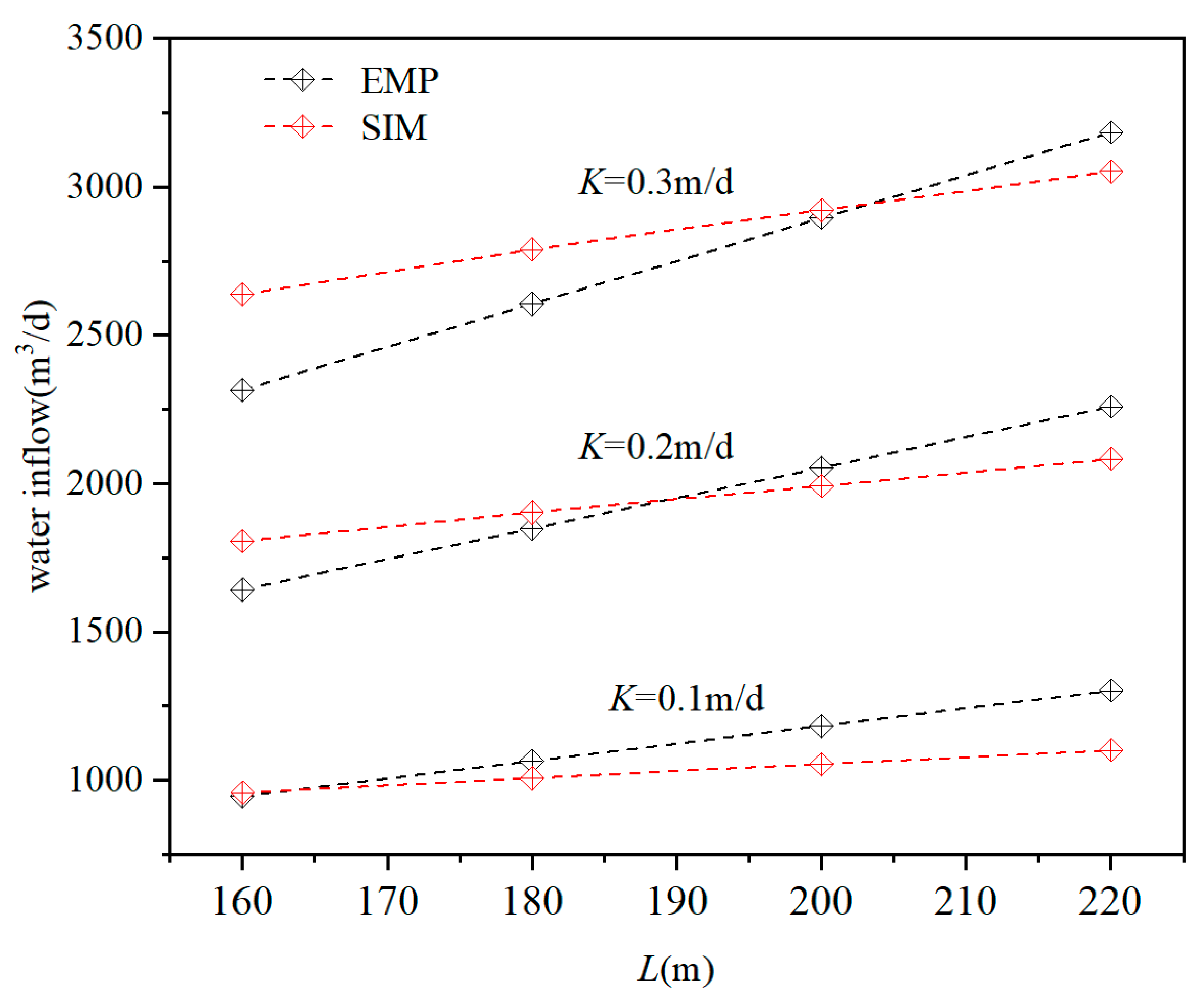
| K | L = 220 m | L = 200 m | L = 180 m | L = 160 m | ||||
|---|---|---|---|---|---|---|---|---|
| EMP | SIM | EMP | SIM | EMP | SIM | EMP | SIM | |
| 0.1 | 1303.20 | 1102.88 | 1184.72 | 1056.00 | 1066.25 | 1008.53 | 1066.25 | 1008.53 |
| 0.15 | 1787.12 | 1593.20 | 1624.66 | 1528.09 | 1462.19 | 1457.18 | 1462.19 | 1457.18 |
| 0.2 | 2259.82 | 2083.81 | 2054.38 | 1992.25 | 1848.94 | 1902.92 | 1848.94 | 1902.92 |
| 0.25 | 2724.69 | 2565.66 | 2476.99 | 2457.81 | 2229.29 | 2343.59 | 2229.29 | 2343.59 |
| 0.3 | 3183.63 | 3050.79 | 2894.21 | 2921.75 | 2604.79 | 2789.36 | 2604.79 | 2789.36 |
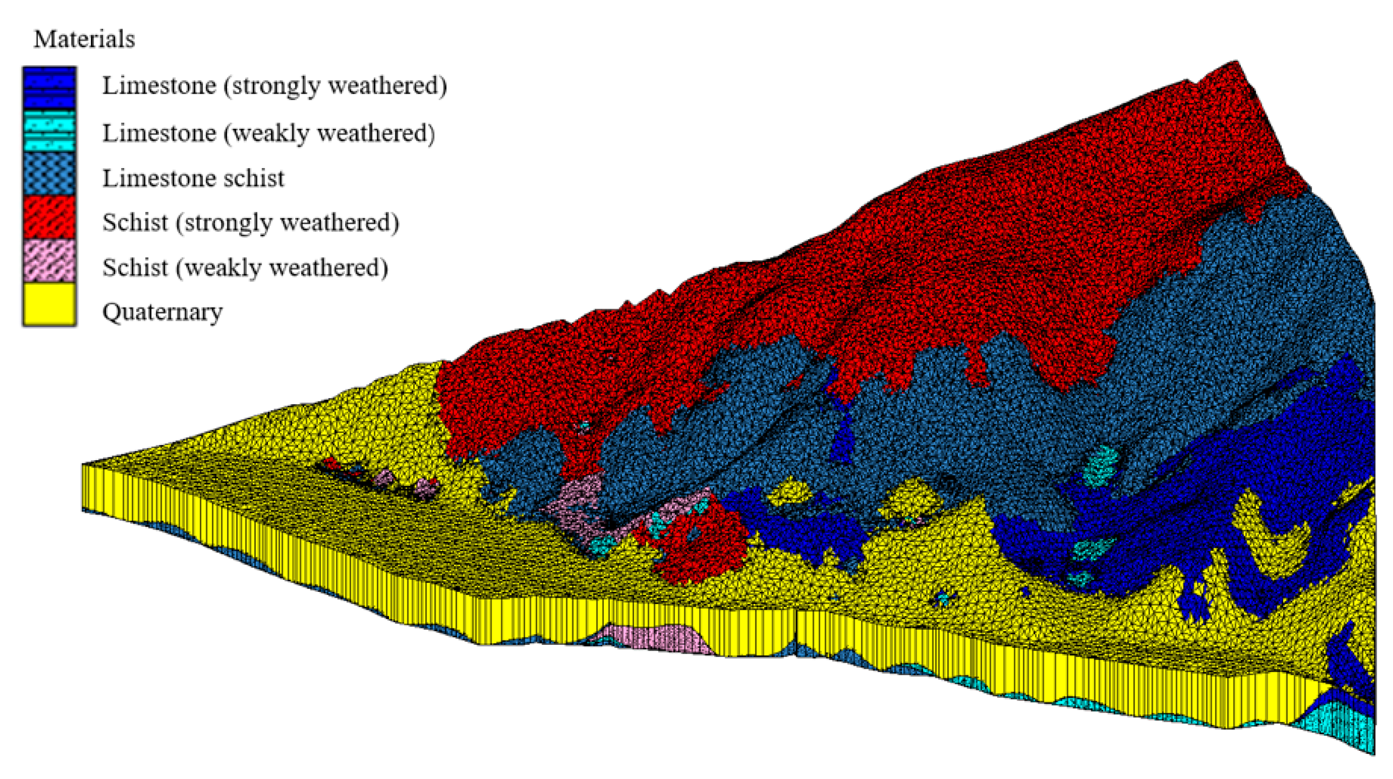
| Lithology | Kx (cm/s) | Kx/Ky | Kx/Kz |
|---|---|---|---|
| Limestone (strongly weathered) | 1.4 × 10⁻³ | 1 | 3 |
| Limestone (weakly weathered) | 6.95 × 10⁻⁴ | 1 | 3 |
| Limestone schist | 3.5 × 10⁻⁴ | 1 | 3 |
| Schist (strongly weathered) | 1.16 × 10⁻⁵ | 1 | 1 |
| Schist (weakly weathered) | 1.16 × 10⁻⁶ | 1 | 1 |
| Quaternary | 1.16 × 10⁻² | 1 | 2 |
| Engineering Parts | C (m2/d) | Elevation of Water Outlet Point (m) | Water Inflow Date | Water Inflow (m3/d) | Forecast Water Inflow (m3/d) |
|---|---|---|---|---|---|
| Main room | 5.51 | 1794.5 | 21.6–21.9 | 1440 | 1436.54 |
| Traffic room | 3.53 | 1800.4 | 21.9 | 1680 | 1005.95 |
| Outlet room | 2.26 | 1765 | 21.10–21.11 | 1200 | 1445.17 |
Disclaimer/Publisher’s Note: The statements, opinions and data contained in all publications are solely those of the individual author(s) and contributor(s) and not of MDPI and/or the editor(s). MDPI and/or the editor(s) disclaim responsibility for any injury to people or property resulting from any ideas, methods, instructions or products referred to in the content. |
© 2024 by the authors. Licensee MDPI, Basel, Switzerland. This article is an open access article distributed under the terms and conditions of the Creative Commons Attribution (CC BY) license (https://creativecommons.org/licenses/by/4.0/).
Share and Cite
Chen, Z.; Su, Z.; Li, M.; Shen, Q.; Fan, L.; Zhang, Y. Investigation of the Tunnel Water Inflow Prediction Method Based on the MODFLOW-DRAIN Module. Water 2024, 16, 1078. https://doi.org/10.3390/w16081078
Chen Z, Su Z, Li M, Shen Q, Fan L, Zhang Y. Investigation of the Tunnel Water Inflow Prediction Method Based on the MODFLOW-DRAIN Module. Water. 2024; 16(8):1078. https://doi.org/10.3390/w16081078
Chicago/Turabian StyleChen, Zhou, Zhaoqiang Su, Mei Li, Qi Shen, Lufei Fan, and Yanjie Zhang. 2024. "Investigation of the Tunnel Water Inflow Prediction Method Based on the MODFLOW-DRAIN Module" Water 16, no. 8: 1078. https://doi.org/10.3390/w16081078
APA StyleChen, Z., Su, Z., Li, M., Shen, Q., Fan, L., & Zhang, Y. (2024). Investigation of the Tunnel Water Inflow Prediction Method Based on the MODFLOW-DRAIN Module. Water, 16(8), 1078. https://doi.org/10.3390/w16081078