
Influence of Fluvial Discharges and Tides on the Salt Wedge Position of a Microtidal Estuary: Magdalena River


Abstract
:1. Introduction
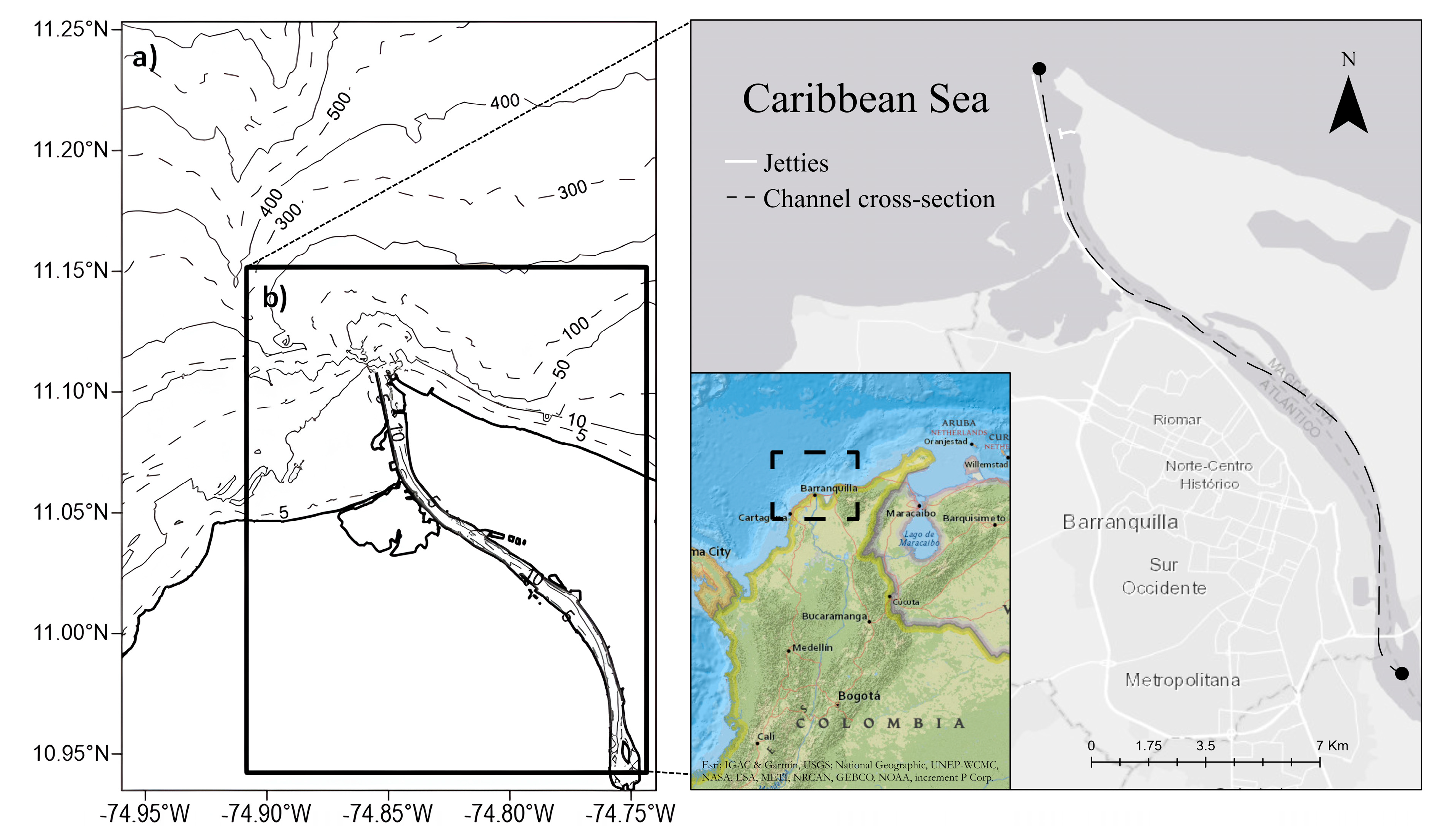
2. Study Area
3. Methodology
3.1. Stratification and Mixing Parameters
3.2. Definition of the Flow Scenarios
4. Results
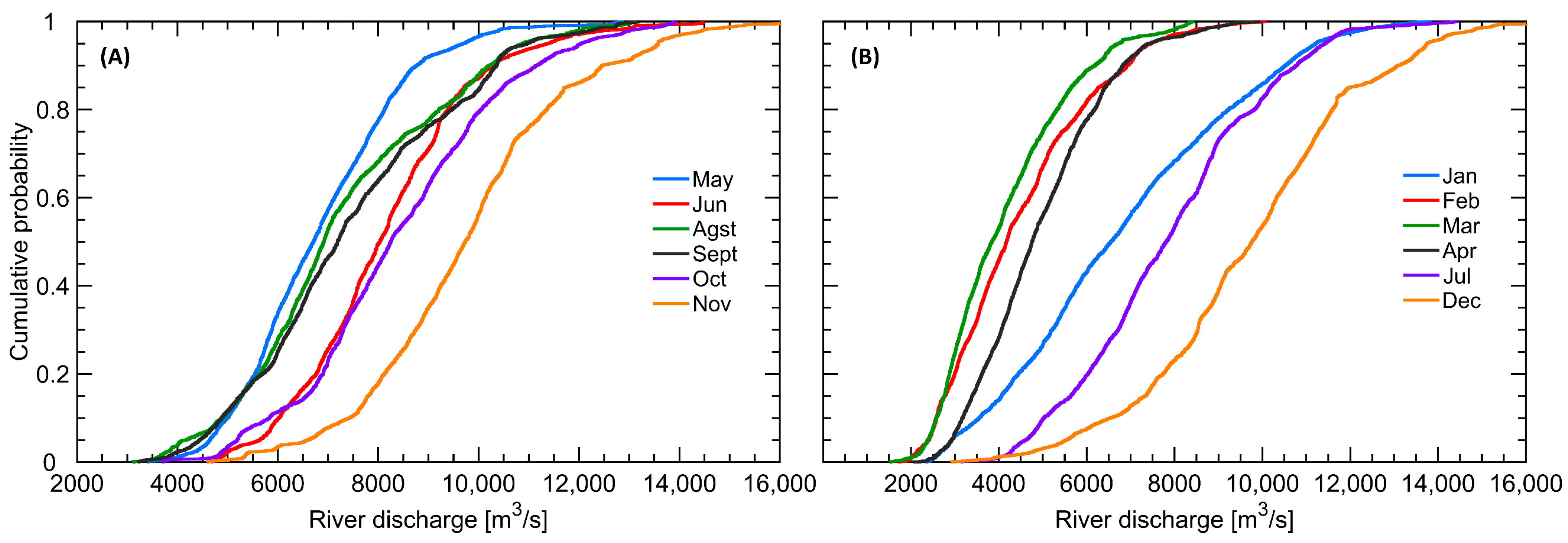
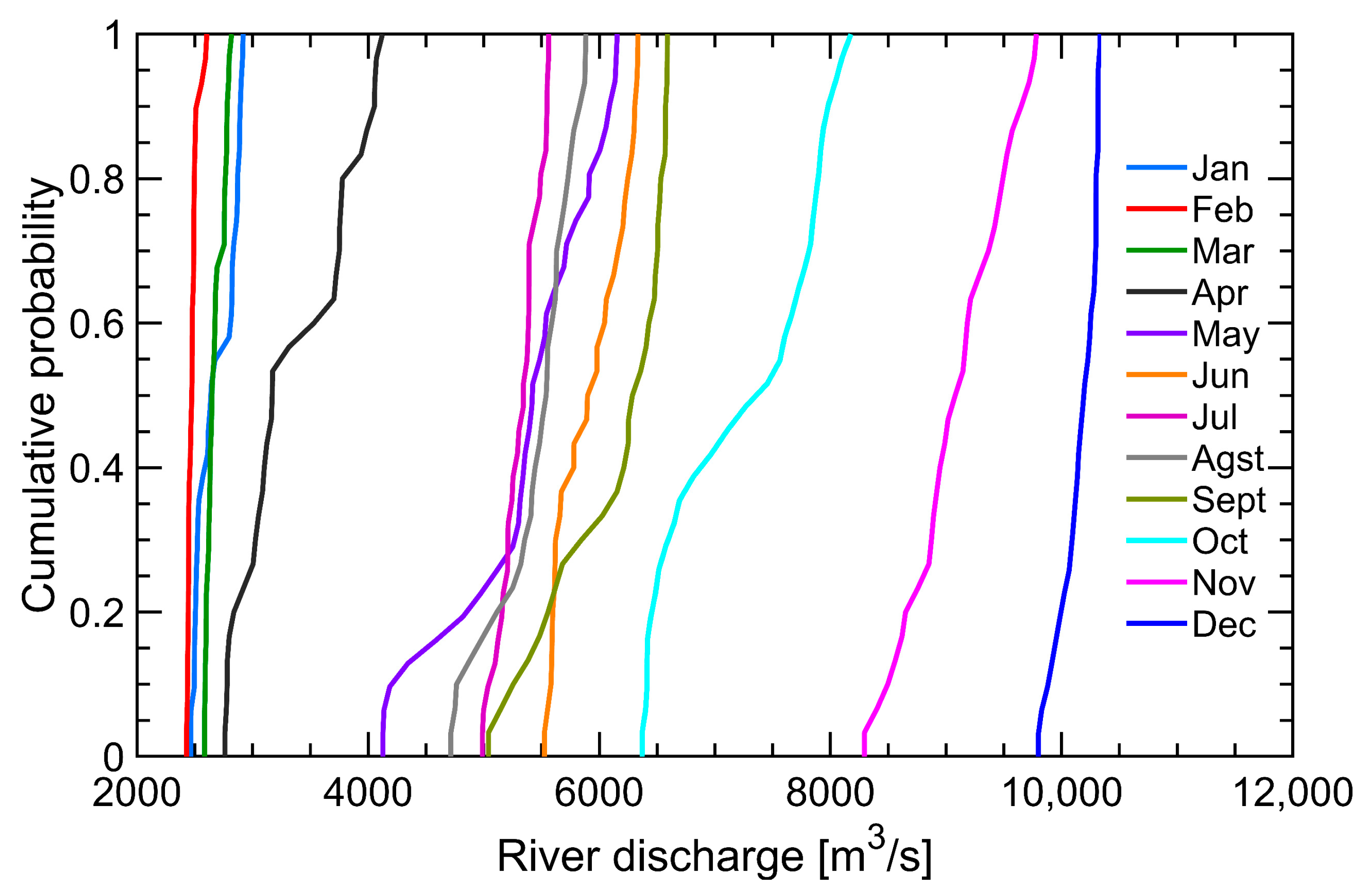
4.1. Average Monthly Flow Rate
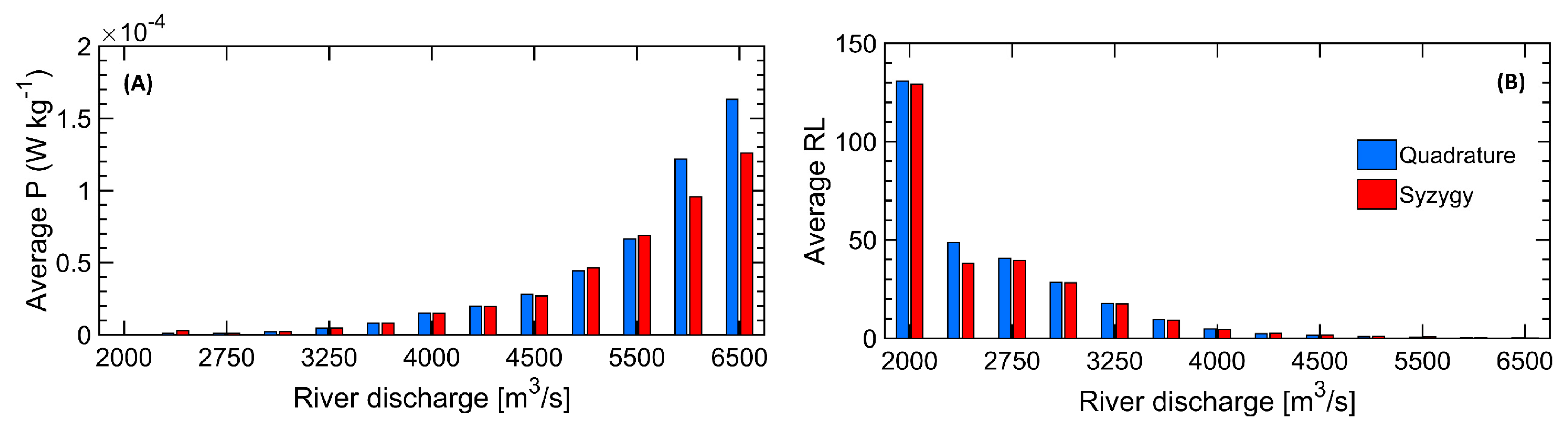
4.2. Tidal Effects on the Stratification and Penetration of the Salt Wedge
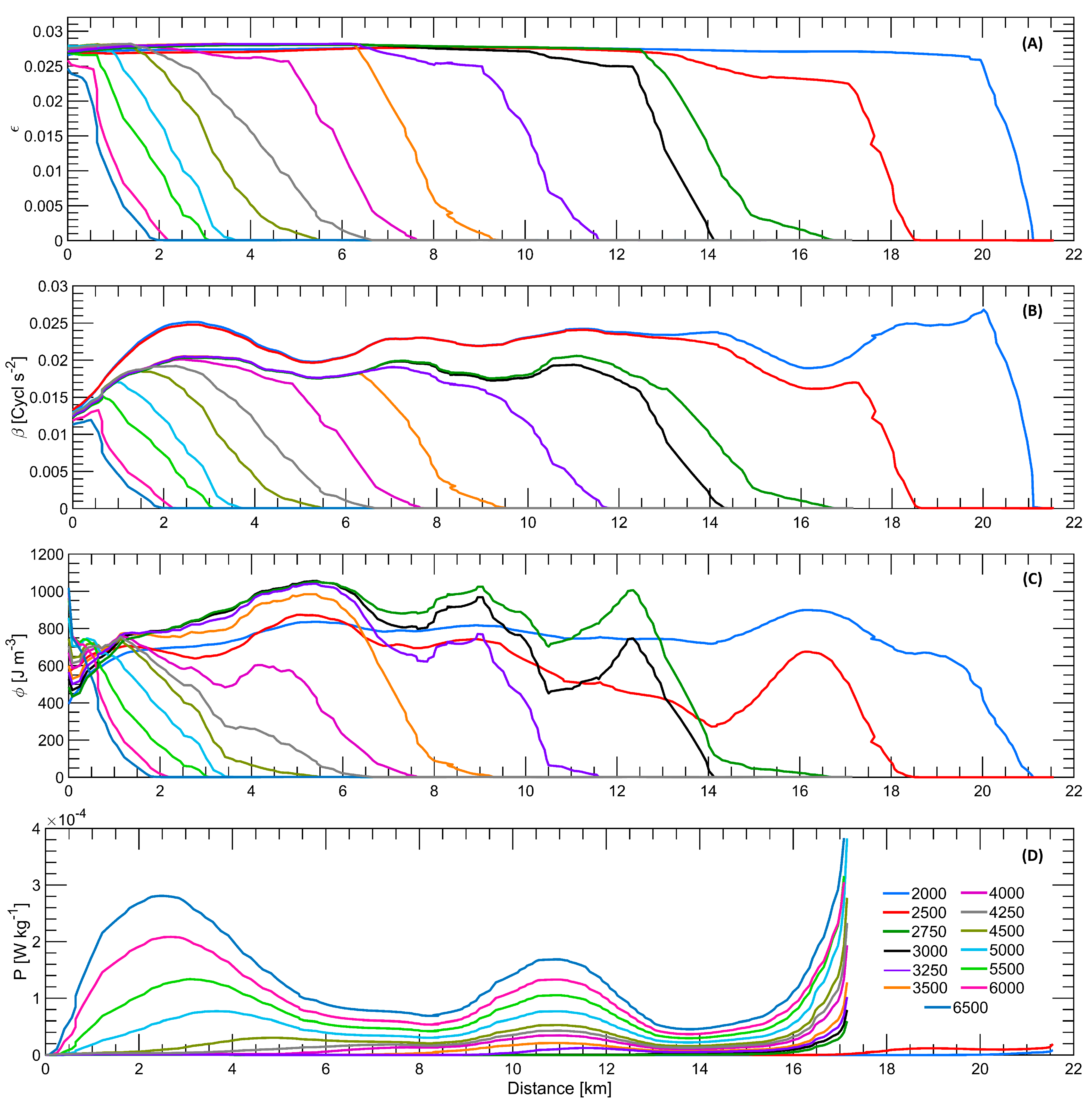
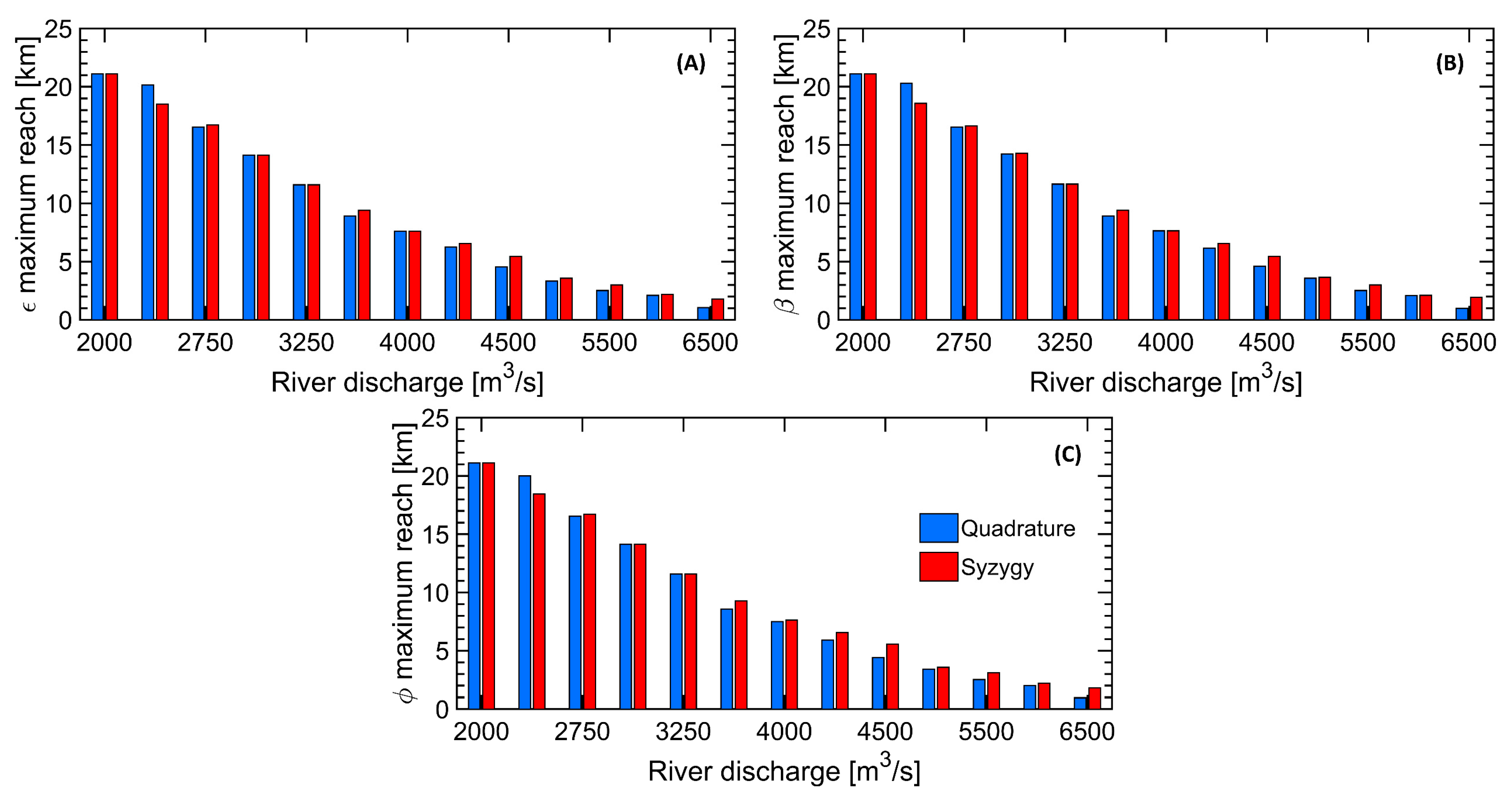
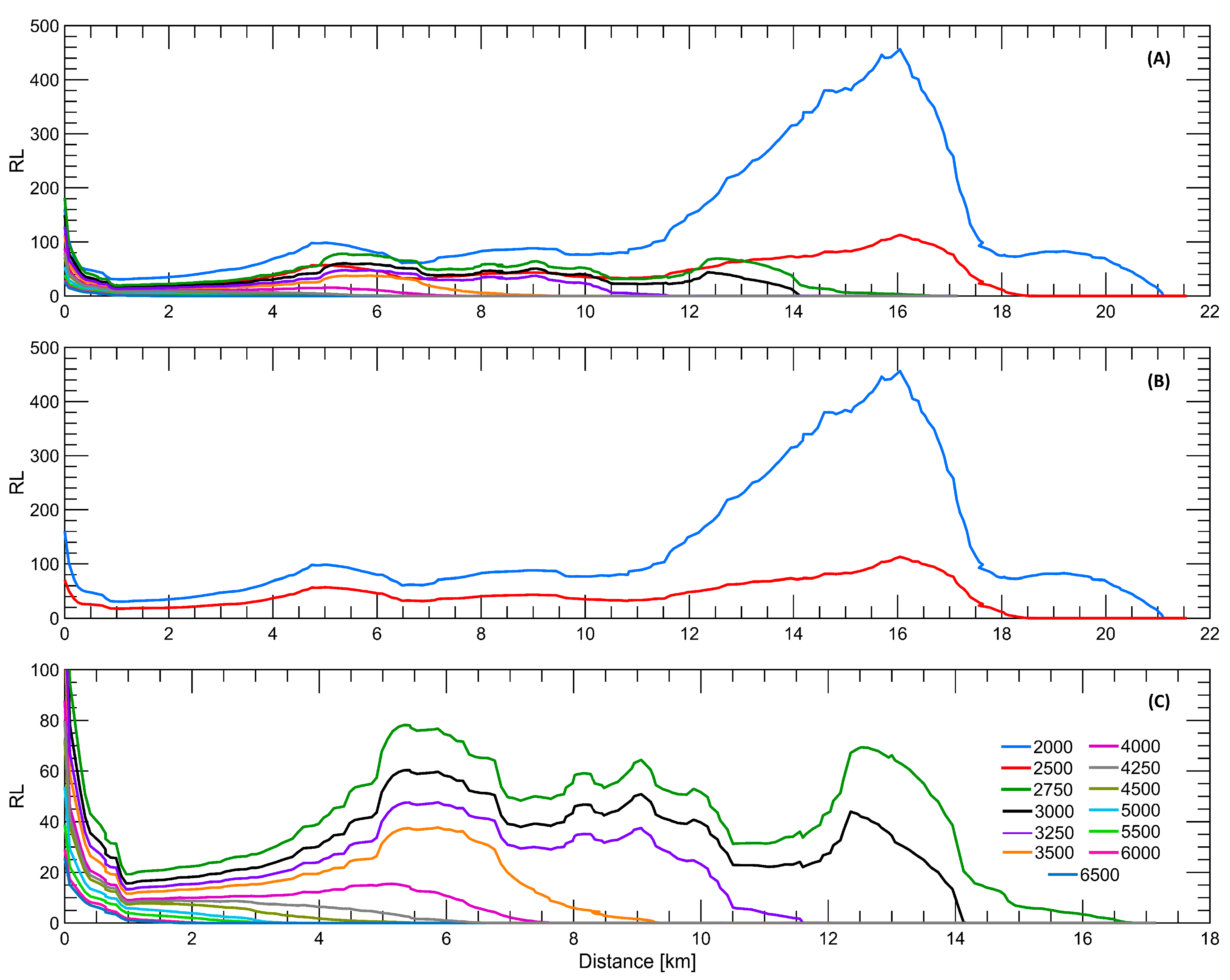
4.3. Effects of Flow Rate on FSI Position
- FSI for Flow Rates from 2000 to 3000 m3/s
- FSI for Flow Rates from 3250 to 4000 m3/s
- FSI for Flow Rates from 4250 to 6500 m3/s
5. Discussion
5.1. Tidal and Flow Effects on the Salt Wedge
5.2. FSI Monthly Mobility
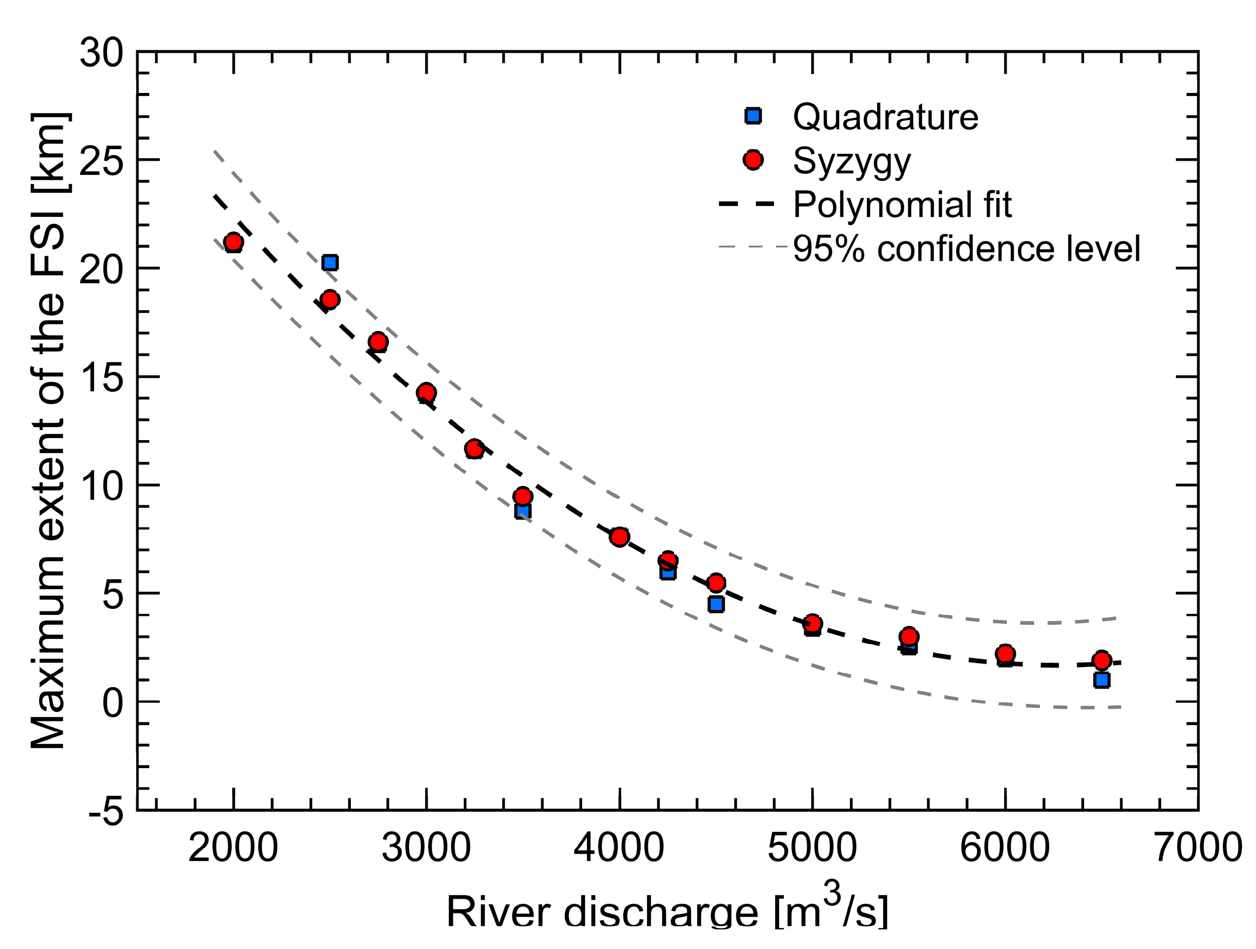
5.3. Probabilistic Model Validation
6. Conclusions
Author Contributions
Funding
Data Availability Statement
Conflicts of Interest
References
- Pritchard, D.W. Estuarine circulation patterns. Proc. Am. Soc. Civil Eng. 1955, 81, 1–11. [Google Scholar]
- Geyer, W.R.; MacCready, P. The Estuarine Circulation. Annu. Rev. Fluid. Mech. 2014, 46, 175–197. [Google Scholar] [CrossRef]
- Valle-Levinson, A. 1.05-Classification of Estuarine Circulation. In Treatise on Estuarine and Coastal Science; Wolanski, E., McLusky, D., Eds.; Elsevier: Amsterdam, The Netherlands, 2011; pp. 75–86. [Google Scholar]
- Haas, L.W. The effect of the spring-neap tidal cycle on the vertical salinity structure of the James, York and Rappahannock Rivers, Virginia, U.S.A. Estuar. Coast. Mar. Sci. 1977, 5, 485–496. [Google Scholar] [CrossRef]
- Dyer, K.R.; New, A.L. Intermittency in Estuarine Mixing. In Estuarine Variability; Wolfe, D.A., Ed.; Academic Press: Cambridge, MA, USA, 1986; pp. 321–339. [Google Scholar]
- Valle-Levinson, A. Contemporary Issues in Estuarine Physics; Valle-Levinson, A., Ed.; Cambridge University Press: Cambridge, UK, 2010. [Google Scholar]
- MacCready, P.; Geyer, W.R. Advances in estuarine physics. Annu. Rev. Mar. Sci. 2010, 2, 35–58. [Google Scholar] [CrossRef] [PubMed]
- Hansen, D.V.; Rattray, M., Jr. New Dimensions in Estuary Classification1. Limnol. Oceanogr. 1966, 11, 319–326. [Google Scholar] [CrossRef]
- Perales-Valdivia, H.; Sanay-González, R.; Valle-Levinson, A. Effects of tides, wind and river discharge on the salt intrusion in a microtidal tropical estuary. Reg. Stud. Mar. Sci. 2018, 24, 400–410. [Google Scholar] [CrossRef]
- Zachopoulos, K.; Kokkos, N.; Sylaios, G. Salt wedge intrusion modeling along the lower reaches of a Mediterranean river. Reg. Stud. Mar. Sci. 2020, 39, 101467. [Google Scholar] [CrossRef]
- Couceiro, M.A.A.; Schettini, C.A.F.; Siegle, E. Modeling an arrested salt-wedge estuary subjected to variable river flow. Reg. Stud. Mar. Sci. 2021, 47, 101993. [Google Scholar] [CrossRef]
- Krvavica, N.; Gotovac, H.; Lončar, G. Salt-wedge dynamics in microtidal Neretva River estuary. Reg. Stud. Mar. Sci. 2021, 43, 101713. [Google Scholar] [CrossRef]
- Paiva, B.P.; Schettini, C.A.F. Circulation and transport processes in a tidally forced salt-wedge estuary: The São Francisco river estuary, Northeast Brazil. Reg. Stud. Mar. Sci. 2021, 41, 101602. [Google Scholar] [CrossRef]
- Uncles, R.; Ong, J.; Gong, W. Observations and analysis of a stratification destratification event in a tropical estuary. Estuar. Coast Shelf Sci. 1990, 31, 651–665. [Google Scholar] [CrossRef]
- Newton, A.; Icely, J.; Cristina, S.; Brito, A.; Cardoso, A.C.; Colijn, F.; Riva, S.D.; Gertz, F.; Hansen, J.W.; Holmer, M.; et al. An overview of ecological status, vulnerability and future perspectives of European large shallow, semi-enclosed coastal systems, lagoons and transitional waters. Estuar. Coast. Shelf Sci. 2014, 140, 95–122. [Google Scholar] [CrossRef]
- Huang, P.; Kilminster, K.; Larsen, S.; Hipsey, M.R. Assessing artificial oxygenation in a riverine salt-wedge estuary with a three-dimensional finite-volume model. Ecol. Eng. 2018, 118, 111–125. [Google Scholar] [CrossRef]
- Dyer, K. Estuarine Circulation. In Encyclopedia of Ocean Sciences; Steele, J.H., Ed.; Elsevier: Amsterdam, The Netherlands, 2001; pp. 846–852. [Google Scholar]
- Guo, L.; He, Q. Freshwater flocculation of suspended sediments in the Yangtze River, China. Ocean Dyn. 2011, 61, 371–386. [Google Scholar] [CrossRef]
- Silva-Dias, F.J.; Castro, B.M.; Lacerda, L.D.; Miranda, L.B.; Marins, R.V. Physical characteristics and discharges of suspended particulate matter at the continent-ocean interface in an estuary located in a semiarid region in northeastern Brazil. Estuar. Coast. Shelf Sci. 2016, 180, 258–274. [Google Scholar] [CrossRef]
- Restrepo, J.C.; Orejarena-Rondón, A.; Consuegra, C.; Pérez, J.; Llinas, H.; Otero, L.; Álvarez, O. Siltation on a highly regulated estuarine system: The Magdalena River mouth case (Northwestern South America). Estuar. Coast. Shelf Sci. 2020, 245, 107020. [Google Scholar] [CrossRef]
- Ming, Y.; Gao, L. Flocculation of suspended particles during estuarine mixing in the Changjiang estuary-East China Sea. J. Mar. Syst. 2022, 233, 103766. [Google Scholar] [CrossRef]
- Geyer, W.R.; Woodruff, J.D.; Traykovski, P. Sediment Transport and Trapping in the Hudson River Estuary. Estuaries 2001, 24, 670–679. [Google Scholar] [CrossRef]
- Li, M.; Ge, J.; Kappenberg, J.; Much, D.; Nino, O.; Chen, Z. Morphodynamic processes of the Elbe River estuary, Germany: The Coriolis effect, tidal asymmetry and human dredging. Front. Earth Sci. 2013, 8, 181–189. [Google Scholar] [CrossRef]
- Orseau, S.; Huybrechts, N.; Tassi, P.; Van Bang, D.P.; Klein, F. Two-dimensional modeling of fine sediment transport with mixed sediment and consolidation: Application to the Gironde Estuary, France. Int. J. Sediment Res. 2021, 36, 736–746. [Google Scholar] [CrossRef]
- Urbano Latorre, C.P.; Otero Díaz, L.J.; Lonin, S. Influencia de las corrientes en los campos de oleaje en el área de Bocas de Ceniza, Caribe Colombiano. Boletín Científico CIOH 2013, 31, 191–206. [Google Scholar] [CrossRef]
- Assessment LC. 2.1.2 Colombia Port of Barranquilla [Internet]. 2021. Available online: https://dlca.logcluster.org/212-colombia-port-barranquilla (accessed on 18 December 2023).
- MIN.TRANSPORTE. Cormagdalena y Findeter garantizan dragado en el río Magdalena en el 2021 gracias a la suscripción del contrato interadministrativo. Sitio web nacional Ministerio de Transporte Publicación [Internet]. 2020. Available online: https://mintransporte.gov.co/publicaciones/9296/cormagdalena-y-findeter-garantizan-dragado-en-el-rio-magdalena-en-el-2021-gracias-a-la-suscripcion-del-contrato-interadministrativo/ (accessed on 18 December 2023).
- Jang, D.; Hwang, J.H.; Park, Y.-G.; Park, S.-H. A study on salt wedge and River Plume in the Seom-Jin River and estuary. KSCE J. Civ. Eng. 2012, 16, 676–688. [Google Scholar] [CrossRef]
- Ospino, S.; Restrepo, J.C.; Otero, L.; Pierini, J.; Alvarez-Silva, O. Saltwater intrusion into a river with high fluvial discharge: A microtidal estuary of the Magdalena River, Colombia. J. Coast Res. 2018, 34, 1273–1288. [Google Scholar]
- Álvarez, A.H.; Otero, L.; Restrepo, J.C.; Álvarez, O. The effect of waves in hydrodynamics, stratification, and salt wedge intrusion in a microtidal estuary. Front. Mar. Sci. 2022, 9, 2296–7745. [Google Scholar]
- Restrepo, J.C.; Schrottke, K.; Traini, C.; Bartholomae, A.; Ospino, S.; Ortíz, J.C.; Otero, L.; Orejarena, A. Estuarine and sediment dynamics in a microtidal tropical estuary of high fluvial discharge: Magdalena River (Colombia, South America). Mar. Geol. 2018, 398, 86–98. [Google Scholar] [CrossRef]
- Arevalo, F.M.; Álvarez-Silva, Ó.; Caceres-Euse, A.; Cardona, Y. Mixing mechanisms at the strongly-stratified Magdalena River’s estuary and plume. Estuar. Coast. Shelf Sci. 2022, 277, 108077. [Google Scholar] [CrossRef]
- Restrepo, J.C.; Ospino, O.; Torregroza-Espinosa, A.C.; Ospino, S.; Villanueva, E.; Molano-Mendoza, J.C.; Consuegra, C.; Agrawal, Y.; Mikkelsen, O. Variability of suspended sediment properties in the saline front of the highly stratified Magdalena River estuary, Colombia. J. Mar. Syst. 2024, 241, 103894. [Google Scholar] [CrossRef]
- Otero, L.J.; Hernandez, H.I.; Higgins, A.E.; Restrepo, J.C.; Álvarez, O.A. Interannual and seasonal variability of stratification and mixing in a high-discharge micro-tidal delta: Magdalena River, Colombia. J. Mar. Syst. 2021, 224, 103621. [Google Scholar] [CrossRef]
- Álvarez, O.; Osorio, A. Salinity gradient energy potential in Colombia considering site specific constraints, Colombia. Renew. Energy 2015, 74, 737–748. [Google Scholar] [CrossRef]
- Roldan-Carvajal, M.; Vallejo-Castaño, S.; Álvarez-Silva, O.; Bernal-García, S.; Arango-Aramburo, S.; Sánchez-Sáenz, C.I.; Osorio, A.F. Salinity gradient power by reverse electrodialysis: A multidisciplinary assessment in the Colombian context. Desalination 2021, 503, 114933. [Google Scholar] [CrossRef]
- Sheppard, C. The Estuarine Ecosystem: Ecology, Threats and Management, Third Edition. Mar. Pollut. Bull. 2004, 49, 9–10. [Google Scholar] [CrossRef]
- Statham, P.J. Nutrients in estuaries—An overview and the potential impacts of climate change. Sci. Total Environ. 2012, 434, 213–227. [Google Scholar] [CrossRef] [PubMed]
- Torregroza, A.C. Spatio-temporal distribution of temperature, salinity, and suspended sediment on the deltaic front of the Magdalena River: Influence on nutrient concentration and primary productivity. J. Artic. Salin. Mar. Sediments 2020, 24, 10–120. [Google Scholar]
- Higgins, A.; Restrepo, J.C.; Ortíz, J.; Pierini, J.; Otero, L. Suspended Sediment Transport in the Magdalena River (Colombia, South America): Hydrologic Regime, Rating Parameters and Effective Discharge Variability. Int. J. Sediment Res. 2015, 31, 25–35. [Google Scholar] [CrossRef]
- Restrepo, J.C.; Ortíz, J.; Otero, L.; Ospino, S. Transporte de sedimentos en suspensión en los principales ríos del Caribe colombiano: Magnitud, tendencias y variabilidad. Rev. Acad. Colomb. Cienc. Exactas Fis. Nat. 2015, 39, 527–546. [Google Scholar] [CrossRef]
- Milliman, J.; Farnsworth, K. River Discharge to the Coastal Ocean: A Global Synthesis; Cambridge University Press: Cambridge, UK, 2011. [Google Scholar]
- Restrepo, J.C.; Schrottke, K.; Traini, C.; Ortíz, J.C.; Orejarena, A.; Otero, L.; Higgins, A.; Marriaga, L. Sediment Transport Regime and Geomorphological Change in a High Discharge Tropical Delta (Magdalena River, Colombia): Insights from a Period of Intense Change and Human Intervention (1990–2010). J. Coast. Res. 2015, 32, 575–589. [Google Scholar]
- Pérez-Santos, I.; Schneider, W.; Sobarzo, M.; Montoya-Sánchez, R.; Valle-Levinson, A.; Garcés-Vargas, J. Surface wind variability and its implications for the Yucatan basin-Caribbean Sea dynamics. J. Geophys. Res. Atmos. 2010, 115, 10052. [Google Scholar] [CrossRef]
- Ruiz, O.M. Variabilidad de la Cuenca Colombia (mar Caribe) Asociada con El Niño-Oscilación del Sur, Vientos Alisios y Procesos Locales. Deoartamento de Geociencias y Medio Ambiente, UNAL [Internet]. 2011. Available online: https://repositorio.unal.edu.co/handle/unal/8181 (accessed on 18 December 2023).
- Ortiz, J.; Otero, L.; Restrepo, J.C.; Ruiz, J.; Cadena, M. Characterization of cold fronts in the Colombian Caribbean and their relationship to extreme wave events. Nat. Hazards Earth Syst. Sci. 2013, 13, 2797–2804. [Google Scholar] [CrossRef]
- Torregroza-Espinosa, A.C.; Restrepo, J.C.; Escobar, J.; Pierini, J.; Newton, A. Spatial and temporal variability of temperature, salinity and chlorophyll-a in the Magdalena River mouth, Caribbean Sea. J. S. Am. Earth Sci. 2021, 105, 102978. [Google Scholar] [CrossRef]
- Tejeda-Benitez, L.; Flegal, R.; Odigie, K.; Olivero-Verbel, J. Pollution by metals and toxicity assessment using Caenorhabditis elegans in sediments from the Magdalena River, Colombia. Environ. Pollut. 2016, 212, 238–250. [Google Scholar] [CrossRef]
- Tejeda-Benítez, L.; Noguera-Oviedo, K.; Aga, D.S.; Olivero-Verbel, J. Toxicity profile of organic extracts from Magdalena River sediments. Environ. Sci. Pollut. Res. 2018, 25, 1519–1532. [Google Scholar] [CrossRef] [PubMed]
- Molares, B.R. Clasificación e identificación de las componentes de marea del Caribe colombiano. Boletín Científico CIOH 2004, 24, 105–114. [Google Scholar] [CrossRef]
- Restrepo, J.D.; López, S.A. Morphodynamics of the Pacific and Caribbean deltas of Colombia, South America. J. S. Am. Earth Sci. 2008, 25, 1–21. [Google Scholar] [CrossRef]
- Pérez, R.A.; Ortiz, R.J.C.; Bejarano, A.L.F.; Otero, D.L.; Restrepo, L.J.C.; Franco, H.A. Sea breeze in the Colombian Caribbean coast. Atmósfera 2018, 31, 389–406. [Google Scholar] [CrossRef]
- Bedoya-Soto, J.M.; Poveda, G.; Trenberth, K.E.; Vélez-Upegui, J.J. Interannual hydroclimatic variability and the 2009–2011 extreme ENSO phases in Colombia: From Andean glaciers to Caribbean lowlands. Theor. Appl. Clim. 2019, 135, 1531–1544. [Google Scholar] [CrossRef]
- Cai, W.; McPhaden, M.; Grimm, A.; Rodrigues, R.; Taschetto, A.; Garreaud, R. Climate impacts of the El Niño–Southern Oscillation on South America. Nat. Rev. Earth Environ. 2020, 1, 215–231. [Google Scholar] [CrossRef]
- Vega, M.J.; Alvarez-Silva, O.; Restrepo, J.C.; Ortiz, J.C.; Otero, L.J. Interannual variability of wave climate in the Caribbean Sea. Ocean Dyn. 2020, 70, 965–976. [Google Scholar] [CrossRef]
- Higgins, A.; Otero, L.; Restrepo, J.C.; Álvarez, O. Variabilidad estacional de la interacción oleaje-corriente y dinámica de la cuña salina en la desembocadura del Delta del río Magdalena. In Libro de Resúmenes Extendidos XVI Senalmar; INVEMAR-ACIMAR, Colombia, Ed.; 2017; pp. 76–80. [Google Scholar]
- Higgins, A.; Restrepo, J.C.; Otero, L.; Ortiz, J.C.; Conde, M. Vertical distribution of suspended sediment in the mouth area of the Magdalena River, Colombia. Lat. Am. J. Aquat. Res. 2017, 45, 724–736. [Google Scholar] [CrossRef]
- Maretec. Mohid Water [Internet]. Mohid Official Webpage. 2020. Available online: http://www.mohid.com/pages/models/mohidwater/mohid_water_home.shtml (accessed on 18 December 2023).
- Martins, F.; Neves, R.; Leitao, P.; Silva, A. 3D modeling in the Sado estuary using a new generic vertical discretization approach. Oceanol. Acta 2001, 24, 51–62. [Google Scholar] [CrossRef]
- Arakawa, A. Computational design for long-term numerical integration of the equations of fluid motion: Two-dimensional incompressible flow. Part I. J. Comput. Phys. 1966, 1, 119–143. [Google Scholar] [CrossRef]
- Leendertse, J.J. Aspects of a Computational Model for Long-Period Water-Wave Propagation; RAND Corporation: Santa Monica, CA, USA, 1967. [Google Scholar]
- Abbott, M.B.; Damsgaard, A.; Rodenhuis, G.S. System 21, Jupiter, a design system for two-dimensional nearly horizontal flows. J. Hydraul. Res. 1973, 11, 1–28. [Google Scholar] [CrossRef]
- Canuto, V.M.; Howard, A.; Cheng, Y.; Dubovikov, M.S. Ocean turbulence I: One-point closure model—Momentum and heat vertical diffusivities. J. Phys. Oceanogr. 2001, 31, 1413–1426. [Google Scholar] [CrossRef]
- Willmott, C.J.; Ackleson, S.G.; Davis, R.E.; Feddema, J.J.; Klink, K.M.; Legates, D.R.; O’Donnell, J.; Rowe, C.M. Statistics for the evaluation and comparison of models. J. Geophys Res. Oceans 1985, 90, 8995–9005. [Google Scholar] [CrossRef]
- Geyer, W.R.; Scully, M.E.; Ralston, D.K. Quantifying vertical mixing in estuaries. Environ. Fluid Mech. 2008, 8, 495–509. [Google Scholar] [CrossRef]
- Simpson, J.; Crisp, D.; Hearn, C. The shelf-sea fronts: Implications of their existence and behaviour and discussion. Philos. Trans. R. Soc. London. Ser. A Math. Phys. Sci. 1981, 302, 531–546. [Google Scholar]
- MacKay, H.; Schumann, E. Mixing and circulation in the Sundays River estuary, South Africa. Estuar. Coast Shelf Sci. 1990, 31, 203–216. [Google Scholar] [CrossRef]
- Ralston, D.K.; Geyer, W.R.; Lerczak, J.A.; Scully, M. Turbulent mixing in a strongly forced salt wedge estuary. J. Geophys. Res. Oceans 2010, 115, 12024. [Google Scholar] [CrossRef]
- IDEAM. Serie de Caudal Medio Diario. Periodo 23/07/1940 y 31/12/2015. Estación Limnimétrica CALAMAR [29037020]. Departamento de Bolívar, Municipio Calamar [Internet]. Available online: http://dhime.ideam.gov.co/atencionciudadano/ (accessed on 18 December 2023).
- Pernot, P.; Savin, A. Probabilistic performance estimators for computational chemistry methods: The empirical cumulative distribution function of absolute errors. J. Chem. Phys. 2018, 148, 241707. [Google Scholar] [CrossRef]
- Wischik, D. Foundations of Data Science [Internet]. University of Cambridge. 2020. Available online: https://www.youtube.com/watch?v=JrS1ajLqMZQ&list=PLknxdt7zG11O5BV8ipHD30dnupEk-tKjn&index=24 (accessed on 18 December 2023).
- Thorn, M. Coastal and estuarine sediment dynamics by K.R. Dyer. Wiley, Chichester, 1986. No. of pages: 358. Geol. J. 1987, 22, 169. Available online: https://onlinelibrary.wiley.com/doi/abs/10.1002/gj.3350220210 (accessed on 18 December 2023). [CrossRef]
- Pritchard, D.W. Estuarine Classification—A Help or a Hindrance. In Estuarine Circulation; Neilson Bruce, J., Kuo, A.B.J., Eds.; Humana Press: Totowa, NJ, USA, 1989; pp. 1–38. [Google Scholar] [CrossRef]
- Holford, J.M.; Linden, P.F. Turbulent Mixing in a Stratified Fluid. Dyn. Atmos. Ocean. 1999, 30, 173–198. Available online: https://www.sciencedirect.com/science/article/pii/S0377026599000251 (accessed on 18 December 2023). [CrossRef]
- Read, J.S.; Hamilton, D.P.; Jones, I.D.; Muraoka, K.; Winslow, L.A.; Kroiss, R.; Wu, C.H.; Gaiser, E. Derivation of lake mixing and stratification indices from high-resolution lake buoy data. Environ. Model. Softw. 2011, 26, 1325–1336. [Google Scholar] [CrossRef]
- Burchard, H.; Hofmeister, R. A dynamic equation for the potential energy anomaly for analysing mixing and stratification in estuaries and coastal seas. Estuar. Coast. Shelf Sci. 2008, 77, 679–687. Available online: https://www.sciencedirect.com/science/article/pii/S0272771407004945 (accessed on 18 December 2023). [CrossRef]
- Hamada, T.; Kim, S. Stratification potential-energy anomaly index standardized by external tide level. Estuar. Coast. Shelf Sci. 2020, 250, 107138. Available online: https://www.sciencedirect.com/science/article/pii/S0272771420308696 (accessed on 18 December 2023). [CrossRef]
- Zhang, Z.; Cui, B.; Zhao, H.; Fan, X.; Zhang, H. Discharge-salinity relationships in Modaomen waterway, Pearl River estuary. Procedia Environ. Sci. 2010, 2, 1235–1245. Available online: https://www.sciencedirect.com/science/article/pii/S1878029610001672 (accessed on 18 December 2023). [CrossRef]
- Gisen, J.I.A.; Savenije, H.H.G.; Nijzink, R.C. Revised predictive equations for salt intrusion modelling in estuaries. Hydrol. Earth Syst. Sci. 2015, 19, 2791–2803. [Google Scholar] [CrossRef]
- Gong, W.; Shen, J. The response of salt intrusion to changes in river discharge and tidal mixing during the dry season in the Modaomen Estuary, China. Cont. Shelf Res. 2011, 31, 769–788. [Google Scholar] [CrossRef]
- Liu, W.C.; Chen, W.B.; Cheng, R.T.; Hsu, M.H.; Kuo, A.Y. Modeling the influence of river discharge on salt intrusion and residual circulation in Danshuei River estuary, Taiwan. Cont. Shelf Res. 2007, 27, 900–921. [Google Scholar] [CrossRef]
- Sirviente, S.; Sánchez-Rodríguez, J.; Gomiz-Pascual, J.J.; Bolado-Penagos, M.; Sierra, A.; Ortega, T.; Álvarez, O.; Forja, J.; Bruno, M. A numerical simulation study of the hydrodynamic effects caused by morphological changes in the Guadalquivir River Estuary. Sci. Total Environ. 2023, 902, 166084. [Google Scholar] [CrossRef]
- de Jonge, V.N.; Schuttelaars, H.M.; van Beusekom, J.E.; Talke, S.A.; de Swart, H.E. The influence of channel deepening on estuarine turbidity levels and dynamics, as exemplified by the Ems estuary. Estuar. Coast. Shelf Sci. 2014, 139, 46–59. Available online: https://www.sciencedirect.com/science/article/pii/S0272771413005544 (accessed on 18 December 2023). [CrossRef]
- Li, X.; Cai, Y.; Liu, Z.; Mo, X.; Zhang, L.; Zhang, C.; Cui, B.; Ren, Z. Impacts of river discharge, coastal geomorphology, and regional sea level rise on tidal dynamics in Pearl River Estuary. Front. Mar. Sci. 2023, 10, 1065100. [Google Scholar] [CrossRef]
- Torres, R.R.; Tsimplis, M.N. Sea-level trends and interannual variability in the Caribbean Sea. J. Geophys. Res. Oceans 2013, 118, 2934–2947. [Google Scholar] [CrossRef]
- Krvavica, N.; Ružić, I. Assessment of Sea-Level Rise Impacts on Salt-Wedge Intrusion in Idealized and Neretva River Estuary. arXiv 2020, arXiv:2001.04765. [Google Scholar] [CrossRef]
- Leung, A.T.Y.; Stronach, J.; Matthieu, J. Modelling behaviour of the saltwedge in the fraser river and its relationship with climate and man-made changes. J. Mar. Sci. Eng. 2018, 6, 130. [Google Scholar] [CrossRef]
- Burchard, H.; Baumert, H. The Formation of Estuarine Turbidity Maxima Due to Density Effects in the Salt Wedge. A Hydrodynamic Process Study. J. Phys. Oceanogr. 1998, 28, 309–321. Available online: https://journals.ametsoc.org/view/journals/phoc/28/2/1520-0485_1998_028_0309_tfoetm_2.0.co_2.xml (accessed on 18 December 2023). [CrossRef]
- Kappenberg, J.; Grabemann, I. Variability of the Mixing Zones and Estuarine Turbidity Maxima in the Elbe and Weser Estuaries. Estuaries 2001, 24, 699–706. [Google Scholar] [CrossRef]
- Ralston, D.K.; Geyer, W.R.; Warner, J.C. Bathymetric controls on sediment transport in the Hudson River estuary: Lateral asymmetry and frontal trapping. J. Geophys. Res. Oceans 2012, 117, 1–21. [Google Scholar] [CrossRef]
- Jay, D.A.; Orton, P.M.; Chisholm, T.; Wilson, D.J.; Fain, A.M.V. Particle trapping in stratified estuaries: Consequences of mass conservation. Estuaries Coasts 2007, 30, 1095–1105. [Google Scholar] [CrossRef]
- Gregory, J.; O’Melia, C.R. Fundamentals of flocculation. Crit. Rev. Environ. Control 1989, 19, 185–230. [Google Scholar] [CrossRef]
- Sholkovitz, E. Flocculation of dissolved organic and inorganic matter during the mixing of river water and seawater. Geochim. Cosmochim. Acta 1976, 40, 831–845. [Google Scholar] [CrossRef]
- Eisma, D. Flocculation and de-flocculation of suspended matter in estuaries. Neth. J. Sea Res. 1986, 20, 183–199. [Google Scholar] [CrossRef]
- Deng, Z.; He, Q.; Manning, A.J.; Chassagne, C. A laboratory study on the behavior of estuarine sediment flocculation as function of salinity, EPS and living algae. Mar. Geol. 2023, 459, 107029. [Google Scholar] [CrossRef]


| Feature | Bias | RMSE | Willmott | Source |
|---|---|---|---|---|
| Salinity | 0.04 gr/kg | 0.52 gr/kg | 0.95 | |
| Velocity | 0.0085 m/s | 0.0034 m/s | 0.7568 | [30] |
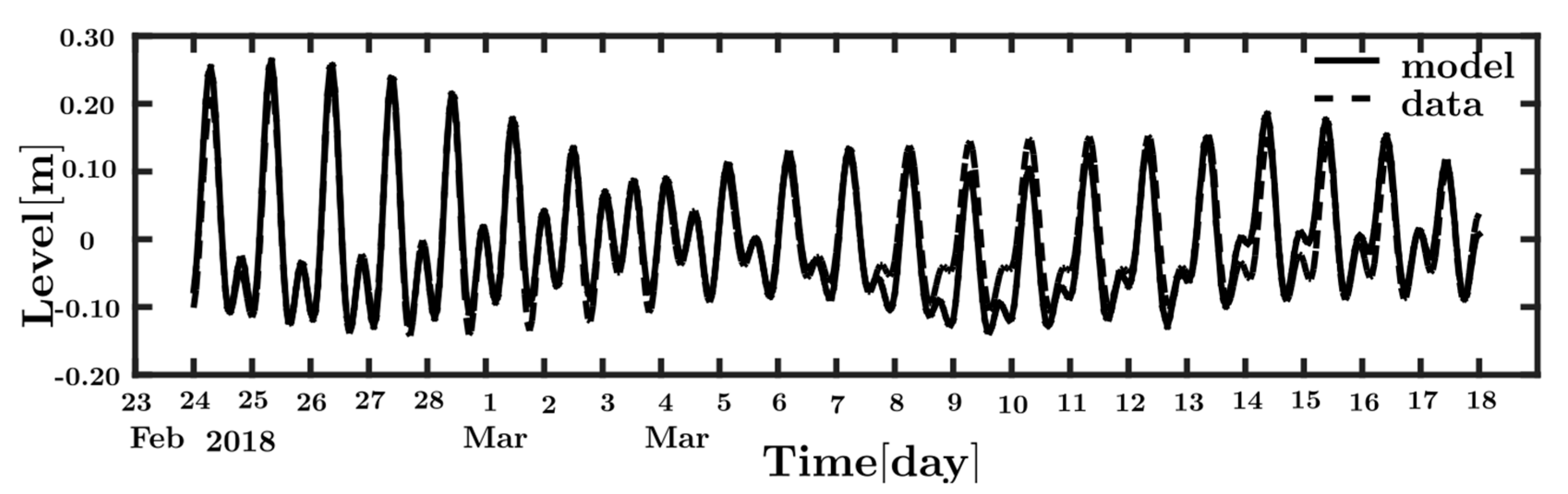
| Water level | <0.01 m | <0.01 m | 0.91–0.96 | |
| Potential energy anomaly | −0.05 | 6.2 | 0.99 | |
| Buoyancy frequency | −0.0477 | 0.00014 | 0.99 | [34] |
| Richardson number | −0.08 | 0.13 | 0.99 |
| Parameter Formulation | Meaning |
|---|---|
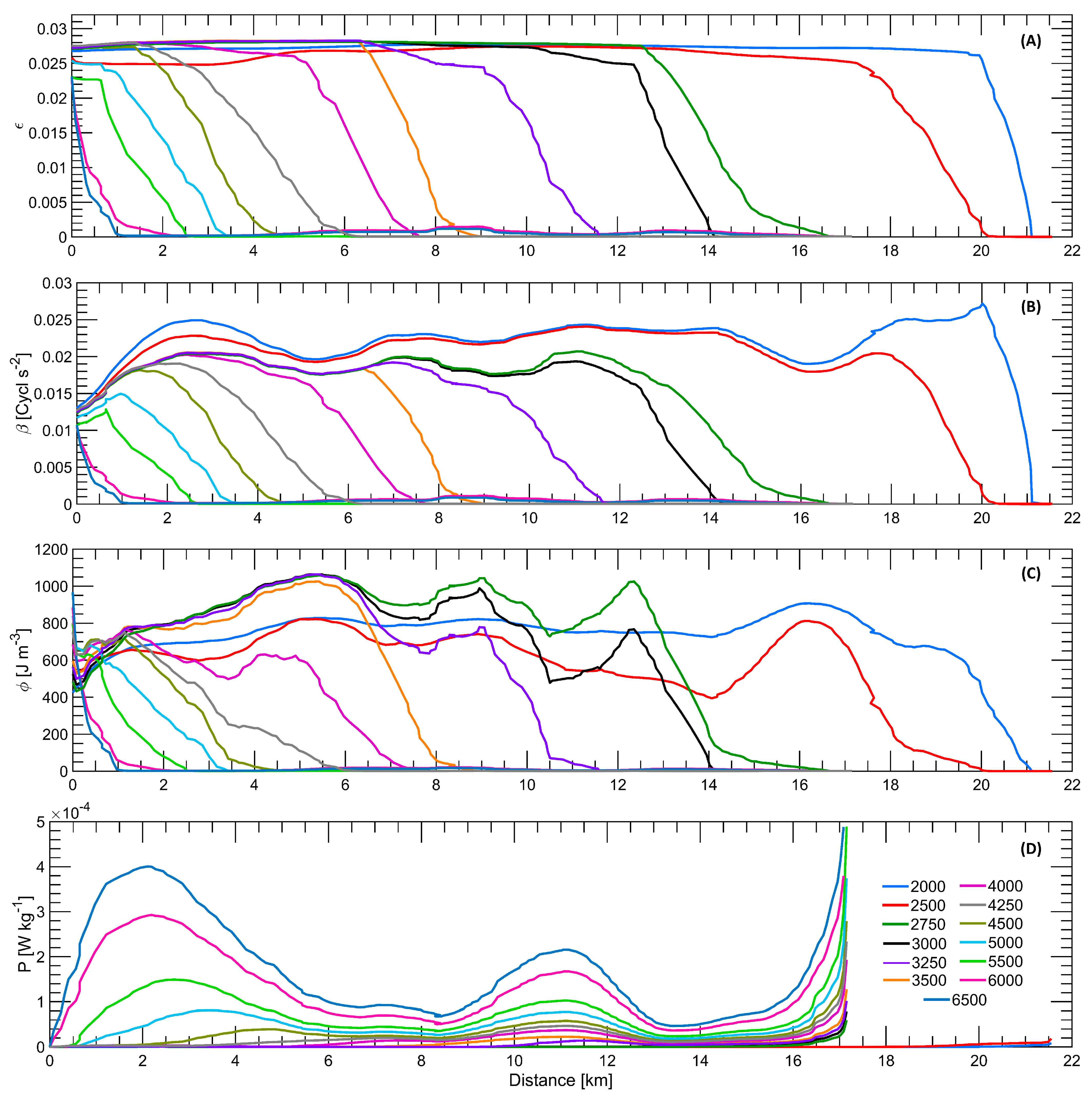
| Stratification | It is a dimensionless measurement of the stratification intensity based on the density of the water column. Here, the density gradient is represented by ∂ρ = ρ(bottom) − ρ(surface) and the average density is expressed as ρo = 0.5 (ρb + ρs). Usually, this parameter reaches values between 0 (indicating a well-mixed water plot) and 0.025 (indicating a highly stratified water plot) [8]. |
| Buoyancy Frequency | It is a cycle/s2 index of the oscillation frequency of a vertically displaced water plot (β > 0) while tending to balance hydrostatically. Here, g represents the gravity acceleration, ∂z = z(bottom) − z(surface) is the depth gradient, and ∂ρ = ρ(bottom) − ρ(surface) represents the density gradient. As β decreases, the consumption of kinetic energy involved in the production of turbulent mixing increases, resulting in a lower degree of stratification [65]. |
| Potential Energy Anomaly | It evaluates the work per volume unit necessary to mix a water column. Here, is defined as , h is the water column depth, and z is the depth range. When a water column is fully salty or fresh, φ tends toward zero. Its unit are J/m [66]. |
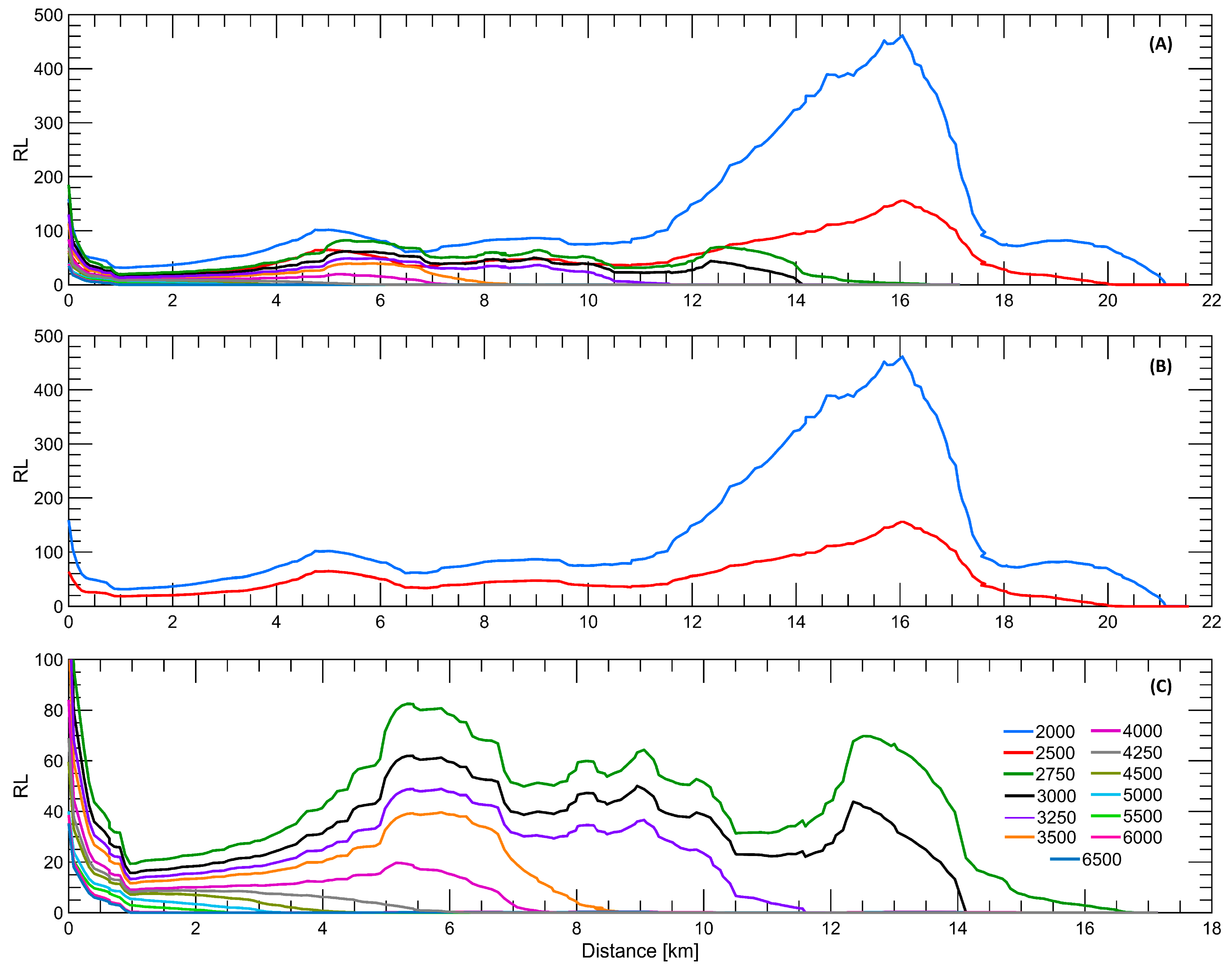
| Richardson Layered Number | It provides an estimate of the vertical mixture intensity by comparing the buoyant force and the shear stress. When RL < 2, the turbulence generated by friction is the main mixing mechanism. For 2 < RL < 20, the mixture becomes less effective. RL > 20 indicates that the water plot is stable and homogeneous. It is dimensionless [67]. |
| Turbulence Production * | This parameter assesses the production of bottom swirls because of the Reynolds stresses and the mean shear. Here, k is the Von Karman constant (0.41), z is the depth, is an alternative to expressing friction in terms of speed, and is the drag coefficient. It is measured in W/Kg [68]. |
| Month | Q (m3/s) | Qmin (m3/s) | Qmax (m3/s) | Qmax/Qmin (m3/s) |
|---|---|---|---|---|
| January | 6822 | 2326 | 13,844 | 5.95 |
| February | 4474 | 1705 | 10,074 | 5.91 |
| March | 4129 | 1520 | 8434 | 5.55 |
| April | 4938 | 2053 | 9951 | 4.85 |
| May | 6854 | 3402 | 12,892 | 3.79 |
| June | 8153 | 4667 | 14,475 | 3.10 |
| July | 7874 | 3132 | 14,425 | 4.61 |
| August | 7284 | 3109 | 13,063 | 4.20 |
| September | 7464 | 3214 | 13,196 | 4.11 |
| October | 8443 | 3699 | 13,920 | 3.76 |
| November | 9806 | 4594 | 16,913 | 3.68 |
| December | 9724 | 2916 | 16,913 | 5.80 |
| Flow Rate (m3/s) | Months with the Highest Probability of Occurrence | P. Accumulated (%) |
|---|---|---|
| 2000 ≤ Q ≤ 2500 | February and March | 7.2 and 7.7 |
| 2500 < Q ≤ 3000 | February and March | 12.9 and 16.7 |
| 3000 < Q ≤ 3500 | February, March, and April | 12.0, 16.7, and 10.7 |
| 3500 < Q ≤ 4000 | February, March, and April | 13.7, 11.9, and 11.0 |
| 4000 < Q ≤ 4500 | February, March, and April | 11.0, 11.7, and 14.3 |
| 4500 < Q ≤ 5000 | February, March, April, May, and September | 10.1, 10.1, 13.4, 6.6, and 6.3 |
| 5000 < Q ≤ 5500 | February, March, April, May, August, and September | 8.4, 7.8, 11.5, 9.5, and 6.5 |
| 5500 < Q ≤ 6000 | January, April, May, August, and September | 8.2, 10.4, 14.4, 10.1, and 6.9 |
| 6000 < Q ≤ 6500 | January, April, May, June, July, August, and September | 7.0, 8.2, 11.9, 7.3, 7.6, 11.2, and 10.7 |
| Q > 6500 | January, May, June, July, August, September, October, November, and December | 50.5, 54.3, 82.9, 72.6, 60.7, 64.1, 85.7, 95.5, and 90.1 |
| Month | Flow Rate (m3/s) | P. Accumulated (%) | NT-FSI | ST-FSI |
|---|---|---|---|---|
| December | 6000–14,583 | 90.1 | km < 2 | km < 2.2 |
| January | 3000–11,428 | 90.0 | km < 14.2 | km < 14.2 |
| February | 2500–8350 | 90.2 | km < 20.2 | km < 18.5 |
| March | 2000–6500 | 92.2 | km 1 and 21.1 | km 1.9 and 21.2 |
| April | 2500–6976 | 90.6 | km < 20.2 | km < 18.5 |
| May | 3500–8823 | 90.1 | km < 8.8 | km < 9.4 |
| June | 5000–10,909 | 91.0 | km < 3.4 | km < 3.6 |
| July | 3250–10,909 | 91.0 | km < 11.6 | km < 11.6 |
| August | 3250–10,243 | 90.0 | km < 11.6 | km < 11.6 |
| September | 3500–10,380 | 90.0 | km < 8.8 | km <9.4 |
| October | 5000–11,875 | 90.3 | km < 3.4 | km < 3.6 |
| November | 5500–13,215 | 90.3 | km < 2.5 | km < 3 |
| Month | Flow Rate (m3/s) | P. Accumulated (%) | NT-FSI | ST-FSI |
|---|---|---|---|---|
| December | 9800–10,334 | 93.7 | km ~ 0 | km ~ 0 |
| January | 2495–2917 | 88.9 | km 20.2 and 14.2 | km 18.5 and 14.2 |
| February | 2428–2507 | 89.6 | km ~ 20.2 | km ~ 18.5 |
| March | 2583–2780 | 90.3 | km 20.2 and 16.5 | km 18.5 and 16.6 |
| April | 2760–4054 | 90 | km 16.5 and 7.6 | km 16.6 and 7.6 |
| May | 4186–6155 | 90.3 | km 6 and 2 | km 6.5 and 2.2 |
| June | 5525–6306 | 90 | km 2.5 and 1 | km 3 and 1.9 |
| July | 4988–5548 | 90.3 | km 3.4 and 2.5 | km 3.6 and 3 |
| August | 4763–5884 | 90 | km 4.5 and 2 | km 5.5 and 2.2 |
| September | 5041–6573 | 90 | km 3.4 and 1 | km 3.6 and 1.9 |
| October | 6412–8177 | 90.3 | km < 1 | km < 1.9 |
| November | 8294–9650 | 90.0 | km ~ 0 | km ~ 0 |
Disclaimer/Publisher’s Note: The statements, opinions and data contained in all publications are solely those of the individual author(s) and contributor(s) and not of MDPI and/or the editor(s). MDPI and/or the editor(s) disclaim responsibility for any injury to people or property resulting from any ideas, methods, instructions or products referred to in the content. |
© 2024 by the authors. Licensee MDPI, Basel, Switzerland. This article is an open access article distributed under the terms and conditions of the Creative Commons Attribution (CC BY) license (https://creativecommons.org/licenses/by/4.0/).
Share and Cite
Cordero-Acosta, J.R.; Otero Díaz, L.J.; Higgins Álvarez, A.E. Influence of Fluvial Discharges and Tides on the Salt Wedge Position of a Microtidal Estuary: Magdalena River. Water 2024, 16, 1139. https://doi.org/10.3390/w16081139
Cordero-Acosta JR, Otero Díaz LJ, Higgins Álvarez AE. Influence of Fluvial Discharges and Tides on the Salt Wedge Position of a Microtidal Estuary: Magdalena River. Water. 2024; 16(8):1139. https://doi.org/10.3390/w16081139
Chicago/Turabian StyleCordero-Acosta, Jhonathan R., Luis J. Otero Díaz, and Aldemar E. Higgins Álvarez. 2024. "Influence of Fluvial Discharges and Tides on the Salt Wedge Position of a Microtidal Estuary: Magdalena River" Water 16, no. 8: 1139. https://doi.org/10.3390/w16081139
APA StyleCordero-Acosta, J. R., Otero Díaz, L. J., & Higgins Álvarez, A. E. (2024). Influence of Fluvial Discharges and Tides on the Salt Wedge Position of a Microtidal Estuary: Magdalena River. Water, 16(8), 1139. https://doi.org/10.3390/w16081139