Abstract
Slope vegetation is a key component of soil erosion control. Rigid vegetation improves slope stability, while flexible vegetation reduces water velocity, and the combination of both improves erosion resistance; however, there are few studies on how the combination of rigid and flexible vegetation affects the hydraulic characteristics of slope flow. In order to investigate the effect of this combination on the hydraulic characteristics of slopes, a mathematical model of the coefficient of resistance under the cover of rigid–flexible vegetation was established by using theoretical analysis and indoor tests, and the indoor tests were conducted with different rigid–flexible vegetation combinations (single-row interlocking (IS), double-row interlocking (IT), upstream rigid–downstream flexible (RF), and bare slope (BS)). The results showed that the rigid–flexible vegetation combination had a significant effect on the slope water flow. With the increase in flow, the water depth and flow velocity of slope flow showed an increasing trend, the flow velocity of the bare slope was significantly larger than that of the vegetation-covered slope, and the value of the water depth increment of the vegetation-covered slope was 0.086~0.22 times that of the bare slope. The Reynolds number showed a good linear increasing relationship with flow rate, and with the gradual increase in flow rate and slope, the flow pattern gradually changed from slow flow to fast flow. When the slope was 2°, the drag coefficient increased and then decreased. The pattern of erosion reduction capacity was IS > RF > IT > BS. The results of this study provide strong theoretical support for understanding the mechanism of vegetation-controlled erosion and provide scientific guidance for optimizing vegetation design in the Loess Plateau region.
1. Introduction
The Loess Plateau region has experienced severe soil erosion problems for a long time due to its soil-specific sub-stability, porous structure, and water sensitivity [1]. Since slope flow is the main driving force of soil erosion in this region [2], an in-depth investigation of its flow characteristics and influencing factors is crucial for elucidating the mechanism of loess soil erosion. Slope flow is a thin layer of water that flows along the surface of a slope due to gravity after snowmelt, rainfall, and losses such as infiltration, depression filling, and vegetation interception [3]. It plays a crucial role in slope erosion and sedimentation processes [4], and its hydraulic characteristics directly affect the intensity of slope erosion and its spatial distribution characteristics [5]. However, the hydraulic characteristics of slope flow are, in turn, mainly influenced by factors such as vegetation cover, slope, and flow rate. Vegetation plays a key role in maintaining ecological balance and environmental cycles [6,7,8,9], and vegetation cover not only reduces the degree of runoff scouring but also directly stabilizes the soil, increases the resistance of slope runoff by reducing the intensity of turbulence [10], and, thus, significantly mitigates the risk of soil erosion [11]. In recent years, although many studies have explored the influence of vegetation on the hydraulic characteristics of slope runoff, the interaction mechanism between vegetation and slope runoff and soil erosion is still not clear enough under the specific environment of loess areas. Therefore, an in-depth investigation of the change rule of the hydraulic characteristics of vegetation slope runoff, revealing the soil erosion mechanism of slope runoff, is of great theoretical and practical value for reducing soil erosion in loess areas.
Recently, researchers [12,13,14,15] have extensively studied the hydrodynamic characteristics of slope flow under vegetation cover and have classified vegetation as rigid or flexible based on the flexibility of their stems; rigid plants are taller and less prone to bending under the influence of water flow, whereas flexible plants are shorter and have softer stems that are more likely to bend due to water flow [16]. In previous studies, rigid cylindrical poles were explicitly defined to represent tree or reed models [17]; grass vegetation was replaced with simulated grass for indoor tests. Studies on the effect of vegetation on slope flow dynamics have focused on several key aspects, including cover, vegetation type, stem diameter, slope, and inundation depth [18,19]. For example, the density of rigid vegetation is one of the key factors affecting the flow regime of slopes [20], and it directly determines the roughness of the slope surface: with the increase in vegetation cover, the slope velocity is correspondingly reduced, which decreases the water flow rate [21]. The stem diameter of rigid vegetation also exerts a significant drag effect on surface runoff [22], and the Darcy–Weisbach drag coefficient and vegetation stem diameter are proportional to the vegetation stem diameter, i.e., the larger the vegetation stem diameter, the greater the resistance to runoff [23], and rigid vegetation configured behind slopes is considered the best way to alter water flow conditions and reduce soil erosion [24]. When vegetation was submerged, the coefficient of water flow resistance was unusually sensitive to the change in flow regime [25], indicating that the presence of vegetation not only changed the physical characteristics of the slope but also significantly affected the kinetic characteristics of water flow. Further studies found a significant correlation between the flow resistance of slope runoff and flexible vegetation patterns, especially flexible vegetation with a low degree of fragmentation [26]. A study of field plot tests found that the flexible plant alfalfa has a significant effect on slope resistance [27], and a different study found that the low flexible vegetation zone established along a slope can affect the runoff volume and sand production in the slope gully system [28].
The influence of vegetation characteristics on slope flow resistance is a research topic that has received much attention. However, current research has mainly focused on the effect of the layout of a single vegetation type (e.g., rigid or flexible vegetation) on slope flow characteristics. In contrast, there are few studies on the effect of the rigid–flexible vegetation combination approach on slope flow. Although many experiments have investigated the expression of water flow resistance under vegetation cover, no unified expression has been developed to accurately describe the calculation of flow resistance on vegetated slopes. The objective of this study was to develop a computational model for the slope flow resistance coefficient under rigid–flexible vegetation cover and investigate in depth the effect of the rigid–flexible vegetation combination method on the hydraulic characteristics of slope flow. The results of this study will provide strong theoretical support for understanding the mechanism of vegetation erosion control and provide scientific guidance for optimizing vegetation design in the Loess Plateau region.
2. Study Area and Materials
The study area was located in Heifangtai, Yongjing County, Gansu Province, on the western edge of the Loess Plateau in Longxi (longitude 102°53′ to 103°39′, latitude 35°47′ to 36°12′), with an elevation ranging from 1539 m to 2841 m (Figure 1). The average multi-year rainfall in the area is 287.6 mm, evaporation is 1593.4 mm, and the average annual temperature is 9.9 °C, belonging to the semi-arid climate of the mesothermal zone. Heifangtai is located in the fourth basement terrace on the north bank of the Yellow River, and the stratigraphic structure is, from bottom to top, purple-red sandy mudstone of the Cretaceous Hekou Group, pebble layer and orange-red powdery clay of the Middle Pleistocene of the Quaternary system, and loess of the Upper Pleistocene system [29], with loess predominant in the surface layer. The physical indices of the soil [30] are shown in Table 1. The study area is sparsely vegetated, and the top layer of loess is subject to more severe hydraulic and gravity erosion.
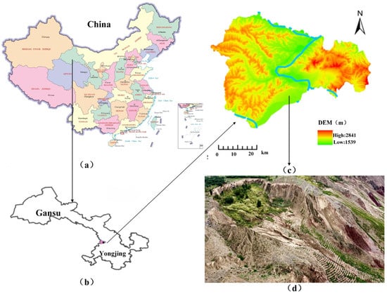
Figure 1.
(a,b) Study area; (c,d) current slope erosion management in the study area.

Table 1.
Basic physical property indices of loess in the project area.
The vegetation type of Yongjing County is semi-arid grassland, with common herbaceous plants such as wood grass and ice grass; planted forest species such as sea buckthorn, poplar, and willow; and artificially planted grasses such as alfalfa and awnless birdseed. However, the failure of existing engineering measures and the inappropriate selection of tree species and afforestation techniques have caused severe soil erosion [31]. As shown in Figure 1d, vegetation restoration measures were taken on loess slopes to mitigate slope erosion by planting trees with rigid and flexible herbaceous vegetation on the upper part of the slope, while flexible herbaceous vegetation was used on the lower part of the slope. However, the areas covered only with flexible herbaceous vegetation still experienced serious erosion problems, while no significant erosion was observed in the areas covered with a combination of rigid and flexible vegetation.
3. Methods and Experimental Design
3.1. Methodology
In this study, we adopted a combination of theoretical derivation and experimental study to systematically investigate the effects of the combination of rigid and flexible vegetation modes on the hydraulic characteristics of slope flow. Specifically, we first considered the difference in stem diameter between rigid and flexible vegetation and combined it with the consideration of drag coefficients [32,33] to conduct a comprehensive theoretical derivation of slope flow resistance coefficients using the force balance method. To visually demonstrate the mechanism of the influence of different rigid–flexible vegetation combinations on the hydraulic characteristics of slope flow, an indoor slope scour experiment was further designed and implemented [10,19]. The water depth and flow velocity data under different vegetation combinations were monitored in the experiment, and Excel 2021, such as analysis of variance (ANOVA) and regression analysis, was used to analyze the experimental data in depth. Finally, the change rule of hydraulic characteristics of slope flow was comprehensively and deeply analyzed by combining theoretical derivation and experimental data.
3.2. Scrub Test Design
This test was conducted in a flume laboratory using a self-constructed flume system consisting of a customized erosion system, flume, and water collection device. For this test, the erosion system was used to supply water, which consisted of a water storage tank, a constant head flushing device, water pipes, and a water pump (Figure 2a). The water tank was filled with water and the constant head was set at the top of the flume to ensure that the water flowed evenly into the flume. The catchment system consisted mainly of plastic containers placed at the bottom of the flume to collect the runoff. The dimensions of the test flume were 3 m × 0.3 m × 0.3 m. To study the effect of the spatial configuration of vegetation on the hydrodynamic characteristics of slope flow, 3 cm thick gravel with a diameter of 0~5 mm was placed at the bottom of the flume before the test; then, Q3 Malan loess with a thickness of 10 cm, which was collected from the study area, was placed at the top to simulate the conditions of the slope subsurface before the test [34] and ensure the practical feasibility of the test. The slope was divided into three slope sections from top to bottom, of which 0~1 m was the transition zone of water flow and the middle 1 m was the vegetation zone, and three measurement positions were set for each experiment from the top to the bottom of the flume, which were 0.5, 1.5, and 2.5 m, respectively. Each water depth was measured three times repeatedly to comprehensively understand the dynamic characteristics of the water flow of the slope (Figure 2b). The flow rate was controlled by a series of valves, with the water entering from the top of the tank. Five test flow rates were set considering the actual situation and combined with the test conditions, which were 0.25 L/s, 0.5 L/s, 1 L/s, 1.5 L/s, and 2 L/s. The test was set up with three different gentle slopes of 2°, 4°, and 6°, and the slopes and flow rates were adjusted to the design values before each test. The tank was filled with water and then the water in the tank was pumped through a water pipe to the constant tank above the flume; the water depth and flow rate measurements were made after the water flow had stabilized. The water depth was measured with a graduated scale with an accuracy of 0.1 mm, the discharge samples were collected with a plastic basin at the outlet of the flume every 5 min for each test, and the discharge temperature was measured with a thermometer to calculate the kinematic viscosity of the water flow.
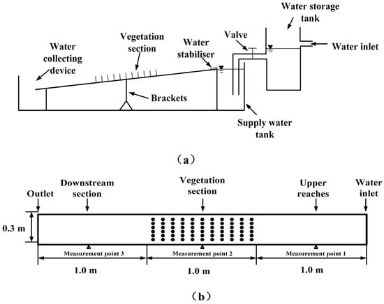
Figure 2.
Diagram of the test setup (a); diagram of the test configuration (b).
3.3. Rigid–Flexible Vegetation Design
Rigid and flexible vegetation was selected for testing. Round wooden sticks with a diameter of 6 mm were used to simulate the rigid plants (e.g., buckthorn, willow) in the study area in the natural state, with a vegetation height of 13.8 cm under the inundation condition, and plastic simulated grass was used to simulate the natural flexible grass vegetation (e.g., ice plant, timothy grass, alfalfa), with an average height of 5 cm under the inundation condition. The density of this test was designed to be 60 plants, and the combination of vegetation was set in four combinations: upstream rigid–downstream flexible, rigid–flexible single-row staggered, rigid–flexible double-row staggered, and bare slope (Figure 3).
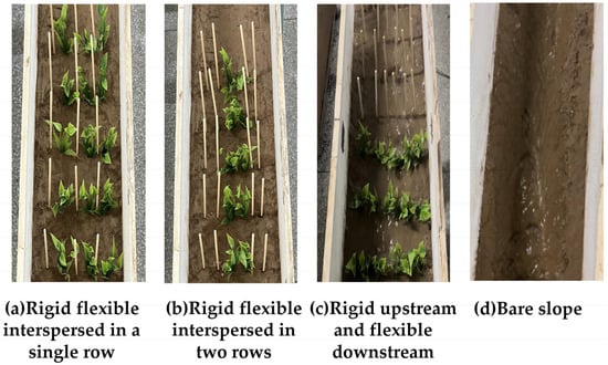
Figure 3.
Different combinations of rigid–flexible vegetation for IS (a), IT (b), RF (c), and BS (d).
4. Parameter Determination
To estimate the drag caused by vegetation, the force balance method was employed to calculate the drag coefficient in a uniform flow downstream of the vegetation area. The impact of sidewall friction was disregarded due to the shallow depth of the slope flow. The analysis primarily focused on the bypass drag (FD), bed surface shear stress (FB), and the gravitational effect of the water body on the slope surface (FW) induced by the vegetation. Combined with the calculation method of the equivalent composite coefficient of resistance of vegetation [35], a formula for the coefficient of resistance for the rigid–flexible vegetation cover was derived from the formula for calculating the coefficient of resistance under slope flow conditions.
The section of the flow in the vegetated area was selected for the force analysis and its combined resistance was calculated as follows:
In the formula provided, the variables represent various parameters related to water flow and vegetation within a control structure. These include the density of water (ρ) in g/cm3, the frictional flow velocity (v*) in m/s, the average flow velocity (v) in m/s, the total projected area of vegetation (Ap) in the direction of water flow in m2, the number of rigid (n1) and flexible (n2) vegetation plants within the structure, the diameters of the rigid (d1) and flexible (d2) vegetation in meters, the effective width of the cross-flow (B1) in meters, the length of the vegetation (L), the Darcy–Weisbach drag coefficient (f), the drag coefficient (CD), and the hydraulic gradient (J), with J = sin θ in the test:
where Cr is the vegetation cover and B is the width of the channel (m).
The coefficient of resistance to water flow in a thin layer on a slope, f, was calculated from the Darcy–Weisbach equation as
where R is the hydraulic radius, m; is the viscosity coefficient for water movement; and t represents the water temperature, °C.
Zeng Hongyu et al. [36] introduced the connection between the drag coefficient and the flow resistance coefficient:
where V is the volume of water in the control body.
Equations (1)–(5) could be obtained by association:
Assuming that the vegetation resistance was uniformly distributed over the bed, it was considered as particle resistance superimposed on the original bed to obtain an equivalent cross-section over water (Figure 4). In the figure, Ae is the post-equivalent cross-section over-water area, m2; H is the average height of the simulated grass cover, m; h is the average water depth of the cross section, m.
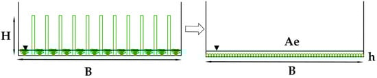
Figure 4.
Equivalent cross-section.
The flow rate before and after the equivalent transformation needed to be the same according to the continuity principle:
where ve represents the flow velocity and he stands for the water depth, as determined by the change in equivalence; Be denotes the effective spillway width.
According to the law of the conservation of mass for fluids, the volume of a body of water remains constant before and after any changes or transformations occur.
In this case, the volume of water in the vegetated section was as follows:
Then, the corresponding post-water depth was as follows:
The analysis of the forces of the equivalent sectional control body gave the following results:
Combining Formulae (1)–(3) and (14) gave
The equivalent coefficient of resistance of the slope flow could be obtained by combining Equations (7) and (15) as follows:
The above equation shows that the drag coefficient under vegetation cover fe = F(Cr, Re, J, h, L, λ), based on which the equivalent drag coefficient calculation model under rigid–flexible vegetation cover could be established:
In this study, coverage was a constant value. The above equation was simplified as follows:
where a is the combined coefficient of plant diameter (d1, d2), height H, and vegetation assemblage mode and b, c, and d are the influence indices of water depth, slope, and Reynolds number, respectively.
The rationality of the structure of the formula was verified with the Nash–Sutcliffe coefficient (NSE), calculated as
In the provided equation, Pi represents the simulated value, Oi represents the measured value, represents the average value of the measured values, and n is the number of samples.
5. Results
5.1. Changes in Water Depth and Slope Flow Velocity under Different Combinations of Rigid–Flexible Vegetation Cover
To deeply analyze the change characteristics of slope flow water depth and flow velocity under different combination approaches of rigid and flexible vegetation, the data were analyzed and processed using statistical analysis software, including ANOVA and regression analysis, through which the flow-affected water depth and flow velocity laws were revealed. Figure 5 shows the trend of water depth with flow, and the results show that there was an increasing power function relationship between slope flow water depth and flow (R2 > 0.98), which was obvious whether vegetation cover was present or not. With the increase in discharge, the slope flow water depth gradually increased, while, with the increase in slope, the water depth showed a decreasing trend. It is noteworthy that water depths were consistently greater on vegetated slopes than on BS. Vegetation cover had a significant regulating effect on slope water depth compared with BS; the value of water depth increment on vegetated slopes was 0.086 to 0.22 times that of BS and, under the same vegetation combination mode, with the increase in slope, the IS combination mode showed a better effect of water depth increment compared with other combination modes. To further verify the experimental results, the regression analysis of the experimental water depth (shown in Table 2) demonstrated that the coefficients of determination of the experimental values fitted with the regression results were R2 > 0.9, and the experimental values and the regression values both had a good positive correlation. This indicates that the experimental data of this study are reliable and the results have a high degree of confidence.
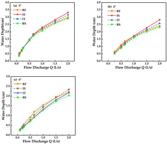
Figure 5.
Plot of discharge versus water depth at different gradients in order of gradient 2° (a), 4° (b), and 6° (c).
Table 2.
Relationship between flow and water depth at different slope gradients.
The results presented in Table 3 show the regression relationship between flow rate and flow velocity at different slope gradients, and the slope flow velocity tended to increase with increasing flow rate under the test conditions (R2 > 0.94). Figure 6 also shows the effect of vegetation cover on slope flow velocity. The rate of increase in slope flow velocity was slower on vegetated slopes. As the flow increased, the difference between the vegetation combination methods gradually decreased, and the average flow velocity on vegetated slopes decreased by 8.6~21.9% compared to that for BS. The variation observed may be linked to the extent of inclination of the vegetated slopes, where the presence of vegetation alters the shape of the slopes and consequently impacts the flow patterns. With the rise in flow velocity, both the vegetated and unvegetated slopes experienced an increase in average flow rates.
Table 3.
Relationship between flow rate and flow velocity at different slope gradients.
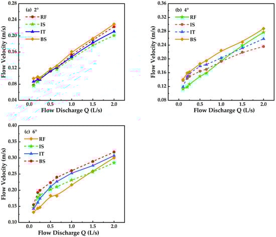
Figure 6.
Plots of flow rate versus flow velocity for slopes of 2° (a), 4° (b), and 6° (c).
To gain a deeper understanding of the effects of different vegetation assemblages on slope flow, an analysis of variance (ANOVA) was performed for flow, flow rate, and slope (as shown in Table 4). The results of this study revealed a notable distinction (p < 0.05) among the three vegetation combination techniques, RF, IS, and IT, regarding slope and flow velocity. This suggests that various vegetation combination methods significantly influence slope flow velocity. In similar flow conditions, the flow velocity of a bare slope (BS) was substantially higher than that of a slope covered with vegetation. The impact of different vegetation combinations on slope flow velocity followed the order of IS > IT > RF > BS, providing further evidence of the significant regulatory impact of vegetation combinations on flow velocity. It was also observed that there was no significant difference in water flow velocity between different slope sections on vegetated slopes, with slopes ranging from 2° to 6° and with a length of 1 m. This suggests that on natural slopes, the potential energy of water flow is mainly used to overcome surface roughness and vegetation resistance, and the kinetic energy of water flow is kept stable throughout the slope. However, in the experiment, the water flow velocity on the lower slope was higher than that on the higher slope, which may have been due to the different methods of vegetation combination. In this study, the vegetation was uniformly distributed throughout the slope, whereas, in natural slopes, the vegetation is usually unevenly distributed, and this unevenness may affect the kinetic characteristics of water flow, which may affect the velocity of water flow on the whole slope.
Table 4.
Analysis of variance (ANOVA) for bathymetry, flow velocity, and flow rate.
5.2. Changes in Slope Flow Patterns Based on Different Combinations of Rigid–Flexible Vegetation Cover
The Reynolds number plays a crucial role in determining the flow characteristics of slope flow, serving as an indicator of fluid flow properties. By applying the principles of open channel flow, the flow of water can be categorized into laminar, transitional, and turbulent zones. In particular, when the Re is less than 500, the water flow is in a laminar state; between 500 and 5000, it transitions to a turbulent state; and when Re exceeds 5000, the flow becomes turbulent. Figure 7 illustrates the change in the Reynolds number of the slope flow based on experimental conditions. This number ranged from a minimum of 292 to a maximum of 5847 as the flow increased. The flow was dominated by the transitional flow, and the Reynolds number increased on the vegetated slopes compared to the BS slopes. This may have been due to the presence of vegetation (e.g., logs), which altered the distribution pattern of runoff on the slopes. In particular, under the influence of vegetation, water flow was mainly concentrated in the area in front of and on both sides of the tree trunks, and this phenomenon may have contributed somewhat to the erosive effect in the non-vegetated area. The regression and ANOVA showed that there was a significant positive correlation between the Reynolds number and flow rate and a good linear increasing trend (R2 > 0.99). As the flow rate increased, the turbulence of the water flow increased, which indicated that the flow rate was the main factor affecting the Reynolds number. The analysis also showed that the effect of vegetation mix on the Reynolds number was not significant (p > 0.05).
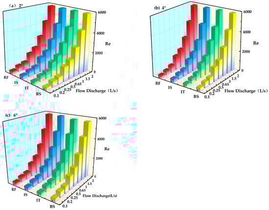
Figure 7.
Flow versus Reynolds number, in order of slope 2° (a), 4° (b), and 6° (c).
The Froude number, a key index for describing the flow pattern of water, reveals the relationship between the inertia of a water flow and its gravity. In open channel flow, the discrimination criterion states that when the Froude number (Fr) exceeds 1, the water flow exhibits rapid flow; when the Fr is less than 1, this indicates a slow flow; and when the Fr equals 1, the water flow reaches a critical state. Figure 8 shows that under the test flow rate, the slope flow presented as a slow flow state, and the Froude number was between 0.3 and 1.02. With the increase in flow rate, the slope Froude number exhibited a decreasing trend (R2 > 0.94), that is, the slope had a significant effect on the flow rate; the Froude number of the vegetated slopes was smaller than that of the bare slope, indicating that the presence of vegetation could effectively reduce the slope Froude number. As the slope increased, the Froude number increased significantly; the vegetated slopes increased the Froude number by about 50% compared with the BS, and the effect on the Froude number was significant between different vegetation combination methods, for which the Froude number of the RF combination method was higher than that of the IS and IT combination methods, indicating that the spread of the RF combination method had a weaker ability to block the runoff. To investigate the correlation between Froude number and vegetation combination techniques in greater depth, an analysis of variance (ANOVA) was performed to examine the Froude number across various vegetation combination methods. The findings illustrated a notable discrepancy (p < 0.05) in the Froude number among the different vegetation combinations, with the order of slope Froude number being RF > IS > IT. The reason for this difference could be that the vegetation distribution on the IS and IT slopes was more fragmented on the exposed slopes, whereas the exposed slopes were concentrated in the RF combination method, and the water flow through the unvegetated slopes had less resistance to flow and was more turbulent.
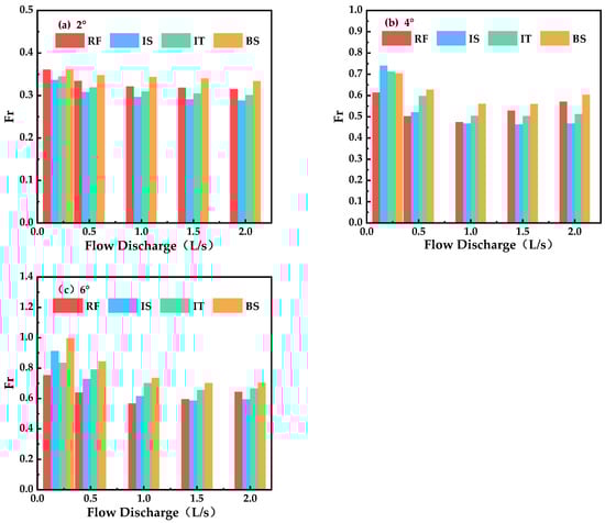
Figure 8.
Flow rate versus Froude number for slopes of 2° (a), 4° (b), and 6° (c), in this order.
5.3. Variation in Slope Flow Resistance Coefficient Based on Different Vegetation Combinations
5.3.1. Effect of Flow Rate on Drag Coefficient
The drag coefficient, f, reflects the amount of resistance the subsurface provides to flowing water. Under the same flow and slope conditions, an increase in the value of f means an increase in the amount of energy used by the water flow to overcome the resistance, which, in turn, reduces the amount of energy used for erosion and sediment transport and ultimately reduces the degree of soil erosion. In this study, tests were conducted at slopes of 2°, 4°, and 6° to obtain resistance coefficients ranging from 1.1 to 3.34, 0.66 to 2.78, and 0.8 to 2.53, respectively. Figure 9 shows the relationship between drag coefficients and flow rates under different vegetation mix conditions. Under the condition of a 2° slope, the drag coefficients of the IS and IT combinations tended to increase with the increase in flow rate as the slope gradually increased, while the drag coefficient of the RF combination method tended to decrease after increasing to a certain value. Overall, the resistance coefficients of each vegetation combination increased with the flow rate as the slope increased (R2 > 0.93). In addition, the resistance coefficients were greater for the vegetated slopes compared to the BS, indicating that slope flow had to overcome greater resistance and expend more energy in the vegetated conditions. Notably, the IT combination had the smallest coefficient of resistance to slope flow, indicating relatively poor erosion resistance.
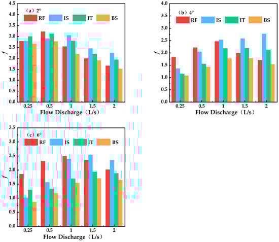
Figure 9.
Plots of flow rate versus drag coefficient for slopes of 2° (a), 4° (b), and 6° (c), in this order.
Regression analysis of the resistance coefficients of each group showed that the vegetation combination mode had the most significant effect on the resistance coefficients (p < 0.005). However, when the correlation test between flow rate and resistance coefficient was conducted under different vegetation combinations, we found that the absolute values of the correlation coefficients between them were all greater than 0.05, indicating that resistance coefficient and flow rate did not show obvious patterns of change under different vegetation combinations. This phenomenon can be attributed to the mixing and blending effect of the water flow in the vegetation, which caused the resistance coefficient not to significantly correlate with the flow rate. Taken together, the average drag coefficients at each flow rate were as follows: RF > IS > IT > BS.
5.3.2. Influence of Flow Pattern and Flow Regime on the Drag Coefficient
The resistance coefficient versus Reynolds number for slopes covered with different vegetation combinations is shown in Figure 10. This study indicated that the slope flow resistance coefficients exhibited a consistent trend across various vegetation combination methods. Overall, the coefficient of resistance values of the slopes of these four different vegetation combinations showed a power function increasing trend (R2 > 0.95) with the increase in the Re. When gradually increasing the Reynolds number and slope, the water flow tended to become turbulent, resulting in the weakening of the water resistance effect of the vegetation, which gradually lowered the rate of increase of the resistance coefficient.
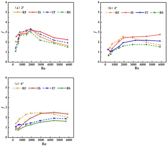
Figure 10.
The plot of Reynolds number versus drag coefficient in order of slopes of 2° (a), 4° (b), and 6° (c).
5.3.3. Influence of Froude Number on the Integrated Drag Coefficient
To further investigate the trends of the drag coefficient under different flow regimes and the influence of vegetation on the hydraulic characteristics of slope flow, regression analyses were performed on the drag coefficient of the slope flow and Froude number. Figure 11 showed that the drag coefficient showed a logarithmic decreasing trend (R2 > 0.95) with the increase in the Froude number. In addition, the effect of the Froude number on the drag coefficient varied at different slopes, which was realized as the absolute value of the power index of the Froude number, which increased from 1.85 to 2.41. Further investigation of the effect of different vegetation combinations on the correlation between the drag coefficient and the Froude number revealed that the correlation between the drag coefficient of slope flow and the Froude number was weakened under the vegetation cover condition compared to the BS condition. This result can be attributed to the presence of vegetation, which caused the water flow to appear inhomogeneous in terms of flow direction and velocity, resulting in the difference in this relationship.
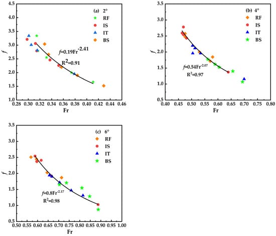
Figure 11.
Plots of Froude number versus drag coefficient for slopes of 2° (a), 4° (b), and 6° (c) sequentially.
5.4. Model Validation
In summary, the slope vegetation resistance was closely related to the Reynolds number, water depth, and slope obtained by fitting the experimental data to the constructed model:
The importance of the absolute value of the index for each factor in Equation (23) indicated the impact of its variation on the drag coefficient. This suggested that the influence of each factor on the drag coefficient was strongly linked to the flow regime. The analysis revealed that water depth plays a primary role in determining the integrated drag coefficient, followed by the Reynolds number.
The Nash–Sutcliffe coefficient was utilized to assess the simulation accuracy of the drag coefficient calculation model; the closer the NSE value was to 1, the better the model simulation effect was. The calculated NSE value was 0.762, so the model could better simulate the calculation of the integrated drag coefficient of slope flow under the staggered cover of rigid–flexible vegetation. After analyzing the calculated values of the model and comparing them with the Darcy–Weisbach drag coefficient values, it was determined that both sets of data aligned well. The data points were closely distributed along the 1:1 line, confirming that the model effectively matched the experimental data. Figure 12 further validates the accuracy and reliability of the fitted formula.
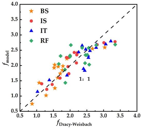
Figure 12.
Comparison of the Darcy–Weisbach drag coefficients with those predicted using Equation (23).
6. Discussion
6.1. Influence of Vegetation Cover and Slope on the Hydraulic Characteristics of Slope Flow
Vegetation cover has a significant effect on slope runoff [37]: it profoundly affects erosion, sediment transport, and deposition processes by changing the hydrological characteristics of slope runoff [38]. Based on a review of related studies, we found the following: Vegetation cover plays a key role in reducing the direct impact of raindrops on soil and lowering the soil erosion rate [39]; it not only affects the onset time, flow rate, and runoff volume of slope runoff but is also directly related to the change in soil erosion rate [13]. Vegetation is an effective approach to combating erosion [40]. In this study, the effect of vegetation on runoff flow rate was relatively small on slopes with a small gradient when vegetation cover was kept constant; however, as the gradient increased, the inhibitory effect of vegetation on runoff flow rate became more significant. This is consistent with other findings on the relationship between slope and erosion and hydraulic characteristics [41], and it was also observed that water flow was slow on all slopes. Furthermore, it was found that vegetation effectively increases resistance to water flow by increasing the energy consumed by the water flow, thus reducing the amount of sediment [8]. In summary, the effect of vegetation cover on slope flow is multifaceted and significantly affects the process of slope erosion and sediment transport by changing the characteristics of water velocity, morphology, and resistance. To deeply understand this influence mechanism, we need to comprehensively consider factors such as vegetation type, combination mode, slope, and soil type. This study also considered the differences between rigid and flexible vegetation in terms of drag force, emphasizing the importance of this force in mathematical models of slope flow, which can be used to more accurately predict and evaluate the influence of vegetation cover on the hydraulic characteristics of slope flow by continuously refining and improving these models.
6.2. Effect of Rigid and Flexible Vegetation on the Hydraulic Characteristics of Slope Flows
Rigid vegetation and flexible vegetation showed significant differences in their influence on the hydraulic characteristics of slope flow. First, for rigid vegetation, the resistance to slope flow was greater because of its structural stability, especially in the flow rate, Reynolds number, and water depth increase; the total energy in the longitudinal position compared to bare slopes showed a fluctuating downward trend [24], indicating a stronger buffer capacity, which is conducive to reducing slope erosion and enhancing soil and water conservation. Moreover, rigid vegetation stem diameter exhibited significant resistance to surface runoff [22], and the resistance increased with increasing stem diameter [23]. By contrast, flexible vegetation exhibited the phenomena of bending, inverting, and deflecting under the action of water flow, and these dynamic changes further complicated the influence of flexible vegetation on the hydraulic characteristics of slope flow. The average flow rate under flexible vegetation cover was more easily affected by the water flow; in particular, with the increase in rainfall intensity, the distribution pattern of flexible grass cover at the top of the slope, the middle of the slope, and the bottom of the slope has a gradually weakening effect on the flow rate [42]. In addition, the flow rate of the grass-covered section was lower than that of the bare section, and the flow rate of the downslope section was significantly larger than that of the upslope section [43]. Therefore, the combination of vegetation plays a key role. For example, the reasonable ratio of rigid and flexible vegetation showed a significant effect in controlling soil erosion, where soil loss on the slope was minimized when the ratio of rigid and flexible vegetation was 1:2 [44]. The results of this study showed that in the process of runoff flow through the slope, as the flow rate increased, the slope runoff flow rate increased more and more slowly, in which the bare slope and the upstream rigid—downstream flexible flow rate were the highest, followed by the combination of double-row staggered and single-row staggered modes. With the gradual increase in the Reynolds number (Re), the flow state gradually transitioned from stable laminar flow to turbulent flow, and this process was accompanied by a significant increase in the flow resistance coefficient. This observation is in agreement with those of previous studies [45]. Therefore, only a multifaceted study of the relationship between vegetation and slope flow can provide a deeper understanding of the mechanisms of soil erosion [46].
6.3. Proposals for the Future
Current research focuses on single vegetation types such as rigid plants (shrubs) or flexible plants (grasses), but little research has been conducted on the effects of combining rigid and flexible plant cover on soil erosion. Rigid and flexible plants each have unique mechanisms for reducing runoff and sediment production. Therefore, to fully utilize the benefits of vegetation in reducing runoff and soil erosion, it is necessary to study in depth more effective methods of vegetation combination. This will provide important theoretical support and practical guidance for optimizing vegetation layout in loess areas. It is suggested that follow-up research should further expand this field to promote the in-depth development of related ecological restoration and management.
7. Conclusions
In this study, we investigated changes in slope flow hydrodynamic characteristics for four different combinations of rigid and flexible vegetation (RF, IS, IT, and BS) at different flow rates by using theoretical analysis and indoor experiments. The main conclusions are as follows:
(1) A resistance model was constructed that integrates the effects of slope and the Reynolds number, providing theoretical support for the hydrodynamic characterization of slope flow with a rigid–flexible combination of vegetation cover.
(2) Different combinations of rigid and flexible vegetation have significant effects on water depth, discharge, Froude number, and drag coefficient on the slope. Water depth, discharge, and velocity are closely related (R2 > 0.98). When comparing different vegetation combinations, the IS combination has superior performance: it can effectively raise water levels, reduce the flow rate, and enhance the effect of soil and water conservation. The Reynolds number of vegetated slopes was higher than that of the bare slope and increased linearly with increasing flow (R2 > 0.99). The Froude number decreased with increasing flow, and the resistance coefficient was negatively correlated with the Froude number, in which the water flow turbulence of the slope with the IS combination was less.
(3) The flow resistance coefficients for the vegetated slopes ranged from 0.66 to 3.34, with the IS combination having the highest resistance and the IT combination having the lowest resistance. The combined drag coefficient of each combination increased with increasing flow rate and Reynolds number (R2 > 0.93). For vegetation restoration in the Yellow River basin, the rigid–flexible vegetation IS combination is a better choice.
Author Contributions
The research idea was proposed by L.X. Manuscript writing was performed by H.T. and F.W. The experiments were operated by Z.B. and D.Z. Data were processed by S.B. and X.S. All authors have read and agreed to the published version of the manuscript.
Funding
This study was supported by the Mechanical Mechanism of Instability of Shock-Damaged Loess Landslide Based on Spatial Structure Differences project (52360031), Gansu Province Higher Education Institutions Industrial Support Program project (2022CYZC-32), Technological Innovation Guidance Program—Special Project for Science and Technology Commissioner (23CXGA0074), and the Gansu Provincial Water Conservancy Science and Technology Promotion Program project “Research on Bioforestation Technology for Efficient Utilization of Rainfall-Runoff in Lanzhou New Area” (Gan Shui Ke Wai Fa (2018) no. 70).
Data Availability Statement
The data in this study were the basis for the analysis that we performed.
Conflicts of Interest
The authors declare no conflicts of interest.
References
- Xie, X.; Li, P.; Hou, X.; Li, T.; Zhang, G. Microstructure of compacted loess and its influence on the Soil-Water characteristic curve. Adv. Mater. Sci. Eng. 2020, 2020, 3402607. [Google Scholar] [CrossRef]
- Zhu, H.; Zhao, Y.; Liu, H. Scale characters analysis for gully structure in the watersheds of loess landforms based on digital elevation models. Front. Earth Sci. 2018, 12, 431–443. [Google Scholar] [CrossRef]
- Zhang, K.; Wang, Z.; Wang, G.; Sun, X.; Cui, N. Overland-Flow resistance characteristics of nonsubmerged vegetation. J. Irrig. Drain. Eng. 2017, 143, 04017021. [Google Scholar] [CrossRef]
- Qin, W.; Cao, W.; Guo, Q.; Yu, Y.; Yin, Z. Review of the effects of vegetation patterns on soil erosion and sediment yield. Acta Ecol. 2017, 37, 4905–4912. [Google Scholar]
- Zhang, J.; Zhang, S.; Chen, S.; Liu, M. Effects of sparse rigid stem vegetation coverage on hydrodynamic characteristics of overland flow in a gentle slope area. Arab. J. Geosci. 2021, 14, 1445. [Google Scholar] [CrossRef]
- Wang, W.; Huai, W.; Zeng, Y.; Zhou, J. Analytical solution of velocity distribution for flow through submerged large deflection flexible vegetation. Appl. Math. Mech. 2015, 36, 107–120. [Google Scholar] [CrossRef]
- Zhang, S.; Zhang, J.; Liu, Y.; Liu, Y. Effects of farmland vegetation row direction on overland flow hydraulic characteristics. Hydrol. Res. 2018, 49, 1991–2001. [Google Scholar] [CrossRef]
- Ding, W.; Li, M. Effects of grass coverage and distribution patterns on erosion and overland flow hydraulic characteristics. Environ. Earth Sci. 2016, 75, 477. [Google Scholar] [CrossRef]
- Zhou, Z.; Li, X.; Chen, L.; Li, B.; Liu, T.; Ai, B.; Yang, L.; Liu, B.; Chen, Q. Macrobenthic assemblage characteristics under stressed waters and ecological health assessment using AMBI and M-AMBI: A case study at the Xin’an River Estuary, Yantai, China. Acta Oceanol. Sin. 2018, 37, 77–86. [Google Scholar] [CrossRef]
- Zhao, C.; Gao, J.; Huang, Y.; Wang, G.; Zhang, M. Effects of vegetation stems on hydraulics of overland flow under varying water discharges. Land Degrad. Dev. 2016, 27, 748–757. [Google Scholar] [CrossRef]
- Sun, J.; Zhang, L.; Zhao, L.; Pan, X.; Lei, X.Z. Experimental study of the effects of different height flexible vegetation on hydraulic characteristics of overland flow. Mech. Eng. 2016, 38, 283–289. [Google Scholar]
- Luo, M.; Pan, C.; Peng, J.; Wang, L. Characteristics of the sediment transport process in vegetation hillslopes under different flow rates. Water 2023, 15, 2922. [Google Scholar] [CrossRef]
- Han, D.; Deng, J.; Gu, C.; Mu, X.; Gao, P.; Gao, J. Effect of shrub-grass vegetation coverage and slope gradient on runoff and sediment yield under simulated rainfall. Int. J. Sediment Res. 2021, 36, 29–37. [Google Scholar] [CrossRef]
- Wang, L.; Zhang, Y.; Jia, J.; Zhen, Q.; Zhang, X. Effect of vegetation on the flow pathways of steep hillslopes: Overland flow plot-scale experiments and their implications. Catena 2021, 204, 105438. [Google Scholar] [CrossRef]
- Peng, Q.; Liu, X.; Huang, E.; Yang, K. Experimental study on the influence of vegetation on the slope flow concentration time. Nat. Hazards 2019, 98, 751–763. [Google Scholar] [CrossRef]
- Zhang, K.; Jing, H.F.; Song, Y.T.; Li, C.G. Experimental study on flow characteristics in a flume with flexible vegetation. Yangtze River 2018, 49, 97–102. [Google Scholar]
- Tang, H.; Tian, Z.; Yan, J.; Yuan, S. Determining drag coefficients and their application in modelling of turbulent flow with submerged vegetation. Adv. Water Resour. 2014, 69, 134–145. [Google Scholar] [CrossRef]
- Zhang, Y.X.; Ma, L.; Xue, M.H.; Sun, X.; Wang, F.X.; Li, H.Y.; Song, T.Y. Experimental study on hydraulic characteristics of overland flow under different surface roughness. J. Shaanxi Norm. Univ. (Nat. Sci. Ed.) 2023, 51, 1–10. [Google Scholar]
- Zhang, S.; Zhang, J.; Liu, Y.; Liu, Y.; Wang, Z. The effects of vegetation distribution pattern on overland flow. Water Environ. J. 2018, 32, 392–403. [Google Scholar] [CrossRef]
- Pasha, G.A.; Tanaka, N. Critical resistance affecting sub- to Super-Critical transition flow by vegetation. J. Earthq. Tsunami 2019, 13, 1950004. [Google Scholar] [CrossRef]
- Zhao, C.; Gao, J.; Zhang, M.; Wang, F.; Zhang, T. Sediment deposition and overland flow hydraulics in simulated vegetative filter strips under varying vegetation covers. Hydrol. Process. 2016, 30, 163–175. [Google Scholar] [CrossRef]
- Zhang, S.; Zhang, J.; Liu, Y.; Liu, Y.; Li, G. The resistance effect of vegetation stem diameter on overland runoff under different slope gradients. Water Sci. Technol. 2018, 78, 2383–2391. [Google Scholar] [CrossRef] [PubMed]
- Zhang, J.; Zhang, S.; Wang, C.; Wang, W.; Ma, L. Influence of combined stem vegetation distribution and discretization on the hydraulic characteristics of overland flow. J. Clean. Prod. 2022, 376, 134188. [Google Scholar] [CrossRef]
- Wang, Y.; Zhang, H.; Yang, P.; Wang, Y. Experimental study of overland flow through rigid emergent vegetation with different densities and location arrangements. Water 2018, 10, 1638. [Google Scholar] [CrossRef]
- Cantalice, J.R.B.; Melo, R.O.; Silva, Y.J.A.B.; Cunha Filho, M.; Araújo, A.M.; Vieira, L.P.; Bezerra, S.A.; Barros, G.; Singh, V.P. Hydraulic roughness due to submerged, emergent and flexible natural vegetation in a semiarid alluvial channel. J. Arid Environ. 2015, 114, 1–7. [Google Scholar] [CrossRef]
- Zhao, Q.; Zhang, Y.; Xu, S.; Ji, X.; Wang, S.; Ding, S. Relationships between riparian vegetation pattern and the hydraulic characteristics of upslope runoff. Sustainability 2019, 11, 2966. [Google Scholar] [CrossRef]
- Sun, Y.; Liu, X.Y.; Tian, Y.; Zhang, X.; Fan, X.G.; Cui, Q.L. Experimental Study on the Response Characteristics of Flow-Sediment Transport on Slope to the Vegetation Coverage. J. Basic Sci. Eng. 2020, 28, 632–641. [Google Scholar]
- Huo, Y.P.; Zhu, B.B. Experimental Study on Impacts of Vegetation Patterns on Sediment Yield of Slope. Res. Soil Water Conserv. 2022, 29, 14–20. [Google Scholar]
- Wu, W.J.; Su, X.; Ye, W.L.; Wei, W.H.; Yang, T.; Feng, L.T. Lateral pressure in formation of saturated loess landslide—Case study of Heifangtai, Gansu Province. Chin. J. Geotech. Eng. 2018, 40, 135–140. [Google Scholar]
- Tao, H.; Lei, S.; Gong, L.; Shi, X.; Zhang, M.; Yang, G. Study on erosion and stability of the ecological slope. Front. Earth Sci. 2023, 10, 1071231. [Google Scholar] [CrossRef]
- Li, Y.B. Problems and countermeasures of comprehensive soil and water loss management in Yongjing county, Gansu province. Beijing Agric. 2015, 17, 69–70. [Google Scholar]
- Wu, F.C.; Shen, H.W.; Chou, Y.J. Variation of roughness coefficients for unsubmerged and submerged vegetation. J. Hydraul. Eng. 1999, 125, 934–942. [Google Scholar] [CrossRef]
- Crompton, O.; Katul, G.G.; Thompson, S. Resistance formulations in shallow overland flow along a hillslope covered with patchy vegetation. Water Resour. Res. 2020, 56, e2020WR027194. [Google Scholar] [CrossRef]
- Dong, X.; Zhang, K.D.; Yang, M.Y.; Gao, Y.L.; Ma, X.L. Dynamics characteristics of rill flow on loess slope. Sci. Soil Water Conserv. 2016, 14, 45–51. [Google Scholar]
- Jiang, B.H.; Yang, K.J.; Cao, S.Y.; Chen, L. Modeling the velocity distribution in compound channels with vegetated floodplains based on the equivalent resistance. Shuili Xuebao 2012, 43, 20–26. [Google Scholar]
- Zeng, H.Y.; Huai, W.X.; Zhang, J.; Li, Q.B. Flow resistance of emerged rigid vegetations in open channels. Shuili Xuebao 2011, 42, 834–838+847. [Google Scholar]
- Zhao, X.; Chen, X.; Huang, J.; Wu, P.; Helmers, M.J. Effects of vegetation cover of natural grassland on runoff and sediment yield in loess hilly region of China. J. Sci. Food Agric. 2014, 94, 497–503. [Google Scholar] [CrossRef]
- Zhang, G.; Liu, G.; Yi, L.; Zhang, P. Effects of patterned Artemisia capillaris on overland flow resistance under varied rainfall intensities in the Loess Plateau of China. J. Hydrol. Hydromech. 2014, 62, 334–342. [Google Scholar] [CrossRef]
- Rehman, O.U.; Rashid, M.; Kausar, R.; Alvi, S.; Hussain, R. Slope gradient and vegetation cover effects on the runoff and sediment yield in hillslope agriculture. Turk. J. Agric. Food Sci. Technol. 2015, 3, 478–483. [Google Scholar] [CrossRef][Green Version]
- Madi, H.; Mouzai, L.; Bouhadef, M. Plants Cover Effects on Overland Flow and on Soil Erosion under Simulated Rainfall Intensity. Int. J. Environ. Ecol. Eng. 2013, 7, 561–565. [Google Scholar]
- An, J.; Zheng, F.; Lu, J.; Li, G. Investigating the role of raindrop impact on hydrodynamic mechanism of soil erosion under simulated rainfall conditions. Soil Sci. 2012, 177, 517–526. [Google Scholar] [CrossRef]
- Xiao, P.Q.; Yao, W.Y.; Shen, Z.Z. Experimental study on erosion process and hydrodynamics mechanism of alfalfa grassland. Shuili Xuebao 2011, 42, 232–237. [Google Scholar]
- Zhang, G.; Hu, J. Effects of patchy distributed Artemisia capillaris on overland flow hydrodynamic characteristics. Int. Soil Water Conserv. Res. 2019, 7, 81–88. [Google Scholar] [CrossRef]
- Ren, K.M.; Wei, W.; Zhao, X.N.; Feng, T.J.; Chen, D.; Yu, Y. Simulation of the effect of slope vegetation cover and allocation pattern on water erosion in the loess hilly region. Acta Ecol. Sin. 2018, 38, 8031–8039. [Google Scholar]
- Shen, H.; Zheng, F.; Wen, L.; Han, Y.; Hu, W. Impacts of rainfall intensity and slope gradient on rill erosion processes at loessial hillslope. Soil Tillage Res. 2016, 155, 429–436. [Google Scholar] [CrossRef]
- Igwe, P.U.; Ezeukwu, J.C.; Edoka, N.E. A review of vegetation cover as a natural factor to soil erosion. Int. J. Rural. Dev. Environ. Health Res. 2017, 1, 21–28. [Google Scholar]


Disclaimer/Publisher’s Note: The statements, opinions and data contained in all publications are solely those of the individual author(s) and contributor(s) and not of MDPI and/or the editor(s). MDPI and/or the editor(s) disclaim responsibility for any injury to people or property resulting from any ideas, methods, instructions or products referred to in the content. |
© 2024 by the authors. Licensee MDPI, Basel, Switzerland. This article is an open access article distributed under the terms and conditions of the Creative Commons Attribution (CC BY) license (https://creativecommons.org/licenses/by/4.0/).