Abstract
While studies have shown that heavy metal sulfides in sediments are not bioavailable, most of them are acid-extractable (AE) and inseparable from non-sulfides in sediments. Exceptions were found recently that mercury and copper sulfides precipitated in sediments are non-AE because they are exclusively bi-sulfides. Therefore, quantifying mercury sulfide in sediments is possible for bioavailability assessment. To illustrate the application of this new approach for mercury bioavailability assessment, we quantified the distribution of mercury sulfide in sediments of the Apalachicola Bay, North Florida, USA. We extracted sediment cores and determined the total mercury, non-sulfide mercury, and sulfide mercury as well as the total sulfides, bulk density, and organic matter. The results showed that the mercury in the top 45 cm sediments were, on average, 13.3 ± 5.4 ng/cm3, of which 97.1 ± 2.5% were sulfide. The potentially bioavailable (non-sulfide) mercury was on average only 0.28 ± 0.22 ng/cm3 (2.9% of the total mercury). The total mercury and sulfide mercury were significantly correlated with the organic matter, which were dictated by the discharge pattern of the river input. This study demonstrates that aquatic sediments accumulate terrestrial mercury, and sulfidic sediments sequester most of it as sulfide. This new approach for mercury bioavailability assessment is simple yet chemically rigorous.
1. Introduction
The potential of Hg entering the food chain in aquatic systems has been a public health concern for decades [1]. The bioavailable Hg in sediments, however, cannot be represented by the total Hg concentration [2,3]. Therefore, Hg bioavailability assessment in aquatic systems becomes a crucial issue. Most Hg found in fish is methylmercury (MeHg); therefore, MeHg has been an indicator of bioavailable Hg [4,5]. However, MeHg is only a fraction of the potentially bioavailable Hg, and the dynamic of Hg methylation/demethylation makes MeHg not a steady indicator [6]. Currently, Hg bioavailability is assessed by operationally defined methods such as sequential leaching or extractions [7,8,9]. Other than being tedious, what is actually extracted by these methods remains uncertain. For example, Na2S extraction is supposedly to extract Hg sulfide, which is non-bioavailable, but it may also contain HgCl2 and/or other non-sulfide Hg species that are not necessarily non-bioavailable [7]. Using operationally defined methods for Hg bioavailability assessment is ambiguous because they are not rigorously defined [9].
Studies have shown that heavy metals (HMs) in sulfide forms are non-bioavailable because they are highly insoluble in water [10,11,12,13,14,15]. However, most HM sulfides are mono-sulfides, which are acid (HCl)-extractable (AE), and inseparable from non-sulfide forms in sediments. A recent study [16], however, showed that mercury and copper sulfides precipitated in sediments are not mono-sulfides, but exclusively bi-sulfides, which are non-acid (HCl)-extractable (non-AE) under nitrogen. Mercury sulfide in sediments, therefore, can be analytically separated from non-sulfide forms and excluded from bioavailability assessments. Unlike the operationally defined extraction and leaching methods, this method of quantifying mercury sulfide is chemically rigorous, making it suitable for mercury bioavailability assessment in sediments.
To illustrate the application of this new approach, we assessed the mercury bioavailability in the sediments of Apalachicola Bay, North Florida, USA, by determining the distribution of mercury sulfide (non-AE) from its non-sulfide (AE) forms. We also determined the total sulfides, bulk density, and organic matter contents of the sediments. We investigated their relationships with the total mercury, sulfide mercury, and non-sulfide mercury in the sediments.
2. Materials and Methods
2.1. The Study Site
Apalachicola Bay, a bar-built estuary located in the northwestern coast of Florida, USA (Figure 1), is a highly productive system that supports an abundant recreational and commercial fishery [17]. The Apalachicola Bay system includes St. George Sound, East Bay and St. Vincent Sound, and is separated from the Gulf of Mexico by four islands: St. Vincent Island, Cape St. George, St. George Island, and Dog Island. Apalachicola Bay is approximately 63 km long,12 km wide, 2–3 m deep, and covers an area of around 539–542 km2 [17,18,19,20,21]. The average annual discharge of the Apalachicola River to the Bay between 1978 and 2016 was 38,640 m3/minute [22]. Freshwater and seawater inputs are derived mainly from the Apalachicola River and St. George Sound, respectively, with the former dominating over other currents in the bay. Water from the river disperses west of the Bay and exits to the Gulf of Mexico through the natural inlet West Pass [19]. Water exchanges with the Gulf also occur through natural inlets, including Indian Pass and East Pass, as well as artificial Sikes Cut, which separates the Cape St. George Island State Reserve from the western end of St. George Island.
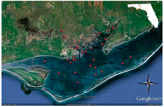
Figure 1.
Apalachicola Bay, North Florida, USA, and the 27 sediment sampling stations. The star indicates the location of Tallahassee, and the circle indicates the location of Apalachicola Bay. Only the data of the 25 stations close to or in the Bay were used in this report.
2.2. Sample Collection
Twenty-five (25) stations were selected for sediment sampling (Figure 1). Our sampling stations represented different hydrological zones all over the Bay and proximity to freshwater and saline water inputs. Sediment cores of four stations were collected in the Spring season those of the remaining 21 stations were collected during the summer season. Using a Russian corer, sediment cores up to 45 cm deep were extracted and sectioned into 5 cm intervals. Duplicate sediment cores or grabbed samples were collected for the sampling stations. The sectioned sediments were immediately sampled into plastic cut-off 20 mL syringes; excess headspace in the cut-off syringes was pushed out, and the sediments were sealed with rubber stoppers to prevent contact with air. Core samples were collected from nine (9) stations. Additional grab samples (approximately 0–20 cm depth) were collected from the other 16 stations. The grab sediments were also immediately subsampled into 20 mL cut-off plastic syringes and sealed with rubber stoppers. Samples in the syringes were stored in ice during transport to the laboratory and processed for moisture content, bulk density, acid volatile sulfide (AVS), chromium reducible sulfide (CRS or bi-sulfide), AE-Hg under nitrogen, and total Hg according to the detail described in the following sections.
2.3. Acid-Volatile-Sulfide (AVS) and Chromium-Reducible-Sulfide (CRS)
The AVS and CRS in the sediments were determined sequentially by the diffusion methods [23,24]. Briefly, 4–19 g wet weight (equivalent to 2–12 g dry weight) sample was taken from the cut-off syringes into a 300 mL distillation bottle. A 10 mL alkaline-Zn solution trap was inserted into the bottle and the bottle closed with a two-outlet stopper. The outlets were closed after the bottle was purged with pure nitrogen gas. The nitrogen purge flow rate was approximately 500 mL/minute. The purging time was about three minutes, enough to replace all the headspace air (300 mL) with nitrogen. Ten mL 6M HCl was injected through one of the outlets onto the sediment to liberate AVS as hydrogen sulfide, which was subsequently precipitated by the Zn-alkaline solution and quantified by iodometric titration [25]. After AVS, a 10 mL acidic Cr(II) solution was injected into the sediment in the nitrogen-filled bottle to determine the CRS, which is the sum of bi-sulfides and poly-sulfides.
2.4. Acid-Extractable (AE-Hg) and Total Hg (HgT)
AE-Hg extraction was conducted in a two-outlet-stoppered 300 mL bottle under nitrogen. Two to seven (2–7) g wet sample (1–4 g dry weight) were weighed into the bottle. After the bottle was purged with nitrogen, 10 mL 1M HCl (prepared from double-distilled HCl and water) was injected into the sediment through one of the outlets in the stopper. The bottle was shaken overnight (16–21 h), the supernatant was collected, and centrifuged (5000 rpm for 10 min). The supernatant solution was analyzed for Hg using cold vapor atomic fluorescence spectrophotometry (CVFAS).
HgT was measured directly using mercury analyzer DMA-80 (Milestone Inc., Shelton, CT, USA). Together with the samples, we also analyzed NIST Standard Reference Materials SRM 1570a Spinach leaves (0.030 ± 0.003 µg Hg/g) and SRM1515 Apple leaves (0.044 ± 0.004 µg Hg/g) as checks for the accuracy of the analysis. The results of measurements were 0.028 ± 0.002 µg Hg/g and 0.042 ± 0.003 µg Hg/g, respectively, for the SRM 1570a Spinach leaves and the SRM1515 Apple leaves. The non-AE-Hg was obtained from the difference between the HgT and the AE-Hg measurements. The DMA-80 detection limit is 0.005 ng Hg with a typical standard deviation of <1.5%. It has work ranges of 0–20 ng or 20–1000 ng. The DMA-80 requires a single-point calibration using either liquid or solid reference materials. If the blank has a peak height <0.02 (<0.005 ng Hg), instrument is considered free from contamination. Peak height values <0.02 are considered non-detectable. The coefficient of variation is 4.3–15.5% for duplicated sediment samples.
2.5. Bulk Density, Moisture Content, and Weight Loss-on-Ignition
Bulk density was determined by the volume of the sediment in the cut-off syringe, and the dry weight of the sediment was calculated from the determined moisture content of the sediment. The moisture content was determined by drying at 105 °C overnight. The loss-on-ignition was determined in a 600 °C muffle furnace for two hours, representing the organic matter (OM) content.
2.6. Statistical Analysis
Statistical comparison of means was performed by analysis of variance (ANOVA) and t-tests [26]. Statistical significance for all null hypotheses was tested at the 95% probability level. Linear regression was performed between non-AE Hg and OM measurements (Pearson Product-Moment correlation). The spatial patterns of OM, sulfides, and Hg distributions were examined by the semivariogram of the data, calculated from 25 to 51 sample points using the commercial Surfer 8 software program [27].
3. Results
Table 1 presents the chemical properties and the bulk density of the sediments. Due to the relatively large variation in the bulk densities of sediments (0.18–0.99 g/cm3), all concentrations were expressed on a volume basis, allowing for comparison on an area basis of the bay. The chemical properties and bulk density were not significantly different between the top 20 cm and 20–45 cm sediments (p > 0.05), although the range spread was wider in the top 20 cm than in the 20–45 cm sediments. All the sediments were sulfidic, with an average total sulfide (AVS + CRS) concentration of 2.71 ± 1.48 mg/cm3. On average, the total Hg, AE-(non-sulfide) Hg, and non-AE-(sulfide) Hg in the top 45 cm sediments were 13.31 ± 5.32 ng/cm3, 0.28 ± 0.22 ng/cm3, and 12.80 ± 5.44 ng/cm3, respectively. The non-AE (sulfide)-Hg dominated the total Hg (on average, 97.11 ± 2.52% of the total Hg). By excluding the Hg sulfide, the “potentially bioavailable” (non-sulfide) Hg was, on average, only 0.28 ± 0.22 ng/cm3 (2.9% of the total) in the top 45 cm of the sediments. Both the total Hg and non-AE-Hg were significantly correlated (p < 0.05) with OM (Figure 2), but neither was correlated with the total sulfides.

Table 1.
The bulk density (BD), organic matter (OM), total sulfides (AVS + CRS), total Hg, AE-Hg and non-AE-Hg of the sediments in the Apalachicola Bay, Florida, USA.
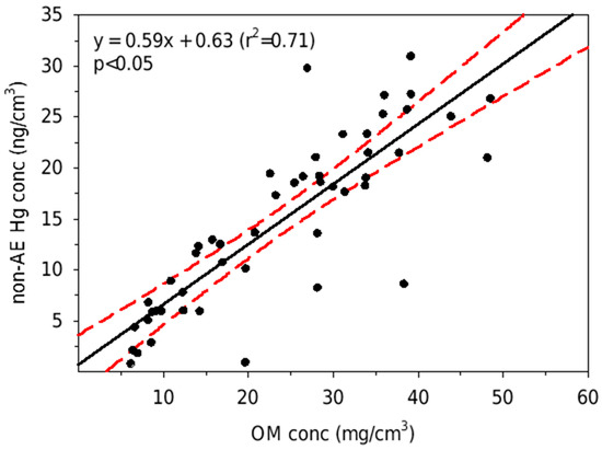
Figure 2.
The correlation between the non-AE-Hg and the OM (linear regression in the black line) with the confidence level at 95% (the red lines) in the sediments of Apalachicola Bay, North Florida, USA.
The spatial distributions of OM and total sulfides (AVS + CRS) in the sediments of the bay are presented in Figure 3. The OM was more heavily distributed in the southern area, whereas the total sulfides were more heavily distributed in the northeastern corner of the bay. The range of distribution of the total sulfides was relatively narrow in comparison to that of the OM.
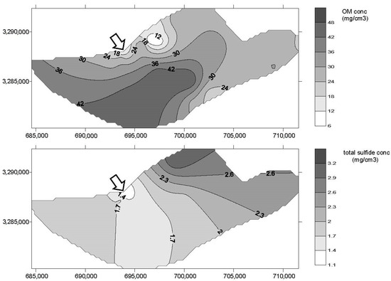
Figure 3.
The spatial distributions of the organic matter and the total sulfide (AVS + CRS) of the sediments in the Apalachicola Bay, North Florida, USA. The arrows indicate the location of the river discharge.
The spatial distribution of the Hg in the sediments of the bay is presented in Figure 4. The total Hg and sulfide-Hg were more heavily distributed in the southern area, similar to that of the OM. The potentially bioavailable non-sulfide-Hg was distributed more in the eastern and western regions, a contrasting distribution pattern from that of the total Hg or sulfide-Hg.
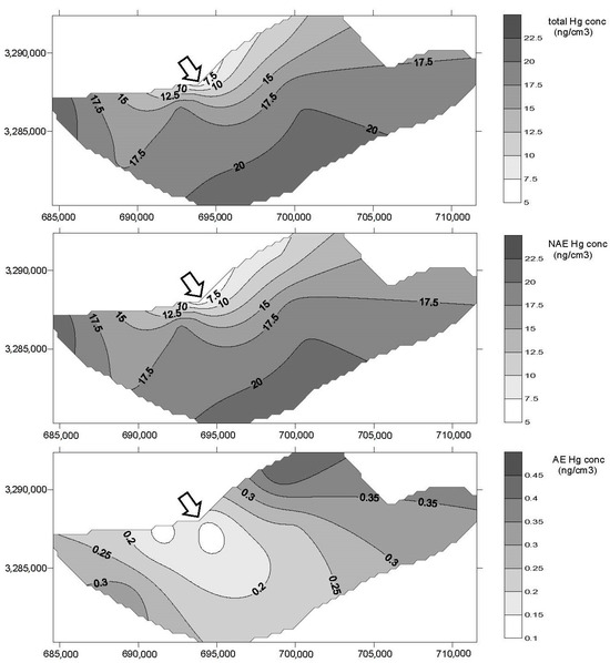
Figure 4.
The spatial distributions of the total Hg, non-AE-Hg and AE-Hg of the sediments of the Apalachicola Bay, North Florida, USA. The arrows indicate the location of the river discharge.
4. Discussion
Traditionally, all HM sulfides, including Hg sulfide, are considered to be mono-sulfides, which are AE, and inseparable from their non-sulfides analytically. Due to this limitation, methods for assessing Hg bioavailability have shifted toward operationally defined extraction and leaching methods, which are not rigorously defined [7,8,9]. A recent study has shown that Hg sulfide precipitated in sediments is not mono-sulfide but exclusively bi-sulfide, which is non-AE under nitrogen [16]. This discovery provides a chemically rigorous basis for quantifying Hg sulfide in sediments and excluding it from bioavailability assessment. The non-AE-Hg may contain Hg occluded in pyrite [28], which is also non-bioavailable. After excluding the non-AE-Hg, the AE-Hg can be considered as potentially bioavailable Hg in sediments.
The average total Hg in the sediments (13.3 ± 5.3 ng/cm3 or 31.7 ± 12.3 ng/g) was well below the average of the North American freshwater surface sediments (190 ng/g) [29]. The average potentially bioavailable Hg determined in this study (0.28 ± 0.2 ng/cm3 or 0.65 ± 0.5 ng/g) was even well below the average of the MeHg (3.83 ng/g) [29] found in the North American freshwater surface sediments. Notice that MeHg is only a fraction of the potentially bioavailable Hg.
The average Hg concentration of conterminous USA surface soils has been reported to be between 0.36 and 0.43 ng/g [30,31]. If the average Hg concentration of the North American freshwater surface sediments was 190 ng/g, the Hg concentration factor in the freshwater sediments over that of the average watershed soils was 442 to 528 times. In comparison, the Hg concentration factor in the Apalachicola Bay sediments over that of the drainage area soils, using the conterminous USA average, was only 74 to 80 times. The much lower Hg concentration factor of the Apalachicola Bay sediments compared to the national average could be attributed to either the overestimation of soil Hg in the Apalachicola River Basin or the significantly lower soil erosion rates of the river basin, which contributed to the Hg in the Apalachicola Bay. Nonetheless, the concentration factors of the aquatic sediment Hg over the terrestrial soil Hg indicate that aquatic sediments accumulate terrestrial Hg, and sulfidic sediments sequestered most (on average, >97% in this study) of the Hg into a sulfide form, which is non-bioavailable.
The sulfide content of the sediments in the bay was at least five orders of magnitude greater than that of the Hg content in the sediments. According to the solubility product constant, Hg would be the most favorable heavy metal to be sequestered as sulfide. (The solubility product constant of HgS is in the order of 10−52, compared 10−37 of CuS, and 10−22 to 10−27 of the rest of heavy metal sulfides.) [32]. This explains why Hg sulfide no longer exhibited a correlation with the total sulfides because almost all of them were already sequestered as sulfide in the sediments. The sulfide-Hg of this study was significantly correlated with the OM of the sediments (Figure 2). The spatial distribution of OM (Figure 3) in the bay was influenced by the input of the Apalachicola River, which tends to deposit fine particles and OM in the southern part bordering the barrier island [19,20]. The river flow influences the distribution of OM, which in turn influences the distribution of the total Hg and sulfide-Hg in the sediments.
The influence of dissolved organic matter (DOM) in sediment porewater may interfere with Hg sulfide formation, as suggested by a few studies [33,34,35]. DOM, especially thiol DOM, was found to reduce the MeHg bioavailability in sediments [36]. These findings, however, do not affect the conclusions of this study in assessing the potentially bioavailable Hg in aquatic systems.
Hg sulfide can only form and remain stable in certain anoxic conditions. Factors that alter the redox potential of sediments, such as dredging or disturbance (by storms or hurricanes), may lead to a change in the status and bioavailability of Hg. These changes in Hg bioavailable status in sediments, however, can be readily detected by the method proposed in this study.
5. Conclusions
Assessing bioavailable mercury in aquatic sediments is critically important to public health and ecological concerns. Currently, assessing mercury bioavailability in aquatic sediments has relied on operationally defined methods, which are not rigorous. This study presents a simple yet chemically rigorous method for quantifying Hg sulfide in sediments, which can then be excluded from the bioavailability assessment. We showed that most (on average, 97.1%) mercury has been sequestered in the sulfidic sediments of Apalachicola Bay, Florida, USA, as sulfide. The levels of the total or the potentially bioavailable mercury in the sediments were low compared to the national average. This study demonstrated that aquatic sediments accumulate mercury from terrestrial soils carried by rivers, and sulfidic sediments sequester most of the mercury into a non-bioavailable sulfide form. Mercury sulfide can form and remain stable under certain anoxic conditions of sediments. Changes in the redox potential of sediments may alter the mercury bioavailable status. The changes in mercury bioavailable status, however, can readily be detected using the method proposed in this study.
Author Contributions
Conceptualization, Y.-P.H.; methodology, Y.-P.H.; formal analysis, Y.-P.H.; investigation, Y.-P.H. and G.B.; resources, Y.-P.H.; data curation, G.B. and Y.-P.H.; writing—original draft preparation, Y.-P.H.; writing—review and editing, G.B.; supervision, Y.-P.H.; project administration, Y.-P.H.; funding acquisition, Y.-P.H. All authors have read and agreed to the published version of the manuscript.
Funding
This research was partially funded by NRI/USDA project No. 009342.
Data Availability Statement
The original contributions presented in this study are included in the article material. Further inquiries can be directed to the corresponding author.
Acknowledgments
This research was partially funded by NRI/USDA project No. 009342.
Conflicts of Interest
The authors declare no conflicts of interest.
References
- Rodrigues, P.A.; Ferrari, R.G.; Santos, L.N.; Conte, C.A. Mercury in aquatic fauna contamination: A systematic review on its dynamics and potential health risks. J. Environ. Sci. 2019, 84, 2015–2018. [Google Scholar] [CrossRef]
- Rice, K.M.; Walker, E.M.; Wu, M.; Gillete, C.; Blough, E.R. Environmental mercury and its toxic effects. J. Prev. Med. Public Health 2014, 47, 74–83. [Google Scholar] [CrossRef]
- Kwasigroch, U.; Bełdowska, M.; Jędruch, A.; Lukawska-Matuszewska, K. Distribution and bioavailability of mercury in the surface sediments of the Baltic Sea. Environ. Sci. Pollut. Res. 2021, 28, 35690–35708. [Google Scholar] [CrossRef]
- Bloom, N.S. On the chemical form mercury in edible fish and marine invertebrate tissue. Can. J. Fish. Aquat. Sci. 1992, 49, 1010–1017. [Google Scholar] [CrossRef]
- Francesconi, K.A.; Lenanton, R.C.J. Mercury contamination in semi-enclosed marine embayment: Organic and inorganic mercury content of biota, and factors influencing mercury level in fish. Mar. Environ. Res. 1992, 33, 189–212. [Google Scholar] [CrossRef]
- Benoit, J.M.; Gilmour, C.C.; Mason, R.P.; Heyes, A. Sulfide controls on mercury speciation and bioavailability to methylating bacteria in sediment pore waters. Environ. Sci. Technol. 1999, 33, 951–957. [Google Scholar] [CrossRef]
- Wallschläger, D.; Desai, M.V.M.; Spengler, M.; Wilken, R.D. Mercury Speciation in Floodplain Soils and Sediments along a Contaminated River Transect. J. Environ. Qual. 1998, 27, 1034–1044. [Google Scholar] [CrossRef]
- Beldowski, J.; Pempkowiak, J. Horizontal and vertical variabilities of mercury concentration and speciation in sediments of the Gdansk Basin, Southern Baltic Sea. Chemosphere 2003, 52, 645–654. [Google Scholar] [CrossRef]
- Sladeka, C.; Gustin, M.S. Evaluation of sequential and selective extraction methods for determination of mercury speciation and mobility in mine waste. Appl. Geochem. 2003, 18, 567–576. [Google Scholar] [CrossRef]
- Di Toro, D.M.; Mahony, J.D.; Hansen, D.J.; Scott, K.J.; Hicks, M.B.; Mayr, S.M.; Redmond, M.S. Toxicity of cadmium in sediments: The role of acid volatile sulfide. Environ. Sci. Technol. 1990, 9, 1487–1502. [Google Scholar] [CrossRef]
- Di Toro, D.M.; Mahony, J.D.; Hansen, D.J.; Scott, K.J.; Carlson, A.R.; Ankley, G.T. Acid volatile sulfide predicts the acute toxicity of cadmium and nickel in sediments. Environ. Sci. Technol. 1992, 26, 96–101. [Google Scholar] [CrossRef]
- Casas, A.M.; Crecelius, E.A. Relationship between acid volatile sulfide and the toxicity of zinc, lead, and copper in marine sediments. Environ. Toxicol. Chem. 1994, 13, 529–536. [Google Scholar] [CrossRef]
- Morse, J.W. Interactions of trace metals with authigenic sulfide minerals: Implications for their bioavailability. Mar. Chem. 1994, 46, 187–199. [Google Scholar] [CrossRef]
- Berry, W.J.; Hansen, D.J.; Mahony, J.D.; Robson, D.L.; Di Toro, D.M.; Shipley, B.P.; Rogers, B.; Corbin, J.M.; Boothman, W.S. Predicting the toxicity of metal-spiked laboratory sediments using acid-volatile sulfide and interstitial water concentrations. Environ. Toxicol. Chem. 1996, 15, 2067–2079. [Google Scholar] [CrossRef]
- Hansen, D.J.; Berry, W.J.; Mahony, J.D.; Boothman, W.S.; Di Toro, D.M.; Robson, D.L.; Ankley, G.T.; Ma, D.; Yan, Q.; Pesch, C.E. Predicting the toxicity of metal-contaminated field sediments using interstitial concentration of metals and acid-volatile sulfide normalizations. Environ. Toxicol. Chem. 1996, 15, 2080–2094. [Google Scholar] [CrossRef]
- Hsieh, Y.P. The chemical nature of mercury and copper sulfides and its implication for bioavailability assessment in sediments. Water 2024, 16, 70. [Google Scholar] [CrossRef]
- Liu, X.; Huang, W. Modeling sediment resuspension and transport induced by storm wind in Apalachicola Bay, USA. Environ. Modell. Softw. 2009, 24, 1302–1313. [Google Scholar] [CrossRef]
- Joshi, I.D.; D’Sa, E.J.; Osburn, C.L.; Bianchi, T.S.; Ko, D.S.; Oviedo-Vargas, D.; Arellano, A.R.; Ward, N.D. Assessing chromophoric dissolved organic matter (CDOM) distribution, stocks, and fluxes in Apalachicola Bay using combined field, VIIRS ocean color, and model observations. Remote Sens. Environ. 2017, 191, 359–372. [Google Scholar] [CrossRef]
- Hallas, M.K.; Huettel, M. Bar-built estuary as a buffer for riverine silicate discharge to the coastal ocean. Cont. Shelf Res. 2013, 55, 76–85. [Google Scholar] [CrossRef]
- Chen, S.; Huang, W.; Chen, W.; Chen, X. An enhanced MODIS remote sensing model for detecting rainfall effects on sediment plume in the coastal waters of Apalachicola Bay. Mar. Environ. Res. 2011, 72, 265–272. [Google Scholar] [CrossRef]
- Huang, W.; Sun, H.; Nnaji, S.; Jones, W.K. Hydrodynamics in a multiple-inlet. J. Coast. Res. 2002, 18, 674–684. [Google Scholar]
- Northwest Florida Water Management District. Apalachicola River and Bay Surface Water Improvement and Management (SWIM) Plan; Northwest Florida Water Management District: Midway, FL, USA, 2017; 137p.
- Hsieh, Y.P.; Yang, C.H. Diffusion methods for the determination of reduced sulfur species in sediments. Limnol. Oceanogr. 1989, 34, 1126–1131. [Google Scholar] [CrossRef]
- Hsieh, Y.P.; Shieh, Y.N. Analysis of reduced inorganic sulfur by diffusion methods: Improved apparatus and evaluation for sulfur isotopic studies. Chem. Geol. 1997, 137, 255–261. [Google Scholar] [CrossRef]
- American Public Health Association (APHA). Standard Methods for the Examination of Water and Wastewater, 14th ed.; American Public Health Association: Washington, DC, USA, 1976; p. 1193. [Google Scholar]
- SAS Institute, Inc. SAS User’s Guide: Statistics, Version 9; SAS Institute: Cary, NC, USA, 2005. [Google Scholar]
- Golden Software Inc. Surface Mapping System, Version 8.05; Golden Software, Inc.: Golden, CO, USA, 2004. [Google Scholar]
- Huerta-Diaz, M.A.; Morse, J.W. A quantitative method for determination of trace metal concentration in sedimentary pyrite. Mar. Chem. 1990, 29, 119–144. [Google Scholar] [CrossRef]
- Kamman, N.C.; Chalmers, A.; Clair, A.T.; Major, A.; Moore, R.B.; Norton, S.A.; Shanley, J.B. Factors Influencing Mercury in Freshwater Surface Sediments of Northeastern North America. Ecotoxicology 2005, 14, 101–111. [Google Scholar] [CrossRef]
- Andren, A.W.; Nriagu, J.O. The global cycle of mercury. In Topics in Environmental Health; The Biogeochemistry of Mercury in the Environment; Nriagu, J.O., Ed.; Elsevier/North-Holland Biomedical Press: Amsterdam, The Netherlands, 1979; Volume 3, pp. 1–21. [Google Scholar]
- Shacklette, H.T.; Boerngen, J.G. Element concentrations in soils and other surficial materials of the conterminous United States. In U.S. Geological Survey Professional Paper 1270; U.S. Geological Survey: Alexandria, VA, USA, 1984; 105p. [Google Scholar]
- Stumm, W.; Morgan, J.J. Aquatic Chemistry, 2nd ed.; John Wiley and Sons: New York, NY, USA; Chichester, UK; Brisbane, Australia; Toronto, ON, Canada; Singapore, 1981; 780p. [Google Scholar]
- Ravichandran, M.; Aiken, G.R.; Reddy, M.M.; Ryan, J.N. Enhanced dissolution of cinnabar (mercuric sulfide) by dissolved organic matter isolated from the Florida Everglades. Environ. Sci. Technol. 1998, 32, 3305–3311. [Google Scholar] [CrossRef]
- Ravichandran, M.; Aiken, G.R.; Ryan, J.N.; Reddy, M.M. Inhibition of precipitation and aggregation of metacinnabar (mercury sulfide) by dissolved organic matter isolated from the Florida Everglades. Environ. Sci. Technol. 1999, 33, 1418–1423. [Google Scholar] [CrossRef]
- Ravichandran, M. Interactions between mercury and dissolved organic matter—A review. Chemosphere 2004, 55, 319–331. [Google Scholar] [CrossRef]
- Seelen, E.; Robert Mason, R.; Liem-Nguyen, V.; Wünsch, U.; Skyllberg, U.; Baumann, Z.; Björn, E. Dissolved organic matter thiol concentrations determine methylmercury bioavailability across the terrestrial-marine aquatic continuum. Nat. Commun. 2023, 14, 6728. [Google Scholar] [CrossRef] [PubMed]


Disclaimer/Publisher’s Note: The statements, opinions and data contained in all publications are solely those of the individual author(s) and contributor(s) and not of MDPI and/or the editor(s). MDPI and/or the editor(s) disclaim responsibility for any injury to people or property resulting from any ideas, methods, instructions or products referred to in the content. |
© 2025 by the authors. Licensee MDPI, Basel, Switzerland. This article is an open access article distributed under the terms and conditions of the Creative Commons Attribution (CC BY) license (https://creativecommons.org/licenses/by/4.0/).