Abstract
In dam operations, sudden discharges during extreme rainfall events can pose severe flood risks to downstream communities. This study developed a dam discharge-based river water level forecasting model using a data-driven deep learning approach, long short-term memory (LSTM). To enhance predictive performance, physics-based HEC-RAS simulation outputs, including extreme events, were incorporated as additional inputs. The Seomjin River Basin in South Korea, which recently experienced severe flooding, was selected as the study area. Hydrological data from 2010 to 2023 were utilized, with 2023 reserved for model testing. Forecasts were generated for four lead times (3, 6, 12, and 24 h), consistent with the operational flood forecasting system of the Ministry of Environment, South Korea. Using only observed data, the model achieved high accuracy at upstream sites, such as Imsil-gun (Iljung-ri, R2 = 0.92, RMSE = 0.27 m) and Gokseong (Geumgok Bridge, R2 = 0.91, RMSE = 0.35 m), for a 6-h lead time. However, performance was lower at Gurye-gun (Songjeong-ri, R2 = 0.72, RMSE = 1.48 m) due to the complex influence of two dams. Incorporating enhanced inputs significantly improved predictions at Gurye-gun (R2 = 0.91, RMSE = 1.17 m at 3 h). Overall, models using only observed data performed better at upstream sites, while enhanced inputs were more effective in downstream or multi-dam regions. The 6-h lead time yielded the highest overall accuracy, highlighting the potential of this approach to improve real-time dam operations and flood risk management.
1. Introduction
Dams play a critical role in water resource management, hydroelectric power generation, and flood control []. However, the sudden release of water from dams during heavy rainfall, whether planned or accidental, can lead to significant downstream flooding, causing extensive damage to property, infrastructure, and riverine ecosystems. Predicting the arrival times of dam discharges is therefore a critical aspect of hydrological modeling and water resource management, particularly in regions that are prone to flooding. Accurate predictions can significantly mitigate the adverse impacts of sudden water released from dams, helping to prevent devastating downstream floods.
Few cases have focused on the flood damage caused by dam discharges within international research. For instance, in India, the Hirakud Dam in Odisha has repeatedly caused downstream flooding events (2011, 2019) due to inadequate flood forecasting and sudden emergency releases, despite the absence of structural deficiencies []. Similarly, in Nepal, mismanagement of the Kosi River barrage during the 2008 monsoon season led to massive uncontrolled releases, which triggered catastrophic flooding in the state of Bihar, northern India, that displaced millions of people []. These cases demonstrate that even without structural failures, insufficient operational planning and flood preparedness can result in large-scale disasters. In addition, during Hurricane Harvey in 2017, the U.S. Army Corps of Engineers conducted controlled releases from the Addicks and Barker Reservoirs in Houston to prevent dam overtopping or failure. However, these releases caused extensive downstream flooding along Buffalo Bayou, highlighting the complex challenges of flood management during extreme rainfall events [].
In July 2017, South Korea experienced extremely heavy rainfall, leading to significant increases in the water levels at the Daecheong Dam. To prevent overtopping, the dam operators released large quantities of water. Downstream regions, including Cheongju city and Sejong city, were severely affected. The sudden surge overwhelmed drainage systems, inundated residential and agricultural areas, and required emergency responses from local authorities. During the severe monsoon season of August 2020, the Hapcheon Dam faced rapidly rising water levels because of persistent rainfall. To prevent overtopping, emergency releases were conducted, but downstream regions such as Hapcheon County and Changnyeong County, which were already saturated by prior rains, experienced extensive flooding. Homes, farmland, and infrastructure sustained severe damage, and numerous residents were forced to evacuate. Similarly, the Seomjin River basin was critically impacted when the Seomjin River Dam, which is located upstream, was forced to release large volumes of water to prevent overtopping. With river levels already elevated due to record-breaking rainfall, the additional discharge triggered catastrophic flooding downstream, devastating the communities and agricultural lands in the Jeolla and Gyeongsang regions. These incidents highlight the urgent need for advanced technologies that can proactively forecast the downstream flood risks associated with dam releases and operations []. The Seomjin River Basin in South Korea exhibits distinct geomorphological vulnerabilities compared to other major river basins. Its steep mountainous terrain and limited flood control capacity of major reservoirs (Seomjingang Dam and Juam Dam) accelerate runoff and restrict operational flexibility during extreme rainfall events []. Unlike the Han River Basin, where extensive floodplains and large multipurpose dams (e.g., Soyang Dam) mitigate flood risks, the Seomjin Basin is characterized by narrow river reaches and simultaneous influences from multiple dam discharges, which amplify downstream flood hazards []. While the Geum River and Yeongsan River basins have larger floodplain storage and gentler slopes, the Seomjin River Basin demonstrates a higher sensitivity to dam-release-induced flooding due to its geomorphic constraints and hydrological concentration effects [].
Based on these cases, flood forecasting technologies have traditionally relied on physically based hydrological and hydraulic models, which are primarily aimed at preventing flood damage caused by rainfall-induced events. While the traditional hydrological models are effective, they often struggle with the complexity and nonlinearity that are inherent in hydrological systems. Moreover, these models typically require extensive data and complex calibration processes, making them less practical for real-time applications []. However, in cases of short-duration, high-intensity rainfall and sudden large-scale dam releases, flood prediction technologies must be adopted and validated through alternative approaches beyond the traditional methods. To address this issue, developing technologies that can accurately and rapidly predict river water levels resulting from dam releases during flood conditions is essential. In recent years, both model-based and AI-based prediction techniques have been increasingly applied to meet this need [].
Recent advances in deep learning have led to the application of various neural network architectures in hydrological forecasting scenarios. In addition to long short-term memory (LSTM) networks, models such as convolutional neural networks (CNNs), gated recurrent units (GRUs), multilayer perceptrons (MLPs), and hybrid architectures have been explored to achieve increased predictive accuracy and capture spatiotemporal dynamics in hydrological systems. For example, CNNs have been employed to extract spatial features from precipitation and land use data, which are then fed into LSTM layers for streamflow prediction, forming effective CNN–LSTM hybrids []. GRUs, which are simplified variants of LSTM, have demonstrated comparable or even superior performance to that of the existing methods in daily discharge forecasting tasks, especially in terms of computational efficiency []. Furthermore, attention-based models such as the transformer have been recently introduced to hydrology for capturing long-range dependencies in rainfall-runoff relationships, showing potential for medium-range flood forecasting [].
Despite these innovations, LSTM remains one of the most widely adopted models because of its proven ability to handle both short- and long-term temporal dependencies in time series data. According to various comparative studies, long short-term memory (LSTM) models generally exhibit superior performance to that of traditional machine learning techniques (e.g., linear regression, support vector machines, and random forests) and often outperform other deep learning models (e.g., MLPs and GRUs) in streamflow forecasting tasks [,]. Their strength is particularly evident when modeling long-term dependencies and nonlinear relationships in rainfall–runoff processes []. This study builds upon these foundations and applies LSTM-based modeling to the Seomjin River Basin to forecast dam discharge arrival times and water levels under various hydrometeorological scenarios.
Among these approaches, recent advancements in machine learning, particularly the development of long short-term memory (LSTM) networks, have shown great promise. LSTM, which is a type of recurrent neural network (RNN), is specifically designed to handle sequential data and can effectively capture both short-term and long-term dependencies within time series data. This makes LSTM particularly well suited for modeling the temporal dynamics of river discharges and predicting dam discharge arrival times []. Several studies have demonstrated the efficacy of LSTM models in hydrological forecasting scenarios. For example, research conducted on the East Branch of the Delaware River highlighted the superior performance of LSTM in terms of predicting river discharges relative to the traditional modeling approaches. The study utilized over 80 years of discharge data, demonstrating the ability of their model to handle large datasets and complex temporal data []. Similarly, in the Da River basin in Vietnam, LSTM models have achieved high accuracy with respect to predicting daily discharges, with Nash–Sutcliffe efficiency values exceeding 0.95 in some cases []. In South Korea, recent studies have also demonstrated the effectiveness of LSTM for predicting dam discharges and river flows. For example, an LSTM model was applied to predict the discharge from the Soyang River Dam, where it outperformed traditional machine learning models such as decision trees and random forests, achieving high predictive accuracy [,].
These results underline the potential of LSTM as a robust tool for dam discharge prediction, which is critical for managing downstream water levels and mitigating flood risks. Considering the diversity of hydrological and river conditions, as well as the urgent response times required for dam operations, it is imperative to develop AI-based flood forecasting technologies that ensure both accurate and rapid decision-making capabilities.
The predictive structure of the baseline LSTM algorithm in this study was adapted from the method proposed in the literature [,] and applied to the target region of interest. Recent studies have demonstrated that the use of synthetic hydrological data—generated or gap-filled by simulation models, such as HEC-RAS—can enhance the performance of machine learning models. For instance, Sergio et al. [] showed that blending synthetic and observed data yields more accurate and robust LSTM predictions than relying on either source alone. Building on this evidence, the present study investigates whether, in situations where observed dam release or downstream water level records are unavailable, incorporating synthetic HEC-RAS scenarios into LSTM training can improve predictive skill. Nonetheless, it is important to acknowledge that the effectiveness of this approach depends on the ability of physical models like HEC-RAS to adequately reproduce real-world hydrodynamics. If these models introduce systematic biases, their outputs may mislead the LSTM and potentially degrade predictive performance.
2. Materials and Methods
The ultimate goal is to advance the model to a practical level, enabling the prediction of river water levels and arrival times of dam discharges. This study aimed to predict the water level caused by dam discharges at major monitoring stations along the Seomjin River Basin in South Korea. Specifically, LSTM algorithms were developed for lead times of 3, 6, 12, and 24 h to forecast the river water levels associated with dam discharges by utilizing a variety of hydrometeorological datasets. Furthermore, input data optimization and enhanced input variables, including hybrid model data within an AI system, were conducted to evaluate and enhance the achieved predictive accuracy (Figure 1).
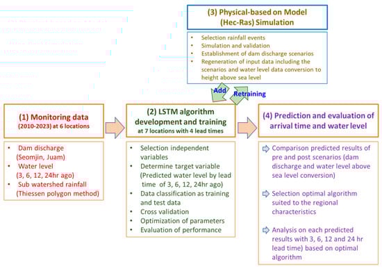
Figure 1.
The process of constructing the LSTM algorithm for generating enhanced data from the HEC-RAS model.
In addition, this study serves as a preliminary evaluation aimed at establishing guidelines for the practical adoption of AI-based flood forecasting in the operational framework of the Korean Ministry of Environment’s Flood Control Office. The primary focus lies in post-modeling analysis of results to maximize predictive performance for flood forecasting. In operational practice, the existing system automatically collects and processes all hydrological data, including dam releases and river water levels, through real-time quality control. These processed datasets are then directly used within the LSTM-based real-time river stage forecasting system. Consequently, the configuration of input data in practice is predefined to ensure compatibility with the operational system, while uncertainties in the datasets are minimized through automated quality assurance. The emphasis of this research, therefore, is on developing methods to optimize site-specific input datasets in order to further enhance forecasting performance.
2.1. Study Area in the Seomjin River Basin
The Seomjin River basin contains two multipurpose dams: Seomjin River Dam (SRD) and the Juam Main Dam (JMD). Additionally, outside the basin, the Juam Regulating Dam; water supply dams such as Dongbok Dam and Donghwa Dam; and a hydroelectric dam, the Boseong River Dam, are present. The total effective storage capacity of the Seomjin River Dam and Juam Main Dam is 781 million m3, of which approximately 90 million m3 is utilized as flood control capacity, playing a crucial role in preventing flood damage in the Seomjin River basin. The key specifications of the SRD and JMD and their basin characteristics are shown in Table 1 and Figure 2b, with designed flood discharge rates for spillway releases of 1868 m3/s and 4154 m3/s, respectively.

Table 1.
Dam release cases under rainfall events in this study.
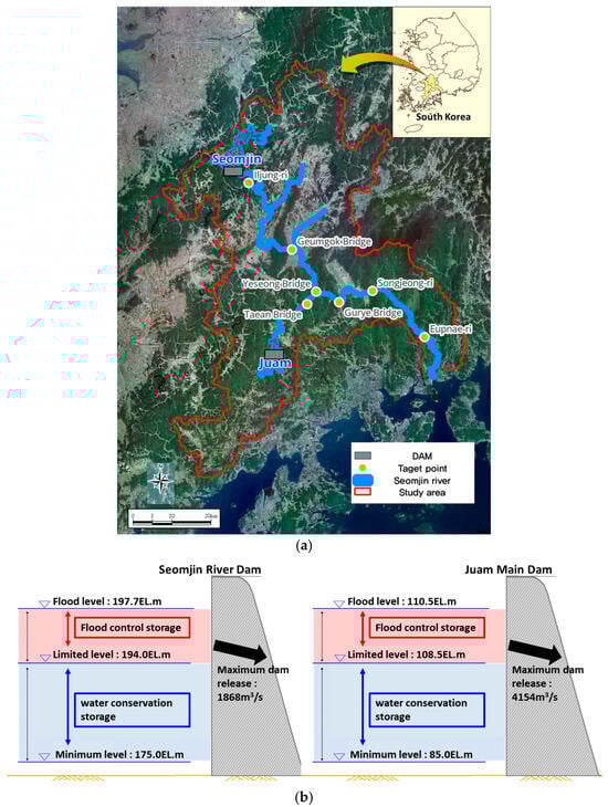
Figure 2.
Target points of this study in the Seomjin River Basin: (a) locations of the water level stations in the study area; (b) maximum dam release points (for the SRD and JMD).
The input data required for this study consisted of three main categories: precipitation, dam inflow/outflow, and river water levels. Precipitation data at 10-min intervals were obtained from the Korea Meteorological Administration (KMA) Open Data Portal (https://data.kma.go.kr). Dam inflow and outflow records, also at 10-min intervals, were collected from the Korea Water Resources Corporation’s MyWater portal (https://www.water.or.kr). In addition, river water level data were acquired from the Yeongsan River Flood Control Office (https://www.yeongsanriver.go.kr) with a frequency of 10 min. All datasets were compiled and processed to construct the input variables for model development.
Over the past 20 years (2000–2019), the average annual total utilization of major dams (Water Resources Management Information System, http://www.wamis.go.kr) was 2086.2 million m3. The total water use was distributed as follows: 692.2 million m3 (33.18%) for municipal and industrial purposes, 600.5 million m3 (28.79%) for agricultural purposes, and 38.5 million m3 (1.85%) for river maintenance. Moreover, 754.9 million m3 (36.19%) was discharged through overflow and spillways. For the SRD, the largest portion of the total usage of 543.3 million m3 was for agricultural water, amounting to 470.9 million m3 (86.7%). For the JMD, the largest portion of the total usage of 373.1 million m3 was for municipal and industrial water, at 195.8 million m3 (52.5%).
In this study, a total of seven water level observation stations within the Seomjin River basin were affected by dam discharges. These include sites influenced by the SRD, such as Imsil-gun (Iljung-ri), Gokseong-gun (Geumgok Bridge), and Gokseong-gun (Yesung Bridge). Additionally, Gokseong-gun (Taean Bridge) on the Boseong River was influenced by the JMD, and the sites influenced by both dams included Gurye-gun (Gurye Bridge), Gurye-gun (Songjeong-ri), and Hadong-gun (Eumnae-ri), as shown in Figure 2a.
2.2. Theory of the Long Short-Term Memory (LSTM) Algorithm
Deep learning can extract or represent the complex and nonlinear characteristics of natural systems to produce corrected and predictive information, and it is currently being actively researched in various fields. Accordingly, deep learning technology can also be utilized as an effective and feasible option in the field of water resources. According to previous work [], the construction of large-scale observation networks has made data collection easier than in previous generations, and the rapid development of computing resources is expected to lead to the application of a wider range of deep learning technologies in water resource management and disaster response scenarios. In particular, LSTM is widely used for time series forecasting, particularly for streamflow and flood prediction. Approximately 35–40% of hydrology studies leverage LSTM networks, reflecting their strength in capturing temporal dependencies [].
The LSTM algorithm was developed to address the vanishing gradient problem faced by recurrent neural networks (RNNs). It consists of a forgetting gate (Equation (1)), an input gate (Equation (2)), a cell state (Equations (3) and (4)), and an output gate (Equations (5) and (6)). The main difference between an RNN and an LSTM network is the introduction of a cell state, which updates the state value at a specific time point. This allows the model to decide whether to update the information stored internally, enabling it to effectively utilize past time series data. Owing to this ability to remember more data variations over time, LSTM networks are efficient at capturing long-term temporal dependencies, making them well suited for various time series learning tasks. LSTM networks have been widely applied not only in speech recognition, language modeling, and translation but also in other fields in combination with other neural networks [].
Here, represents the sigmoid activation function; tanh represents the hyperbolic tangent activation function; ,,, and represent the weights of different gates; ,,, and represent the biases of the different gates; represents the previous cell state; represents the candidate cell state; and represents the cell state at the current time point.
2.3. Theory of the HEC-RAS Model
HEC-RAS has been widely applied in previous studies [,] to reproduce water level dynamics under conditions where observations are limited or unavailable, particularly during extreme events, such as floods or high dam releases. These studies have demonstrated that simulated outputs from HEC-RAS can be effectively combined with LSTM or other deep learning-based forecasting models to improve predictive performance. Building on this evidence, the present study employed HEC-RAS to generate simulated river water level datasets corresponding to unmonitored dam release scenarios.
River water levels must be calculated using appropriate methods, such as steady-flow, gradually varying-flow, or unsteady-flow computations, on the basis of the observed flow conditions. In long, uniform channels where the cross-sectional shapes and slopes are constant, a steady flow is achieved when a constant discharge occurs, causing the depth and velocity of the water to become uniform across all sections. However, in natural rivers, the cross-sectional shapes are irregular, meaning that, in a strict sense, steady flows do not exist in natural rivers. When the cross-sectional shape, slope, and friction of a channel vary, the flow deviates from a steady state and becomes a gradually varying flow (GVF). The influence of the GVF causes the water surface profile to pull or push the steady flow upstream or downstream (depending on the flow conditions), and this influence propagates both upstream and downstream. In this study, for water level estimation purposes, the unsteady flow method was adopted while utilizing HEC-RAS (the Hydrologic Engineering Center (HEC) developed the River Analysis System) model developed by the U.S. Army Corps of Engineers (USACE). The modeling framework is based on unsteady-flow simulations using the HEC-RAS model. The unsteady-flow computation in HEC-RAS solves the full one-dimensional Saint-Venant equations of continuity and momentum to represent time-dependent variations in discharge and water surface elevation. This method enables the model to capture transient flow conditions, such as rapid changes in river stage due to dam releases, flood wave propagation, and channel storage effects. By applying this approach, the temporal dynamics of river levels can be more accurately reproduced, thereby providing a realistic basis for evaluating downstream water level responses under various dam operation scenarios.
For ungauged locations, the HEC-RAS model was constructed and validated using data acquired from the river master plan to build input data for the estimation model. In this study, HEC-RAS was used for locations without observed data, and 10-min interval data were generated.
The basic equations of the HEC-RAS model are dynamic equations used for 1-dimensional unsteady flow analyses in natural rivers; they include a continuity equation and a momentum equation. The continuity equation represents the principle of mass conservation within the system and is expressed as Equation (7) [].
where represents the distance along the channel, t denotes time, is the discharge, refers to the cross-sectional area, is the storage volume, and is the lateral inflow per unit length. This equation can be expressed separately for the main channel and the floodplain, as shown in Equation (8) and Equation (9), respectively.
The terms c and f refer to the main channel and the floodplain, respectively. represents the lateral inflow per unit length into the floodplain, whereas and indicate the exchange of water between the main channel and the floodplain. This equation approximates the implicit finite-difference method, and the momentum equation is based on the principle that the observed change in momentum is equal to the external forces acting on the system. The equation for a single channel can be expressed as follows.
In this context, represents gravitational acceleration, denotes the friction slope, and indicates the flow velocity. The final form of the momentum equation, which is defined using the unit-length momentum flux, flow path, and friction slope, is expressed as follows.
2.4. Dam Release Data and Design of LSTM Algorithm
To simulate and predict the downstream river water level rise caused by dam discharges over time, constructing input data for each event in which actual dam releases occurred and rainfall events took place within the watershed is necessary. Therefore, in this study, actual cases from 2010 to 2023, where dam discharges and rainfall events in the watershed caused increased downstream river water levels, were selected as rainfall events for constructing the input data, as shown in Table 1. In particular, the data from 2023 were excluded from learning as the hold-out test period in order to incorporate synthetic HEC-RAS scenarios into LSTM training data.
2.4.1. Dam Release Input Data with Additional Scenarios Involving the SRD and JMD for Simulating HEC-RAS
In cases with insufficient observational data or the failure to consider extreme values such as the maximum dam release or rainfall values, capturing the maximum water level during model training can be difficult. This makes it challenging to reflect a wide range of hydrological events and can pose problems when predicting extreme hydrological events in the future. This study generated extreme hydrological events using a physical model and combined both observational data and simulated data. By creating a synthetic hydrological dataset (observed data + scenario data), we conducted training and prediction. Based on the mean dam release events observed in the past, hypothetical scenarios were generated by proportionally increasing or decreasing the maximum dam release, thereby reconstructing unobserved release events without records of peak or actual releases, as illustrated in Figure 3. These scenarios were simulated using HEC-RAS to produce input data for the LSTM model. Furthermore, to reduce the uncertainty in the integrated dataset, calibration and validation of the HEC-RAS model were conducted.
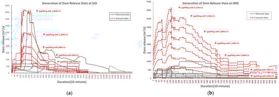
Figure 3.
Synthetic hydrological dataset of dam release with observed and scenario data: (a) SJD and (b) JMD.
Before creating the hybrid dataset, we based it on actual dam release records from the SRD and JMD. Because dam releases are strictly limited by rainfall, dam operations, and downstream river conditions, the number of observed events involving downstream river level increases caused by dam releases was also limited. Therefore, we included real rainfall events that triggered dam releases at the SRD and JMD and added dam release scenarios ranging from the minimum designed release to the maximum release at regular intervals. Ultimately, we fused the observational data with downstream river water levels simulated using HEC-RAS to create a synthetic hydrological dataset, as shown in Table 2, which was then used to regenerate the LSTM training data.
Table 2.
Maximum dam release at each downstream observation station affected by each dam release and additional scenarios at the SRD and JMD.
2.4.2. LSTM Structure in This Study
To optimize the LSTM algorithm, the structure of the LSTM was as follows: (1) data splitting (training and test), (2) K-fold cross-validation, (3) optimal parameter tuning using grid search, and (4) result prediction. In deep learning, two tasks are commonly performed at the same time in data pipelines: cross-validation and (hyper)parameter tuning. Cross-validation is the process of training learners on one set of data and testing them on a different set. Parameter tuning is the process of selecting the parameter values that maximize the accuracy of the examined model. For cross-validation, k-fold cross-validation was used as a training method. The k-fold cross-validation separated the training data into “k” folds without overlap. One set of k folds was separated via training and validation. Hence, k models were constructed, and the models were trained k times. To reduce variability, multiple rounds of cross-validation were performed using different partitions, and the results were averaged over the rounds to estimate a final predictive model. In the next step for optimizing the parameters, the grid search library exhaustively considered all the parameter combinations for the optimal parameters. The library implemented a “fitting” method and a “prediction” method, such as any classification or regression approach, except that the parameters used for prediction were optimized by cross-validation. The grid search library consisted of an estimator (a regressor or classifier), a parameter space, a method for searching or sampling candidates, a cross-validation scheme, and a score function. When the grid search library was called to fit data, it selected the parameters on a specified parameter grid, maximizing a score (the score method of the underlying estimator). Prediction, scoring, and transformation were then delegated to the tuned estimator.
As foundational data for applying the LSTM model, we selected influencing factors based on their direct impacts on peak river levels caused by dam releases, as well as forecasted dam discharges and predicted rainfall in each subwatershed. To align with operational practice, the model design followed the flood forecasting standards of the Ministry of Environment, South Korea (https://www.yeongsanriver.go.kr), which employ four lead times (3, 6, 12, and 24 h). Accordingly, the input variables included (i) observed releases from the Seomjin Dam (SRD) and Juam Dam (JMD) at 3, 6, 12, and 24 h prior to the lead time; (ii) forecasted releases from both dams at the same four lead times; (iii) historical Thiessen polygon area-averaged rainfall at six upstream locations—Imsil-gun (Iljung-ri), Gokseong-gun (Geumgok Bridge), Gokseong-gun (Yesung Bridge), Gokseong-gun (Taean Bridge), Gurye-gun (Gurye Bridge), and Gurye-gun (Songjeong-ri)—for lead times of 3, 6, 12, and 24 h; and (iv) forecasted Thiessen polygon area-averaged rainfall for the same intervals. In addition, 10-min interval data of prior river levels at each gauging station (3, 6, 12, and 24 h earlier) were included as predictors. The dependent variable was defined as the river water level at the six gauging locations for 3, 6, 12, and 24 h ahead, as summarized in Table 3.
Table 3.
Input variables at observation stations affected by dams for LSTM training.
The outliers generated during the data preparation process were preprocessed by examining the temporal consistency of the data and cross-referencing them with other variables, as these outliers could introduce uncertainty to the training process and results of the model. Moreover, as indicated in Table 1, standardization of individual variables is required for model training. Therefore, we used Python 3.2 vesion’s min–max scaler to normalize the input data between 0 and 1. The collected data from 2010 to 2022, spanning 13 years, were used for model training and validation purposes, with 80% of the data designated for training and 20% for validation. The hydrological events from 2023 were then used to compare and analyze the prediction accuracy of the LSTM model. To quantify the prediction accuracy, we selected the RMSE (root mean square error) and NSE (Nash-Sutcliffe efficiency) as performance evaluation metrics for the prediction results [,].
3. Results
3.1. Evaluation of the HEC-RAS Model
For the preparation of additional scenarios that combined observed and simulated data, this study developed results representing increases in downstream river water levels under hypothetical dam discharges. Since the purpose of scenario generation was to produce extreme events exceeding the historical maximum dam discharges, the HEC-RAS model was calibrated and validated using rainfall events associated with observed dam discharges that produced peak downstream flood levels. Thus, the calibration process was carried out with recorded dam discharges and rainfall events from the SRD and JMD, selecting the longest event in terms of dam release duration. According to Moriasi et al. [], model performance can be considered satisfactory when NSE > 0.50, R2 > 0.60, RSR ≤ 0.70, and PBIAS is within ±25% for streamflow.
The validation period for the SRD was from 12 July to 23 July 2023, with a maximum dam discharge of 692.29 m3/s. The validation sites were Imsil-gun (Iljung-ri) and Gurye-gun (Gurye Bridge). For the Bosung River, validation was performed using the maximum dam discharge of 395.67 m3/s at Moksadong 1 Bridge during 9–20 August 2023. This site was additionally used only for calibrating the HEC-RAS modelling results. Because unsteady flow analysis requires lateral inflow data, observed flow records were applied to generate inflows for subcatchments. Differences between simulated and observed water levels were minimized by adjusting Manning’s roughness coefficients (Figure 4). For all three calibration and validation sites, the model performance was satisfactory, with R2 values above 0.94 and NSE values above 0.50, and the validated results were subsequently used to construct additional scenario input datasets.
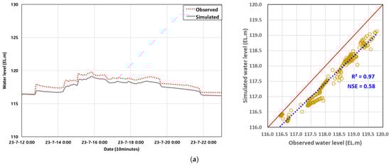
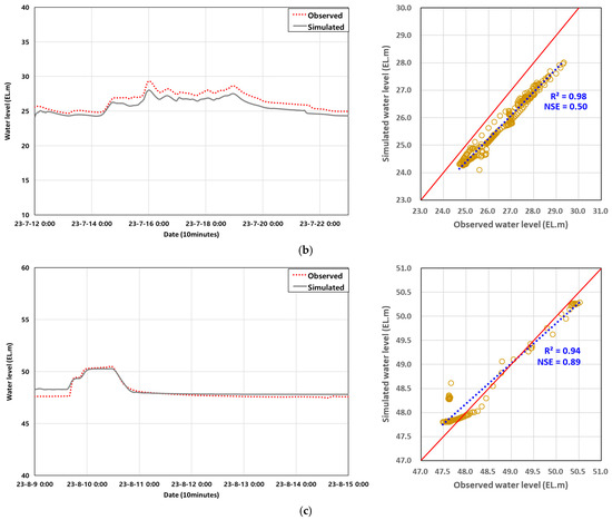
Figure 4.
Comparison between the observed and simulated water level results produced using the HEC-RAS model. The yellow circles indicate the observed and simulated water levels, the blue dotted line represents the regression (R2) trend line, and the red dotted line denotes the 1:1 reference line (R2 = 1). (a) Imsil-gun (Iljung-ri); (b) Gurye-gun (Gurye Bridge); (c) Mok-sadong-1 Bridge.
The initial Manning’s roughness coefficient for the Seomjin River, affected by the Seomjin Dam, ranged from 0.02 to 0.053. At the validation point in Imsil-gun (Iljung-ri), the roughness coefficient was adjusted to 0.032 to 0.053, resulting in an RMSE of 0.60 and an NSE of 0.58, indicating a good match with the observed water levels. For the Bosung River, influenced by the Juam Dam, the initial roughness coefficient was 0.031. At the validation point, the Moksadong 1 Bridge, the final roughness coefficient was adjusted to 0.02 to 0.049, resulting in an RMSE of 0.92 and an NSE of 0.46. Finally, for the downstream Seomjin River, which was influenced by both the Seomjin and Juam Dams, the initial roughness coefficients ranged from 0.02 to 0.053. At the validation site in Gurye-gun (Gurye Bridge), the roughness coefficient was adjusted from 0.029 to 0.058, resulting in the highest significance, with an RMSE of 0.3 and an NSE of 0.9 relative to the observed water levels.
3.2. Evaluation of LSTM Training Performance with the Original Input Data
Based on observational data, input datasets were constructed to train an LSTM algorithm, and the optimal parameters for the six target stations are summarized (see Appendix A). Despite incorporating various activation functions (sigmoid, tanh, linear, PReLU, ReLU, and softplus functions) as part of the parameter tuning process, the results for all six stations converged to either the sigmoid or linear activation functions. The performance of the model was evaluated using R2 and RMSE, as shown in Table 4. In hydrological water level–discharge prediction modeling, R2 values greater than 0.6 are generally considered acceptable, and RMSE values closer to zero indicate better performance, with values less than half the standard deviation of the observed data typically regarded as satisfactory.
Table 4.
The statistics regarding the prediction accuracy of the LSTM results produced with the optimal parameters found during LSTM training using the original input data.
The stations at Imsil-gun (Iljung-ri), Gokseong-gun (Geumgok Bridge), and Gokseong-gun (Taean Bridge) showed highly accurate water level predictions, with R2 values exceeding 0.61 and RMSE values below 0.53 m for lead times of 3, 6, and 12 h. Moreover, the predictions produced based on 24-h lead times also demonstrated statistical significance, with R2 values greater than 0.42 and RMSE values less than 0.49. However, the stations at Gurye-gun (Yesung Bridge) and Gurye-gun (Gurye Bridge) yielded unsatisfactory results for the 12-h and 24-h lead times. The Gurye-gun (Songjeong-ri) station showed poor prediction performance at all lead times (6, 12, and 24 h), indicating the limited applicability of the model for longer time horizons.
From an operational perspective, appropriate lead times for predicting water levels caused by dam releases can be summarized as follows: up to 12 h for Imsil-gun (Iljung-ri), Gokseong-gun (Geumgok Bridge), and Gokseong-gun (Taean Bridge); up to 6 h for Gurye-gun (Yesung Bridge) and Gurye-gun (Gurye Bridge); and only up to 3 h for Gurye-gun (Songjeong-ri). These differences in appropriate lead times appeared to be influenced by the upstream–midstream–downstream positions of the stations. Imsil-gun (Iljung-ri) and Gokseong-gun (Geumgok Bridge) are located in the upstream region directly downstream of the SRD, whereas Gokseong-gun (Taean Bridge) is situated in the upstream region below the JMD. In contrast, Gurye-gun (Yesung Bridge) and Gurye-gun (Gurye Bridge) are located downstream of the confluence of the Seomjin River and the Boseong River, which are influenced by releases from both the SRD and JMD, leading to increased long-term prediction difficulty owing to the complex interplay of multiple inflows. Gurye-gun (Songjeong-ri), located in the lowermost reach of the Seomjin River system (approximately 42 km upstream from the estuary), is influenced by numerous tributary inflows and storage effects, further complicating the prediction process. As a result, LSTM-based forecasts produced using past data exceeding 6 h are considered unreliable at this site because of the increased uncertainty and reduced predictability of the water levels.
3.3. Evaluation of LSTM Training Performance with the Enhanced Input Data
A previous study [] compared two models by incorporating scenario-based extreme runoff events to evaluate their prediction performance, even when such extreme events were not present in the original training dataset. Building upon the findings of this study, the present research aimed to evaluate the predictive performance of a learning algorithm that integrates results from a physical model. Furthermore, we propose an approach for optimizing the model on a site-specific basis to increase its forecasting accuracy.
The scenario data for the SRD and JMD were found to influence all six target stations, resulting in reoptimized model parameters that differed from those derived from the original dataset. After incorporating the scenario data, the optimized parameters varied across all the stations. Notably, the learning rates tended to increase, whereas the batch sizes generally decreased. This trend is presumed to reflect the adaptation of the model to the increased data complexity introduced by the scenario inputs. A higher learning rate may have facilitated faster convergence by enabling the model to adapt more rapidly to the new, more complex data patterns during the early stages of training. Conversely, the reduction in the batch size likely allowed for more detailed gradient updates per batch, making the model more sensitive to local patterns. This adjustment is interpreted as a strategy for enhancing the generalization performance of the model when it learns from diverse and complex scenario datasets (see Appendix B).
Table 5 presents a comparative analysis of the water level prediction results produced when the final LSTM model was used for six observation points within the Seomjin River Basin. Two different input data configurations were used: ❶ the original input data and ❷ the enhanced input data. The forecasting lead times were set to 3, 6, 12, and 24 h, and the performance of the model was evaluated using two metrics: the coefficient of determination (R2) and the root mean square error (RMSE).
Table 5.
The statistics of the LSTM training results produced with optimal parameters with ❶ the original input data and ❷ the enhanced input data.
First, in the observation site comparison, the original input data (❶) generally showed superior performance at the Iljung-ri, Geumgok Bridge, Yesung Bridge, Taean Bridge, and Gurye Bridge stations. In contrast, the enhanced input data (❷) performed better at the Songjeong-ri station. At Iljung-ri, the original input data consistently outperformed the enhanced data across all lead times, with the highest R2 observed for the 6-h lead time. Similarly, the Geumgok Bridge, Yesung Bridge, and Taean Bridge stations also yielded better performance with the original input, particularly at 3 or 6 h. At the Gurye Bridge station, although the differences between the R2 and RMSE values of the two input types were minor, the original input demonstrated more consistent and reliable performance. On the other hand, at the Songjeong-ri station, the enhanced input data yielded superior R2 values across all lead times, with an R2 of 0.96 at the 3-h forecast, indicating a significant improvement.
Next, an analysis of the performance trends based on the lead times revealed a general pattern where R2 decreased and the RMSE increased as the lead time increased. For most stations—Iljung-ri, Geumgok Bridge, Yesung Bridge, and Taean Bridge—the highest R2 was recorded at the 6-h lead time, with the performance decreasing at 12 h, 24 h, and 3 h (in order). For the Gurye Bridge, the highest performance was observed at 3, 6, and 12 (=24) h (in order). At Songjeong-ri, based on the enhanced input results, the performance was best at 3, 6, 24, and 12 h (in order). Across all the sites, the accuracy of the short-term forecasts (3–6 h) was relatively high.
The findings of this study suggest that data enhancement does not necessarily guarantee improved model performance; rather, the hydrological and topographic characteristics of each site, together with the suitability of the input data, play critical roles. According to Tursun et al. [], river stage prediction performance is generally influenced by terrain attributes, such as catchment area and elevation. However, for dam-release-driven river stage forecasting, as in this study, the dominant factor is the travel time required for released water to propagate from the dam to downstream observation sites. Hunt et al. [] further demonstrated that the predictive performance of LSTM models is highly sensitive to the spatiotemporal lag structure of the inputs, underscoring the importance of appropriately incorporating time delays into the model design. Consistent with these findings, our results indicate that the optimal lead time for accurate prediction varies depending on the travel time and lag associated with each monitoring site. Moreover, static physiographic attributes, such as channel length, slope, and flow path connectivity, also play a decisive role, as they determine how storage, attenuation, and transmission losses accumulate along the river corridor. In particular, as the geographic distance from the dam increases, the cumulative effects of storage, losses, and travel time become more pronounced. Therefore, the selection of an appropriate forecast horizon—such as 24 h or longer lead times—becomes essential to compensate for these factors. The Songjeong-ri case exemplifies this relationship: while the original input design performed poorly, a substantial improvement was achieved when enhanced inputs were incorporated with a 24-h lead time. This underscores the importance of preprocessing and carefully configuring input data. Furthermore, the consistently strong performance observed at the 6-h lead time suggests that this time window may serve as a practical benchmark for real-time operational decision-making in future flood forecasting applications.
4. Discussion
This study aimed to generate additional training inputs that reflect water level conditions beyond those captured in the observed datasets, thereby enabling model retraining under a broader range of dam discharge scenarios. The Seomjin River Basin, which serves as the study area, has been selected for a pilot application of Korea’s AI-based flood forecasting system. Accordingly, the primary objective of this work was to examine the predictive performance of LSTM models, identify optimal data configurations for individual monitoring sites, and explore the structural characteristics of the algorithms. These findings are intended to provide a basis for assessing the potential effectiveness of AI-based flood forecasting prior to full-scale implementation in other river basins.
It is important to note that the forecasting performance of deep learning algorithms was not evaluated using the entire dataset for training. Instead, a hold-out test period was adopted to provide an independent assessment of predictive skill. Specifically, the year 2023 was designated as the hold-out period, and model outputs were compared with observed data during this interval to evaluate generalization ability. Figure 5 presents a comparison between observed water levels and forecasts generated by two LSTM models at each monitoring site under a 6-h lead time. The blue dashed lines indicate predictions derived solely from observed data (Obs. Data prediction), whereas the red dashed lines represent forecasts obtained using the enhanced dataset that combines observed and simulated hydrological variables (Obs + Sim. Data prediction).
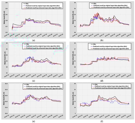
Figure 5.
Evaluation of the prediction performances achieved by two algorithms based on different input data types during the hold-out test period. (a) Imsil-gun (Iljung-ri); (b) Gokseong-gun (Geumgok Bridge); (c) Gokseong-gun (Yesung Bridge); (d) Gokseong-gun (Taean Bridge); (e) Gurye-gun (Gurye Bridge); (f) Gurye-gun (Songjeong-ri).
When the original input data were used, the performance of the model at each site yielded coefficients of determination (R2) of 0.62 (Iljuung-ri), 0.89 (Geumgok Bridge), 0.69 (Yesung Bridge), 0.89 (Taean Bridge), 0.62 (Gurye Bridge), and 0.71 (Songjeong-ri). The corresponding Nash–Sutcliffe efficiency (NSE) values were 0.50, 0.84, 0.64, 0.86, 0.60, and 0.55, respectively. On the other hand, the model using the enhanced input data yielded R2 values of 0.90 (Iljuung-ri), 0.72 (Geumgok Bridge), 0.85 (Yesung Bridge), 0.77 (Taean Bridge), 0.87 (Gurye Bridge), and 0.95 (Songjeong-ri), with corresponding NSE values of 0.46, 0.58, 0.80, 0.72, 0.87, and 0.88, respectively. These results suggest that the predictive performance of the LSTM algorithm varies depending on the input data configuration and the location of the monitoring site. Specifically, at sites located immediately downstream of major dams—namely, Iljuung-ri (Imsil County), Taean Bridge (Gokseong County), and Geumgok Bridge (Gokseong County)—the model using the original observed data outperformed the model incorporating the simulated data. This implies that in regions where dam discharges directly influence river stages, real-time observed data may better capture abrupt water level changes.
To strengthen the persuasiveness of this study, the results were compared with similar previous research. For example, Sergio et al. [] reported that when using only observed data (RERF1), prediction accuracy for high flows was limited, whereas combining observed and synthetic data (RERF2) significantly improved performance. For events with a return period greater than three years, the RMSE decreased by about 23% and the PBIAS by nearly 39%. Overall, incorporating synthetic data proved most effective in reducing the underestimation of extreme flows, thereby enhancing model robustness under high-flow conditions.
In contrast, the present study applied additional synthetic dam release scenarios for LSTM training, and the outcomes varied across sites due to differences in flood travel time from the dam. Although prediction accuracy for high flows improved at some locations, performance decreased at others, indicating the need to consider site-specific characteristics and data availability when constructing training datasets. Unlike previous studies that focused exclusively on mitigating underestimation in high-flow conditions, our results highlight that performance evaluation must also account for low- and medium-flow regimes. Nevertheless, this study confirms that incorporating synthetic data is particularly beneficial for downstream areas strongly influenced by dam releases, where improvements in high-flow prediction are most pronounced.
Conversely, at locations farther downstream or those that were influenced by combined discharges from multiple reservoirs, the model utilizing the enhanced input data demonstrated superior predictive performance. This finding indicates that incorporating simulated hydrological variables helps to represent the more complex hydrological responses in such areas. Therefore, while dam discharge is a critical factor that influences river stage forecasts, other factors, such as rainfall, the flood wave travel time, and channel storage effects, must also be considered. The selection of the most appropriate forecasting algorithm should be based on the hydrological and geomorphological characteristics of each monitoring site. In conclusion, this study recommends employing algorithms that utilize enhanced input data—combining observed and simulated variables—for regions affected by multiple dam discharges or those that are located at greater distances downstream, where various hydrological processes may act during flood routing.
In comparison with previous studies, this research demonstrates several distinctive aspects that reinforce its scientific contribution. For instance, Lee et al. [] and Hong et al. [] developed LSTM-based dam discharge prediction models within single-reservoir systems, where hydrological variability was relatively limited. While their models successfully captured temporal dependencies in flow time series, they did not fully represent the compound hydraulic interactions arising from concurrent multi-dam operations.
In contrast, the present study extends the application of data-driven techniques to complex multi-dam river systems by integrating synthetic hydrodynamic scenarios derived from HEC-RAS simulations. This integration enables the LSTM to reproduce nonlinear dynamics such as backwater effects, delayed flood waves, and reservoir coordination processes that cannot be fully characterized using observed data alone. Moreover, whereas previous works primarily emphasized high-flow conditions, the present findings demonstrate that the inclusion of simulated inputs enhances model robustness across multiple flow regimes, including medium and low flows. These improvements substantiate the synergistic potential of coupling physics-based and data-driven methods, bridging the gap between empirical data limitations and real-world hydrodynamic complexity.
Therefore, the hybrid framework proposed in this study provides a transferable and adaptive approach for AI-assisted flood forecasting, particularly in data-scarce and hydrologically complex basins.
5. Conclusions
Through the results and discussion presented in this study, we derived key implications regarding the objectives and outcomes of our research. The primary aim of this work was to evaluate how HEC-RAS scenario outputs—developed under conditions with missing observations (e.g., dam release data and downstream river stage records)—influence the predictive performance of LSTM models. By doing so, this study provides a foundational analysis toward establishing guidelines for the practical application of AI-based flood forecasting. This research further emphasizes the importance of integrating data-driven and physics-based approaches to enhance the operational reliability of flood forecasting models. In particular, the findings demonstrate that synthetic hydrodynamic scenarios can effectively supplement limited observational datasets, ensuring more comprehensive coverage of flood conditions.
The findings indicate that, for operational use, the construction of site-specific optimal input datasets should take precedence. In particular, the performance of LSTM models must be improved not by uniformly applying HEC-RAS scenario outputs, but by optimizing them according to the site-specific travel times of dam releases to downstream monitoring points. The results further reveal that prediction accuracy varies significantly across sites, underscoring the necessity of pre-operational performance evaluation, site-specific optimization, and continuous model updating through the inclusion of additional flood events. These steps are critical to ensure that the algorithm accounts for the unique physiographic characteristics of each basin. Such an approach provides a structured pathway for achieving both predictive accuracy and adaptability, allowing AI-based systems to better capture local hydrological diversity and complex dam–river interactions.
In addition, this study highlights considerations for future research and operational practice that were not addressed in detail here. Specifically, improvements to the training data consisted of two key components. First, river stage data were transformed from relative water level units (m) into absolute elevation units (EL.m). EL.m represents the absolute water level referenced to the national elevation datum, which in South Korea is defined relative to the national benchmark located 26.687 m above mean sea level at Incheon Port. Second, model-based simulation scenarios reflecting river stage increases caused by dam releases were incorporated as supplemental inputs. Previous studies [] have suggested that issues related to data shifts can be effectively mitigated by constructing input datasets based on consistent observation references. Similarly, other works [] have emphasized the importance of validating data during periods affected by altered observation standards or anomalies, highlighting that consistency and reliability in observation datasets are essential for robust model development. The integration of these procedures highlights the significance of maintaining data consistency and standardized reference levels, which form the foundation for transferable and reproducible AI applications in hydrology.
Figure 6 illustrates the river stage at the Songjeong-ri station in Gurye-gun, which was used in this study. At this location, the reference elevation (data) changed during the observation period, which altered the base water level (m). If such shifts are not corrected during the learning process, the aforementioned issues can arise. Therefore, while incorporating a wide range and volume of input time series data is valuable, ensuring the consistency of variables that reflect the same physical property is a critical step for improving the performance of models and ensuring their prediction reliability. Ultimately, this study proposes that for achieving accurate river stage forecasting under dam release scenarios, optimizing the utilized algorithm requires not only the use of consistent input data but also the consideration of site-specific river topography parameters—such as the travel time, distance, and compound effects of dam releases—along with appropriate hyperparameter tuning. These considerations collectively contribute to the establishment of a generalized modeling strategy that balances physical interpretability with data-driven flexibility. This balance is essential for developing robust, scalable, and operationally reliable AI-based flood forecasting systems.
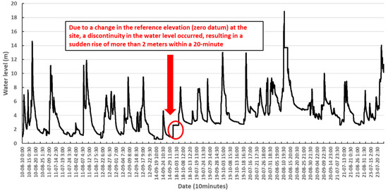
Figure 6.
A change in the gauge-zero reference at the monitoring site led to a water level discontinuity at the Gurye-gun (Songjeong-ri) site.
As a direction for future research, we aim to validate the proposed input data structuring method across a wider range of sites and address the uncertainty associated with forecasted rainfall and dam releases. Through this work, we seek to advance the developed algorithm for use in practical applications involving real-world flood forecasting operations.
Author Contributions
Funding acquisition, supervision, funding, data supply, revision editing, J.P.; original draft, G.L.; methodology, data curation, original draft, D.K.; conceptualization, methodology, data curation, original draft, writing, revising—review and editing, supervision, C.J. All authors have read and agreed to the published version of the manuscript.
Funding
It was prepared following the research work “GP2025-11” funded by the Korea Environment Institute (KEI).
Data Availability Statement
The data presented in this study are available upon request from the corresponding author. The data are not publicly available owing to our laboratory’s policy and confidentiality agreements.
Acknowledgments
This paper is based on the results of the research work “A Study on the Habitat Environment of Corbicula in the Lower Seomjin River through Empirical Investigation (2025-022)”, conducted by the Korea Environment Institute (KEI) upon the request of the Korea Ministry of Environment.
Conflicts of Interest
Darae Kim was employed by HECOREA. Gayeong Lee was employed by ECOLABS. The remaining authors declare that the research was conducted in the absence of any commercial or financial relationships that could be construed as a potential conflict of interest.
Appendix A
Table A1.
The results of parameter tuning performed during the LSTM training process via grid search-based CV algorithms with the original input data.
Table A1.
The results of parameter tuning performed during the LSTM training process via grid search-based CV algorithms with the original input data.
| Stations | Parameters | |||||
|---|---|---|---|---|---|---|
| Lead Time | Nodes | Learning-Rate | Batch_Size | Activation Function | Epochs | |
| Imsil-gun (Iljung-ri) | 3 h | 64 | 0.1 | 128 | Sigmoid | 30 |
| 6 h | 256 | 0.1 | 32 | Sigmoid | 10 | |
| 12 h | 128 | 0.1 | 64 | Sigmoid | 30 | |
| 24 h | 256 | 0.001 | 64 | Linear | 10 | |
| Gokseong-gun (Geumgok Bridge) | 3 h | 256 | 0.01 | 128 | Linear | 50 |
| 6 h | 64 | 0.1 | 64 | Sigmoid | 30 | |
| 12 h | 256 | 0.1 | 64 | Linear | 30 | |
| 24 h | 128 | 0.01 | 32 | Sigmoid | 50 | |
| Gokseong-gun (Yesung Bridge) | 3 h | 64 | 0.01 | 32 | Linear | 50 |
| 6 h | 16 | 0.001 | 32 | Sigmoid | 30 | |
| 12 h | 16 | 0.001 | 64 | Sigmoid | 30 | |
| 24 h | 256 | 0.001 | 128 | Sigmoid | 10 | |
| Gokseong-gun (Taean Bridge) | 3 h | 16 | 0.01 | 64 | Sigmoid | 50 |
| 6 h | 256 | 0.01 | 64 | Linear | 10 | |
| 12 h | 256 | 0.01 | 64 | Linear | 30 | |
| 24 h | 16 | 0.001 | 128 | Sigmoid | 30 | |
| Gurye-gun (Gurye Bridge) | 3 h | 16 | 0.01 | 128 | Sigmoid | 50 |
| 6 h | 16 | 0.1 | 64 | Sigmoid | 50 | |
| 12 h | 16 | 0.01 | 128 | Sigmoid | 50 | |
| 24 h | 256 | 0.01 | 32 | Linear | 10 | |
| Gurye-gun (Songjeong-ri) | 3 h | 256 | 0.01 | 32 | Linear | 30 |
| 6 h | 128 | 0.001 | 32 | Linear | 50 | |
| 12 h | 16 | 0.001 | 128 | Sigmoid | 30 | |
| 24 h | 128 | 0.1 | 32 | Linear | 50 | |
Appendix B
Table A2.
The results of parameter tuning performed during LSTM training via grid search-based CV algorithms using the enhanced input data with hybrid-modeled data.
Table A2.
The results of parameter tuning performed during LSTM training via grid search-based CV algorithms using the enhanced input data with hybrid-modeled data.
| Stations | Parameters | |||||
|---|---|---|---|---|---|---|
| Lead Time | Nodes | Learning-Rate | Batch_Size | Activation Function | Epochs | |
| Imsil-gun (Iljung-ri) | 3 h | 128 | 0.001 | 32 | Sigmoid | 50 |
| 6 h | 128 | 0.1 | 32 | Sigmoid | 50 | |
| 12 h | 64 | 0.001 | 32 | Sigmoid | 50 | |
| 24 h | 128 | 0.1 | 32 | Sigmoid | 50 | |
| Gokseong-gun (Geumgok Bridge) | 3 h | 32 | 0.1 | 32 | ReLU | 50 |
| 6 h | 256 | 0.1 | 64 | Sigmoid | 50 | |
| 12 h | 128 | 0.01 | 32 | Sigmoid | 50 | |
| 24 h | 64 | 0.1 | 32 | Sigmoid | 30 | |
| Gokseong-gun (Yesung Bridge) | 3 h | 32 | 0.1 | 32 | ReLU | 50 |
| 6 h | 32 | 0.1 | 32 | ReLU | 50 | |
| 12 h | 64 | 0.01 | 64 | Sigmoid | 30 | |
| 24 h | 16 | 0.01 | 32 | Sigmoid | 50 | |
| Gokseong-gun (Taean Bridge) | 3 h | 16 | 0.1 | 32 | ReLU | 50 |
| 6 h | 128 | 0.01 | 64 | Sigmoid | 50 | |
| 12 h | 256 | 0.1 | 32 | Sigmoid | 50 | |
| 24 h | 256 | 0.001 | 128 | Sigmoid | 50 | |
| Gurye-gun (Gurye Bridge) | 3 h | 64 | 0.01 | 32 | ReLU | 50 |
| 6 h | 64 | 0.1 | 32 | ReLU | 50 | |
| 12 h | 16 | 0.01 | 32 | ReLU | 50 | |
| 24 h | 16 | 0.1 | 64 | Sigmoid | 50 | |
| Gurye-gun (Songjeong-ri) | 3 h | 32 | 0.01 | 32 | ReLU | 30 |
| 6 h | 32 | 0.01 | 32 | ReLU | 30 | |
| 12 h | 64 | 0.001 | 32 | ReLU | 30 | |
| 24 h | 128 | 0.01 | 64 | ReLU | 50 | |
References
- Gao, Y.; Zhang, X.; Zhang, X.; Li, D.; Yang, M.; Hua, R.; Tian, J. Building check dams systems to achieve water resource efficiency: Modelling to maximize water and ecosystem conservation benefits. Hydrol. Res. 2020, 51, 1409–1436. [Google Scholar] [CrossRef]
- Government of Bihar; World Bank; Global Facility for Disaster Reduction & Recovery. Bihar Kosi Flood (2008) Needs Assessment Report; Government of Bihar: Patna, India, 2010. Available online: https://www.gfdrr.org/sites/default/files/publication/pda-2010-india.pdf (accessed on 16 September 2025).
- India Water Portal. Man-Made Floods in Orissa in September 2011—Key Issues Raised. 2011. Available online: https://www.indiawaterportal.org/agriculture/farm/man-made-floods-orissa-september-2011-key-issues-raised-water-initiatives-orissa (accessed on 16 September 2025).
- Schaper, D. 3 Reasons Houston Was A ‘Sitting Duck’ for Harvey Flooding. NPR. 31 August 2017. Available online: https://www.npr.org/2017/08/31/547575113/three-reasons-houston-was-a-sitting-duck-for-harvey-flooding/ (accessed on 29 September 2025).
- Lee, J.Y.; Son, H.J.; Kim, D.; Ryu, J.H.; Kim, T.W. Evaluating the hydrologic risk of n-year floods according to RCP scenarios. Water 2021, 13, 1805. [Google Scholar] [CrossRef]
- Lee, E.K.; Yi, S.Y.; Hong, J.H.; Lee, S.M.; Yoon, J.I.; Yi, J.E. Development of a reservoir operation model determining the pre-release strategy for flood events. J. Hydroinform. 2025, 27, 700–715. [Google Scholar] [CrossRef]
- Lee, D.Y.; Baek, K.O. Strategy for engancing flood capacity of Seomjin River Basin using both structural and non-structural measures. KSCE J. Civ. Environ. Eng. Res. 2024, 44, 683–694. (In Korean) [Google Scholar] [CrossRef]
- Ahn, J.M.; Lyu, S. Assessing future river environments in the Seomjin River Basin due to climate change. J. Environ. Eng. 2017, 143, 04017005. [Google Scholar] [CrossRef]
- Turkel, A.O.; Zaifoglu, H.; Yanmaz, A.M. Probabilistic modeling of dam failure scenarios: A case study of Kanlikoy Dam in Cyprus. Nat. Hazards 2024, 120, 10087–10117. [Google Scholar] [CrossRef]
- Zhou, Q.; Teng, S.; Situ, Z.; Liao, X.; Feng, J.; Chen, G.; Zhang, J.; Lu, Z. A deep-learning-technique-based data-driven model for accurate and rapid flood predictions in temporal and spatial dimensions. Hydrol. Earth Syst. Sci. 2023, 27, 1791–1808. [Google Scholar] [CrossRef]
- Li, X.; Xu, W.; Ren, M.; Jiang, Y.; Fu, G. Hybrid CNN-LSTM models for river flow prediction. Water Supply 2022, 22, 4902–4919. [Google Scholar] [CrossRef]
- Waqas, M.; Humphries, U.W. A critical review of RNN and LSTM variants in hydrological time series predictions. MethodsX 2024, 13, 102946. [Google Scholar] [CrossRef]
- Wei, X.; Wang, G.; Schmalz, B.; Hagan, D.F.T.; Duan, Z. Evaluation of transformer model and self-attention mechanism in the Yangtze River basin runoff prediction. J. Hydrol. Reg. Stud. 2023, 47, 101438. [Google Scholar] [CrossRef]
- Kratzert, F.; Klotz, D.; Brenner, C.; Schulz, K.; Herrnegger, M. Rainfall–Runoff Modelling Using Long Short-Term Memory (LSTM) Networks. Hydrol. Earth Syst. Sci. 2018, 22, 6005–6022. [Google Scholar] [CrossRef]
- Hu, C.; Wu, Q.; Li, H.; Jian, S.; Li, N.; Lou, Z. Deep Learning with a Long Short-Term Memory Networks Approach for Rainfall–Runoff Simulation. Water 2018, 10, 1543. [Google Scholar] [CrossRef]
- Rahimzad, M.; Nia, A.M.; Zolfonoon, H.; Soltani, J.; Mehr, A.D.; Kwon, H.H. Performance comparison of an LSTM-based deep learning model versus conventional machine learning algorithms for streamflow forecasting. Water Resour. Manag. 2021, 35, 4167–4187. [Google Scholar] [CrossRef]
- Le, X.H.; Ho, H.V.; Lee, G.; Jung, S. Application of long short-term memory (LSTM) neural network for flood forecasting. Water 2019, 11, 1387. [Google Scholar] [CrossRef]
- Mehedi, M.A.A.; Khosravi, M.; Yazdan, M.M.S.; Shabanian, H. Exploring temporal dynamics of river discharge using univariate long short-term memory (LSTM) recurrent neural network at east branch of Delaware River. Hydrology 2022, 9, 202. [Google Scholar] [CrossRef]
- Lee, S.W.; Kim, J.K. Predicting inflow rate of the Soyang River Dam using deep learning techniques. Water 2021, 13, 2447. [Google Scholar] [CrossRef]
- Hong, J.Y.; Lee, S.R.; Lee, G.J.; Yang, D.S.; Bae, J.H.; Kim, J.G.; Kim, K.S.; Lim, K.J. Comparison of machine learning algorithms for discharge prediction of multipurpose dam. Water 2021, 13, 3369. [Google Scholar] [CrossRef]
- Sharafkhani, F.; Corns, S.; Holmes, R. Multi-step ahead water level forecasting using deep neural networks. Water 2024, 16, 3153. [Google Scholar] [CrossRef]
- Sergio, R.L.C.; Fernando, S.; Ernest, B. Combining synthetic and observed data to enhance machine learning model performance for streamflow prediction. Water 2023, 15, 2020. [Google Scholar] [CrossRef]
- Sit, M.; Demiray, B.; Demir, I. Short-term hourly streamflow prediction with graph convolutional gru networks. arXiv 2021, arXiv:2107.07039. [Google Scholar] [CrossRef]
- Farfán-Durán, J.F.; Cea, L. Streamflow forecasting with deep learning models: A side-by-side comparison in Northwest Spain. Earth Sci. Inform. 2024, 17, 5289–5315. [Google Scholar] [CrossRef]
- Jung, S.H.; Cho, H.S.; Kim, J.Y.; Lee, G.H. Prediction of water level in a tidal river using a deep-learning based LSTM model. J. Korea Water Resour. Assoc. 2018, 51, 1207–1216. [Google Scholar] [CrossRef]
- Li, F.; Lv, M.; Li, H. Few-shot flood water level prediction based on mechanistic models and deep learning: A collaborative HEC-RAS-LSTM framework. E3S Web Conf. 2025, 628, 02006. [Google Scholar] [CrossRef]
- Andrei, M.R. Alterative hydraulic modeling method based on recurrent neural networks: From HEC-RAS to AI. Hydrology 2025, 12, 207. [Google Scholar] [CrossRef]
- Brunner, G. HEC-RAS, River Analysis System Hydraulic Reference Manual; U.S. Army Corps of Engineers: Davis, CA, USA, 2016.
- Hodson, T.O. Root-mean-square error (RMSE) or mean absolute error (MAE): When to use them or not. Geosci. Model Dev. 2022, 15, 5481–5487. [Google Scholar] [CrossRef]
- Moriasi, D.; Gitau, M.; Pai, N.; Daggupati, P. Hydrologic and water quality models: Performance measures and evaluation criteria. Trans. ASABE 2015, 58, 1763–1785. [Google Scholar] [CrossRef]
- Frame, J.M.; Kratzert, F.; Klotz, D.; Gauch, M.; Shalev, G.; Gilon, O.; Qualls, L.M.; Gupta, H.V.; Nearing, G.S. Deep learning rainfall-runoff predictions of extreme events. Hydrol. Earth Syst. Sci. 2022, 26, 3377–3392. [Google Scholar] [CrossRef]
- Tursun, A.; Xie, X.; Wang, Y.; Peng, D.; Liu, Y.; Zheng, B.; Wu, X.; Nie, C. Streamflow prediction in human-regulated catchments using multiscale deep learning modeling with anthropogenic similarities. Water Resour. Res. 2024, 60, e2023WR036853. [Google Scholar] [CrossRef]
- Hunt, K.M.R.; Matthews, G.R.; Pappenberger, F.; Prudhomme, C. Using a long short-term memory (LSTM) neural network to boost river streamflow forecasts over the western United States. Hydrol. Earth Syst. Sci. 2022, 26, 5449–5472. [Google Scholar] [CrossRef]
- Hou, S.; Wei, J.; Hou, M.; Xu, J.; Han, L. A hydrological knowledge-informed LSTM model for monthly streamflow reconstruction using distributed data: Application to typical rivers across the Tibetan plateau. J. Hydrol. 2025, 649, 132409. [Google Scholar] [CrossRef]
- Nevo, S.; Morin, E.; Rosenthal, A.G.; Metzger, A.; Barshai, C.; Weitzner, D.; Voloshin, D.; Kratzert, F.; Elidan, G.; Dror, G.; et al. Flood forecasting with machine learning models in an operational framework. Hydrol. Earth Syst. Sci. 2022, 26, 4013–4032. [Google Scholar] [CrossRef]
Disclaimer/Publisher’s Note: The statements, opinions and data contained in all publications are solely those of the individual author(s) and contributor(s) and not of MDPI and/or the editor(s). MDPI and/or the editor(s) disclaim responsibility for any injury to people or property resulting from any ideas, methods, instructions or products referred to in the content. |
© 2025 by the authors. Licensee MDPI, Basel, Switzerland. This article is an open access article distributed under the terms and conditions of the Creative Commons Attribution (CC BY) license (https://creativecommons.org/licenses/by/4.0/).