Links Between Extremes in GRACE TWS and Climate Patterns Across Iberia

Abstract

The Iberian region relies heavily on groundwater and is highly vulnerable to climate variability, making it crucial to understand factors influencing water availability. The aim of this research was to assess how large-scale climate patterns affect total water storage anomalies (TWSAs) in Iberia, particularly in relation to persistent droughts and floods. To address this, I analyzed TWSAs derived from a reconstructed dataset (GRACE-REC) spanning from 1980 to 2019, first at the scale of the entire Iberian Peninsula and then across its main river basins. The links between the North Atlantic Oscillation (NAO), East Atlantic (EA) and Scandinavian (SCAND) patterns, TWSAs, and hydrological extremes were quantified using wavelet and principal component analysis. The results reveal that the NAO exerts the strongest multiyear influence on TWSAs, with periodicities of approximately 10 and 6.5 years, particularly in the southern river basins (Tagus, Guadiana, and Guadalquivir). EA and SCAND have stronger influences in the northern basins (Douro, Minho, and Ebro), driving 2- to 3.5-year cycles. Coupled phases of climate patterns, such as NAO+ and EA− (or SCAND−), correspond to extreme droughts, whereas NAO− and EA+ (or SCAND+) correspond to wet conditions.

1. Introduction

The assessment of hydrologic extremes is increasingly important due to the rising frequency of extreme events and the likelihood of their wider occurrence in the future [1,2,3]. The Iberian Peninsula is prone to droughts due to its Mediterranean climate, which are marked by extended dry periods and scarce water resources [4,5]. Long-term hydrological droughts in the region are well documented as having extensive impacts on agriculture, hydropower generation, domestic water supply, and ecosystems [6,7,8,9]. Projections of decreasing trends in water availability during the 21st century, due to reduced precipitation and increased potential evapotranspiration, are particularly acute in Iberia which has been identified as a Mediterranean climate change hotspot [3] and where climate projections for 2041–2070 forecast increasing frequency and severity droughts under all emissions scenarios [4,10,11]. These conditions will naturally exacerbate water shortages and groundwater abstraction, potentially leading to aquifer depletion [12,13]. On the other hand, floods in the Iberian Peninsula are a recurring natural hazard, often driven by persistent large-scale precipitation events, as noted in the literature [6,14]. The occurrence of intense and prolonged precipitation in this region is dominated by large-scale atmospheric circulation patterns and large traveling low-pressure systems during winter months. The passage of atmospheric rivers (ARs), that is, long, narrow corridors of concentrated moisture transport and the occurrence of cut-off lows are often associated with torrential rains and subsequent flooding, especially in coastal and mountainous area [15,16,17].

The Gravity Recovery and Climate Experiment (GRACE) satellite mission provides measurements of the Earth’s gravity field reflecting mass changes in the Earth [18]. Over land, these changes in mass are mainly due to changes in total terrestrial water storage (TWS), an integrated measure of water storage that includes snow, surface water, soil moisture, and groundwater [19,20,21]. GRACE is particularly valuable for detecting trends in groundwater storage from space, allowing us to overcome the lack of on-site groundwater measurements while providing the advantage of basin-integrated estimates. Over the last two decades, GRACE-derived data have been shown to match in situ measurements of groundwater levels [22,23,24] and been used to quantify the trends and interannual variability of groundwater at some of the largest aquifers in the world [25,26,27,28,29]. The direct use of GRACE data for near-real-time applications at small spatial scales (e.g., water basin) has been questioned due to their large latency (45 days), monthly aggregation, and coarse spatial resolution (one degree) [30], but some of these limitations can be overcome by data assimilation into land-surface models [29]. Furthermore, the TWS anomaly (TWSA), defined as the difference between the current TWS and the historical mean (baseline) for a given time period, has emerged as a comprehensive indicator of hydrological extremes [31,32,33,34,35]. TWSA is recognized as a valuable indicator of the slow-responding components of the water cycle and is currently being used as a proxy of groundwater drought in the Copernicus Global Drought Observatory [36] and in drought monitoring applications such as the groundwater and soil moisture conditions maps in the United States [18]. In Iberia, TWSA is strongly correlated with meteorological indices such as the standardized precipitation index for an accumulation period of 12 months (SPI-12), making it a reliable indicator for assessing large-scale and persistent hydrological droughts [37].

Many studies have evaluated the importance of climate patterns such as the El Niño—Southern Oscillation (ENSO) in driving the large-scale spatial distribution and temporal variability in precipitation and temperature, and hence the variations of TWS over seasonal to decadal timescales [38,39,40,41,42,43,44,45,46]. However, analyzing climate patterns requires long-term data (at least 30 years) to capture decadal variability, and GRACE satellite data have only been available since 2002. While global hydrological models (e.g., land-surface models) offer multi-decadal simulations, their exclusion of groundwater cycles and limitations in data-sparse regions lead to significant uncertainties, making them inappropriate for representing natural interannual TWS variability [27]. Therefore, this study utilized GRACE-REC, a statistical model output proven to accurately capture climate-driven TWS interannual variations [47]. GRACE-REC uses meteorological data (precipitation, temperature) as input, is trained with GRACE observations, and is calibrated by removing the linear trend and seasonal signal to isolate natural interannual variability. Although GRACE-REC data span from 1901 to mid-2019, I focused on the 1980–2019 period to align with previous studies analyzing correlations between climate patterns and in situ groundwater records in Portugal [48,49].

In the Iberian Peninsula, the North Atlantic Oscillation (NAO) and East Atlantic (EA) and Scandinavian (SCAND) patterns are the three main modes of variability driving winter precipitation, river flow, and therefore surface and subsurface water storage [50,51,52]. These patterns or modes of variability are characterized by indices that measure the strength of atmospheric pressure anomalies. Positive and negative phases of the indices, defined by values above or below given thresholds (e.g., NAO+ is defined for aggregates of winter month indices above 0.5), are generally associated with either wet or dry conditions. Previous studies have shown that wintertime NAO+ and EA− phases potentiate droughts in Iberia, the opposite occurring for NAO− and EA+ phases [53]. However, few studies have recognized the importance of interactions amongst climate patterns, and only recently did we become aware that conjunctions between climate patterns phases may indeed prompt anomalous precipitation and hydrological extremes [54,55,56], offering an opportunity for potential recurrent drought prediction [57,58].

A prior evaluation of GRACE data for water resource management in Iberia demonstrated GRACE’s ability to consistently represent the Iberian hydrological cycle, making it a valuable tool for monitoring climate-related water mass transport at the peninsula scale [59]. It was concluded that GRACE is effectively capable of capturing the regionally integrated groundwater storage changes with good accuracy, and also able to capture the multi-year deficits and surplus resulting from the natural climate fluctuations. The authors suggested that the observed multi-year deficits and low-frequency cycles are related to low-frequency oscillations in the amount of precipitation, driven by large-scale climate patterns such as the NAO and EA, but did not attempt to demonstrate this relationship. This work completes the previous study and presents the first analysis of TWSA derived from GRACE in Iberia aiming to demonstrate and quantify their dependence on large-scale climate patterns such as the North Atlantic Oscillation (NAO), East Atlantic pattern (EA), and Scandinavian pattern (SCAND). By exploring these connections, this work assesses the potential of GRACE satellite data in evaluating total available water resources, particularly under climate extremes. A novelty lies in the use of GRACE-reconstructed data extending back to 1980, allowing for a long-term perspective on TWS variability. The nonstationary relationships between climate indices and TWS anomaly are investigated using wavelet transform methods and principal component analysis. By integrating GRACE data with teleconnection indices, we can better understand recurrent droughts and floods and improve water resource management strategies to address natural and anthropogenic pressures.

2. Materials and Methods

2.1. GRACE and Climate Data

This study analyzed the spatial average of GRACE data over the entire Iberian Peninsula, as well as over five individual subdomains defined by the largest Iberian river basins, aggregated to match the Köppen–Geiger climate divisions (Figure 1). There is a natural divide between the “wet Iberia” in the north and the “dry Iberia” in the south, the former including the Douro, Minho, and Ebro rivers, with considerably higher discharges than the latter, including the Tagus, Guadiana, and Júcar rivers [4,50]. GRACE data products are processed and provided by various research centers such as the Center for Space Research (CSR), the Jet Propulsion Laboratory (JPL) and the Goddard Space Flight Center (GSFC). A snapshot of the CSR-GRACE Mascon product, which has been shown in previous studies to be the product that best aligns with the hydrological balance of the Iberian Peninsula [58], is shown in Figure 1c. However, the GRACE mission, which began in 2002, has a limited temporal coverage. Since climate variability studies typically require at least 30 years of data, GRACE alone is insufficient for such analyses. To overcome this limitation, I used GRACE-REC, a data reconstruction product published in 2019 [47]. GRACE-REC employs a statistical model trained on GRACE observations to reconstruct historical climate-driven changes in TWS using past and near-real-time meteorological datasets. Previous studies have shown that GRACE-REC effectively captures interannual climate-driven TWS variations, particularly at the catchment scale [27,28,40].

The GRACE-REC dataset is available at a spatial resolution of 0.5° and includes daily and monthly records from 1901 to the present. It is derived from two GRACE products (GSFC and JPL) and three different meteorological forcing datasets, resulting in six reconstructed TWS datasets with 100 ensemble members each. For this study, I used the reconstructed GSFC solution driven by ERA5 precipitation data, as it has shown slightly better performance than JPL-based reconstructions using other meteorological datasets. The GRACE-REC reconstruction does not include trends or seasonal signals. TWSA has been extracted for Iberia, and water storage changes at monthly scale are measured in millimeters of water layer thickness (lwe) (Figure 1d). To estimate groundwater storage, soil moisture would need to be subtracted from TWSA. However, due to significant uncertainties in soil moisture data, this estimate is left for future research.

To analyze large-scale atmospheric variability, I used standard low-frequency climate indices obtained from NOAA’s Climate Prediction Center [64] for the period 1980–2019. The indices are derived from the 500 hPa geopotential height field across the Northern Hemisphere using rotated principal component analysis at a monthly scale (Figure 2a). The NAO is characterized by a meridional pressure dipole between Iceland and the Azores, exhibiting interannual and decadal variability [51]. In its positive phase (NAO+), high pressure dominates over the Azores and low pressure over Iceland, leading to colder, drier winters in southern Europe and warmer, wetter winters in northern Europe. The negative phase (NAO−) reverses these effects. However, the NAO’s impact on surface climate is nonstationary and depends on interactions with other teleconnections such as EA and SCAND [48]. The EA pattern also has a dipole structure, but it is shifted southeastward relative to the NAO. In its positive phase (EA+), it is associated with low pressure over the North Atlantic, leading to higher-than-average precipitation in Northern Europe [53]. Figure 2b displays the winter aggregates (DJFM) of the NAO, EA, and SCAND indices, computed as the average values from December to March. The positive and negative phases are classified based on index values above the third tercile and below the first tercile, respectively [64].

The standardized precipitation evapotranspiration index (SPEI), which is based on precipitation and temperature data, has the advantage of including the effect of temperature variability on drought assessment and is particularly useful to quantify drought in the Iberian Peninsula [65]. The SPEI can be computed for different accumulation periods to monitor meteorological (<6 months), agricultural (e.g., 6–12 months), and hydrological droughts (e.g., 12–24 months). For comparative purposes with GRACE data, this study used the SPEI-6 and SPEI-12 time series spatially averaged over Iberia and downloaded from the Global SPEI database [66].

2.2. Methods of Analysis

The GRACE-REC dataset provides reconstructed, detrended, and de-seasonalized terrestrial water storage anomaly (TWSA) data in NetCDF grid format. After extracting the data for the Iberian Peninsula, a spatial averaging process was applied to generate monthly time series spanning from 1980 to 2019. This resulted in one time series representing the spatial average across the entire Iberian domain and five additional time series corresponding to the averages for each of the selected river basins: Douro and Minho, Tagus and Guadiana, Ebro, Jucar, and Guadalquivir. To recognize extreme hydrological events from TWSAs, this study calculated the GRACE drought index as the standardized departure from GRACE climatology over the study period (1980–2019):

$${GGDI}_{i,j}={\displaystyle \frac{{TWSA}_{i,j}-\overline{{TWSA}_j}}{{\sigma }_j}}$$

(1)

with i ranging from 1980 to 2019, where $\overline{{TWSA}_j}$ and ${\sigma }_j$ are the mean and standard deviation of TWSAs for month j. This approach has been employed in previous studies to quantify drought-induced total water storage deficits using GRACE data [33,67]. However, it is equally effective for identifying water storage excess, serving as a wetness index [32].

The GRACE and climate indices time series were investigated using several analytical techniques to characterize their temporal structure (periodic components of their signal), namely continuous wavelet transform (CWT) and wavelet coherence (Figure 3).

The CWT is a powerful method of time-series analysis especially suited to analyzing nonstationary signals that have temporal variations in both amplitude and frequency [68]. The method is usually applied in hydrology to assess how the dominant modes of variability change over time, to reduce noise in chaotic time series, and to detect localized or intermittent events. This study used the MATLAB R2024b implementation based in the Morlet wavelet. The local wavelet power spectrum, defined as the absolute value squared of the wavelet transform, displays the distribution of the variance of the time series as a function of time. The cone of influence (black parabolic lines) defines the region where the edge effects render the results less reliable. Statistical significance was estimated using the Monte Carlo method. The global wavelet spectrum is an average in time of the wavelet spectrum and shows the net changes in variance over the entire recording period.

The wavelet coherence definition is similar to a localized correlation coefficient between two continuous wavelet transforms in time–frequency space [69]. This method has been applied to identify time-localized common oscillatory behaviors between the climate indices (NAO, EA, and SCAND) and GGDI at both the whole Iberia and river basin scales, as is shown in wavelet transform coherence (WTC) plots. The wavelet coherence was computed at the 95% confidence level using the algorithm described in Grinsted et al. [70]. The direction of the arrows in the wavelet cross-spectrum represents the relative time lag between synchronized components. When two time series exhibit a positive correlation and are in phase, the arrows point to the right, whereas they point to the left when the correlation is negative, and the series are in antiphase. Areas in time–frequency space with large common power and regular phase relationships are likely to have a cause–effect relationship between the time series.

3. Results

3.1. Indices of Hydrological Extremes and Temporal Patterns of TWS Changes

The TWS anomaly averaged over Iberia from 1980 to 2019 exhibits both annual and multi-annual variations, ranging between −40 and 40 mm of water layer thickness (Figure 4a). The GRACE reconstructed product and the CRS GRACE solution, the latter only available from 2003 onwards, show reasonable agreement, reinforcing confidence in the use of the reconstructed dataset.

The GGDI (Figure 4b), which quantifies deviations in total water storage from climatology, fluctuates around the zero line, indicating periods of both water surplus (positive values) and water deficit (negative values). Purple and orange horizontal lines mark the thresholds of −1.28 and 1.28, often used in the literature as thresholds for severe events that correspond to approximately 10% of the extreme dry and wet cases [6,67]. The same threshold lines appear in Figure 4c, which shows the SPEI-12 and SPEI-6 indices for a qualitative comparison with GGDI. The SPEI is also clustered around zero, with negative values indicating drier-than-normal conditions and positive values indicating wetter-than-normal conditions. Both GGDI and SPEI show a general agreement in identifying periods of drought and wetter conditions. This agreement is more clearly illustrated in Figure 4d, which shows the three indices superimposed. When GRACE indicates water deficit (negative GGDI), SPEI indices also tend to show negative values, suggesting dry conditions. Conversely, positive GGDI values often align with positive SPEI values, indicating wetter periods. The shaded bands around the severe event thresholds, representing a tolerance that includes events classified from moderate to exceptional, are reached in both GRACE and SPEI plots at similar times. This suggests that both GRACE-derived GGDI and SPEI indices are capturing drought and wet events with reasonable consistency.

However, there are differences in the magnitude and timing of the peaks and troughs between the GGDI and SPEI plots. SPEI-6 shows more rapid fluctuations compared to SPEI-12, as it reflects shorter-term variations, while SPEI-12 integrates over a longer period. The GRACE-based index, on the other hand, reflects changes in total water storage, which often have a different temporal response and a different level of intensity or magnitude. Meteorological droughts, for instance, indicated by precipitation deficits and reflected more quickly in SPEI-6, may not immediately translate to hydrological droughts (reflected in TWSA and GGDI), especially if groundwater reserves buffer short-term precipitation deficits. A quantitative comparison between SPEI and GGDI is out of the scope of the present study, but their differences are further addressed in Section 4.

The statistical properties of total water storage anomalies are more clearly interpreted using the CWT analysis, which allows analysis of both time and frequency information simultaneously (Figure 5). The CWT spectrum (Figure 5b) shows the temporal distribution of the power (variance) of the GGDI time series in Iberia as a function of period (scale) over the 30 years of analysis in a color scale that goes from blue (minimum) to yellow (maximum). The power (variance) of the continuous wavelet transform of GGDI is dimensionless because GGDI is a normalized index. The picture displays the evolution in time of the dominant modes of variability and the occurrence of large anomalies in total water storage corresponding to the most intense blue and yellow patches. The three main modes of variability with enough persistence and amplitude to be statistically significant (within white contours) have power concentrations with periods in the 10- to 13-year band (between 1983 and 2007), at 6.5 years (between 1993 and 2006), and at 3.5 years (between 2000 and 2015). At smaller scales with less energy, one can observe several scattered peaks at periods of less than 1 year, as, for instance, in 2001, which was an anomalously wet year. The global spectrum is obtained by integrating the CWT spectrum over the period of study (1980–2019), allowing us to easily identify the frequencies that contribute most significantly to the overall signal. When averaged over time, only two variability modes remain statistically significant at the 5% level, peaking at 3.5 and 10 years (Figure 5a).

3.2. Links Between Hydrological Extremes and Climate Indices

Figure 6 shows the wavelet coherence between the NAO, EA, and SCAND climate indices and the GGDI. Each climate index exhibits consistent phase relationships at characteristic periods, although sometimes restricted to specific time windows: NAO at long-term periods of 10–13 years, EA at a 3.5-year periodicity, particularly after 2005, and SCAND at periods of 2–6 years, mainly before 2005. Among these, NAO and SCAND exert the most widespread influence over Iberia, showing statistically significant coherence patches at multiple multiannual periodicities. Regarding the phase angle, there is a dominant horizontal anti-phase (180°) relationship between NAO and GDDI, which aligns with expectations. It is well known that during NAO-negative phases low-pressure systems in the North Atlantic are shifted southwards, leading to increased precipitation and increased river discharges in Iberia [50]. Thus, the out-of-phase relationship is in agreement with the fact that precipitation, aquifer recharge, and hence total water storage on land are negatively correlated with NAO. In contrast, EA and SCAND show arrow patterns that are mostly diagonal or pointing downward, indicating that changes in these indices either precede or follow shifts in the TWS time series.

Previous studies have shown that NAO, EA, and SCAND couplings, which occur when two or more of these indices are in opposite phases, impact extremes in groundwater storage [48]. Specifically, NAO+ EA− and NAO+ SCAND− are directly linked to major droughts, while NAO− EA+ and NAO− SCAND+ are associated with wetter-than-normal conditions. Similar links with TWS changes can be visually analyzed by comparing the timeline of GGDI events exceeding threshold limits, along with the timing of the coupled phases of climate patterns (Figure 7). Extremes in SPEI-6 and SPEI-12 (indices > 1.28 for wet events in Figure 7a and <−1.28 for dry events n Figure 7b) are also shown for comparison. Synchronicity occur when coupled phases, marked by bars in the bottom plots, align with extremes marked by lines and dots in the SPEI-6, SPEI-12, and GGDI plots.

The larger extreme events are those with greater intensity (more extreme index values) and longer duration (more consecutive months exceeding the threshold). Some of the larger extreme events coincide across multiple indices, for instance, the wet extreme in 2001 (Figure 7a) and the dry extreme in 1995 (Figure 7b). Extremes identified by GGDI do not always coincide with extremes in either SPEI-6 or SPEI-12, and when they do, they often show varying degrees of lag. This is not surprising, as meteorological extremes captured by SPEI may take time to manifest as hydrological extremes in GGDI. As precipitation moves through the different compartments of the hydrological cycle (for instance, soil moisture, streams, rivers, and groundwater) changes may be smoothed out during the process of propagation. The comparison between GGDI and SPEIs will be explored further in the next section.

Focusing on the links between GGDI and climate patterns, there is a clear coincidence in six out of the eight wet-phase couplings occurring during the study period, namely in 1985, 1996, 1998, 2001, 2010, and 2013 (Figure 7a). Considering a possible delay of nearly one year between GGDI and the wet phases in 1987 and 2003, this would result in a 100% match. As shown in Figure 7b, GGDI extremes align with five out of the seven years of dry-phases (1983, 1993, 1995, 2000, and 2012), indicating a slightly weaker performance of GGDI in detecting droughts compared to wet extremes. A possible explanation may be that wet events, which typically have high intensity and short duration, are more readily identifiable in TWS changes than dry events, which tend to have a slower onset and require longer duration deficits. It is evident that not all the extreme events detected by the indices, most notably the 2005 drought, are linked to coupled climate patterns. Furthermore, synchronicity does not necessarily mean causality, as discussed in the next section.

The impact of coupled phases is better illustrated in Figure 8, which displays the GRACE TWS anomalies averaged over years of positive and negative phases. For example, TWS variations for NAO− EA+ correspond to monthly values averaged over years with simultaneous NAO+ and EA− phases. Figure 8 clearly shows that maximum (wet) water storage anomalies occur in years when NAO− coincides with either SCAND+ or EA+ phases (notably, many SCAND+ and EA+ years overlap), while minimum levels (dry) occur during NAO+ and either EA− or SCAND− combinations. The difference in TWS between dry phases (NAO+ EA−/SCAND−) and wet phases (NAO− EA+/SCAND+) is maintained throughout the year, but it is most evident between January and May, since precipitation in Iberia falls essentially during the extended winter season and summer has always negative anomalies.

3.3. Spatial Variability in TWS–Climate Links

When considering the spatially averaged TWS anomalies within each river basin the results obtained are essentially the same, that is, the anomalies are consistently below the mean (black line) in years of coupled NAO+ EA−/SCAND− and above the average in years of NAO− EA+/SCAND+ combinations (Figure 9). However, the range in the TWS difference between wet and dry years is more notorious in the Douro (10 mm), Tagus (20 mm) and Guadalquivir (5 mm) than in the Ebro (<5 mm), and Júcar (<2 mm) river basins.

The influence of patterns in the Ebro and Júcar basins is very small, with just a few and scattered patches showing correlations between the GRACE GGDI and the NAO, EA, and SCAND indices (Figure 10). The weak correlation may be due to the smallness of these basins, which prevents GRACE from capturing the dynamics of TWS. However, it may also be attributed to more complex precipitation patterns caused by topography or atmospheric rivers.

Spatial variations are more interesting to analyze in the other basins (Figure 11), as they exhibit consistent patterns like those observed on average for the Iberian Peninsula (Figure 6). The coherence patches in the Tagus and Guadalquivir river basins are clearly very similar, indicating more homogeneous climate pattern influences. This can be easily explained by the fact that these southern Iberia regions share the same climatic classifications (Figure 1). In contrast, the Douro basin shows slightly different links with the indices, with a greater influence from SCAND and a weaker and less frequent influence from NAO with a variability period of approximately 6.5 years. Interestingly, EA is associated with longer-term variability (with periods of around 10 years) in the northern Iberian Peninsula, affecting both the Douro and Ebro basins.

4. Discussion

4.1. Comparisons Between SPEI-6, SPEI-12 and GGDI

Wet and dry hydrological extremes in the Iberian Peninsula have been studied at many different spatial and temporal scales and using a great variety of methodological approaches (e.g., [7,13,14,15,16,17,71,72]). A recent study ranked the top 10 most widespread dry and wet events in Iberia between 1901 and 2016 using SPEI at different accumulation time scales (6, 12, 18, and 24 months) [6]. The most extreme wet events listed in that study (2001, 2010, 2013) align well with the events in Figure 7a. However, many of the droughts listed in [6] do not match the SPEI-6 or SPEI-12 events identified in Figure 7b (e.g., 1990, 1993, 2000, 2003). This discrepancy likely arises from differences in data sources and methodologies. In [6], SPEIs were computed from gridded data from the Climatic Research Unit (CRU), and extreme events were ranked based on both affected areas, defined by SPEI values exceeding a specific threshold, and intensity at each grid point. In contrast, the SPEI-6 and SPEI-12 time series used in the present study were taken from the SPEI global database and have been spatially averaged over the Iberian Peninsula, missing the spatial heterogeneity.

The timescale is crucial and explains why extremes in SPEI-6 do not always coincide with those in SPEI-12, or GGDI (Figure 7). SPEI-6 is more sensitive to short-term fluctuations and consequently more able to capture higher-frequency and intense extreme events. SPEI-12, in contrast, is associated with prolonged conditions, making it less responsive to short-lived events. Comparing GGDI with SPEI-6 and SPEI-12 shows that in some cases, GGDI aligns more closely with one than the other (Figure 4 and Figure 7). GRACE-based indices measure the sum of various water storage components, including surface water, soil moisture, and groundwater, each of which responds to precipitation and evapotranspiration changes at different rates [29]. Soil moisture reacts relatively quickly to rainfall, aligning with shorter timescale indices like SPEI-6, whereas groundwater responds more gradually, aligning better with longer indices like SPI-12. Other studies demonstrate that the correlation between GRACE data and precipitation-based indices varies across space and time, as the response of total water storage to precipitation anomalies depends on regional characteristics and timescales [31,67]. Local factors such as catchment properties and geological conditions influence how rivers, aquifers, and other storage components react to rainfall [24,25,46,73,74]. Thus, the optimal SPEI timescale for best correlations with GRACE-based indices depends on the dominant water storage dynamics in each region. For instance, while SPI-12 is generally optimal for GRACE TWS correlation over Europe, spatial variability means that different accumulation periods are more suitable in specific areas [37].

Hydrological extremes develop over time as precipitation anomalies propagate through the hydrological cycle [75]. When considering drought, these processes include pooling, where multiple short meteorological events combine into a longer hydrological drought; attenuation, where severity decreases as anomalies move through storage components; and lag effects, where soil moisture and groundwater respond later than meteorological droughts [76]. This can explain the weaker performance of GGDI in detecting droughts compared to wet extremes in the present study. A weaker performance of GRACE to detect droughts when compared to wet conditions has also been found in previous research [31]. Each drought index is based on different aspects of the hydrological cycle and uses its own scale and set of thresholds to define severity.

One of the advantages of using GRACE-based indices is that unlike methods focusing solely on surface water or meteorological data, they offer a more comprehensive assessment of water availability because they include the response of subsurface reservoirs [29,77]. However, different groundwater systems, even within small regions, exhibit varying lag times and attenuation in response to meteorological extremes [74]. Anthropogenic groundwater use can further complicate the relationship between GGDI and meteorological indices [12,78].

4.2. Links Between TWS, GGDI, and Climate Patterns

Wavelet analysis revealed that NAO exerts a strong multi-year influence on TWS changes, with an oscillatory period of approximately 10 years. This aligns with previous studies that have identified similar cycles in precipitation, streamflow, and groundwater levels across Iberia, with periodicities ranging from 8 to 11 years [5,49,51], demonstrating that NAO is a key driver of hydrological variability, affecting both surface and subsurface water reservoirs. Additionally, EA and SCAND show significant coherence with GRACE anomalies, though their influence varies spatially and temporally. EA exhibited a 3.5-year periodicity, particularly pronounced after 2005, while SCAND was more dominant before 2005. Previous studies showed that NAO explains 19% of the total precipitation variation in Iberia, whereas EA and SCAND jointly explain 46% of the annual precipitation variability in the region [5].

The results of the present study also highlighted that coupled climate pattern phases, such as NAO+ EA− (or NAO+ SCAND−) and NAO− EA+ (or NAO− SCAND+), potentially contribute to extreme drought and wet conditions captured by GGDI. A visual analysis of coinciding events was used in this study. Other methods such as breakpoint detection and synchronization analysis [31] offer a more objective and adaptive approach to identifying abrupt hydrologic changes and can be used in future studies. However, while synchronization analysis may reveal significant temporal links, it does not imply causation, as hydrologic responses involve complex processes that cannot be inferred solely from statistical concurrence. The 2005 drought, for instance, is the most notable example of a drought that is not simply related to phases of climate patterns. The 2004–2005 drought in the Iberian Peninsula has been classified as exceptional and explained by a strengthening stage of NAO toward its positive phase in combination with an abnormal atmospheric blocking situation during spring [79].

Spatial analysis of climate–GGDI relationships in the present study revealed considerable heterogeneity across Iberian river basins. Weaker coherences found in the Ebro and Júcar river basins are likely due to their smaller dimensions, the influence of topography, and complex hydrological processes. This is consistent with previous findings indicating that climate teleconnections exert stronger control over GRACE hydrology in large lowland basins, where precipitation and evapotranspiration drive long-term water balance trends [26]. Additionally, atmospheric rivers (ARs) significantly contribute to extreme precipitation in these regions, complicating the relationship between large-scale climate patterns and water storage variability [15].

Previous GRACE studies have successfully linked TWS variability to large-scale climate patterns all over the world, for instance, in Africa [40], Asia [42], South America [45] and North America [46], demonstrating that ENSO, NAO, and other teleconnections exert significant control over regional water storage trends. Our findings extend this understanding to Iberia, confirming that GRACE-derived TWS effectively captures interannual and decadal climate-driven hydrological variability. However, challenges remain in using GRACE for basin-scale hydrological analysis due to signal leakage and data processing uncertainties, as noted in previous studies (e.g., [40,45]). The coarse spatial resolution of GRACE data limits their ability to resolve small-scale processes, calling for the use of downscaling techniques and complementary datasets, such as hydrological data from land-surface models or InSAR data (e.g., [80,81]). Despite these limitations, our study confirms that GRACE provides valuable insights into climate-driven water storage dynamics at regional scales. Given the projected intensification of extreme hydrological events under future climate change scenarios, integrating GRACE TWS anomalies with climate pattern forecasts could enhance early warning systems and adaptive water management strategies [32,40]. Future research should focus on refining regional-scale TWS estimates by integrating GRACE with high-resolution hydrological models and other remote sensing datasets. Additionally, further investigation into the role of coupled climate models and their nonstationary influences on Iberian hydrology is needed, particularly considering potential regime shifts in climate variability [48].

5. Conclusions

This study provides the first analysis of total water storage anomalies (TWSAs) derived from GRACE in Iberia aiming to demonstrate and quantify their dependence on large-scale climate patterns such as the North Atlantic Oscillation (NAO), East Atlantic pattern (EA), and Scandinavian pattern (SCAND). The main conclusions are as follows:

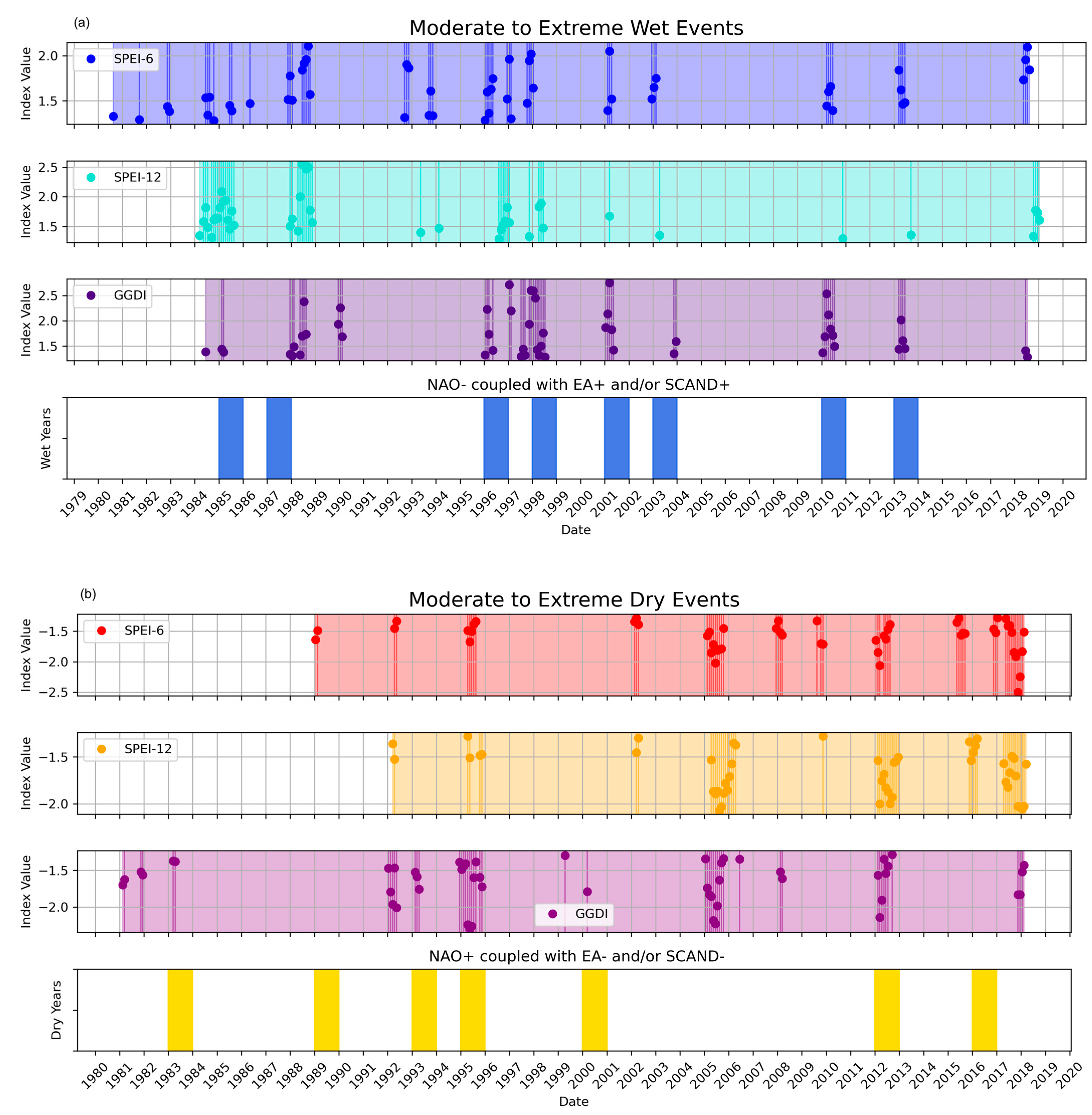
• The GRACE drought index (GGDI), which is derived from TWSA, shows good overall agreement with other drought indices like SPEI-12 and SPEI-6 in identifying periods of drought and wetter conditions. While there are differences in the magnitude and timing of extreme events due to SPEI reflecting meteorological conditions and GGDI representing total water storage (including surface water, soil moisture, and groundwater), GGDI effectively serves as a comprehensive indicator of hydrological extremes in the Iberian Peninsula.
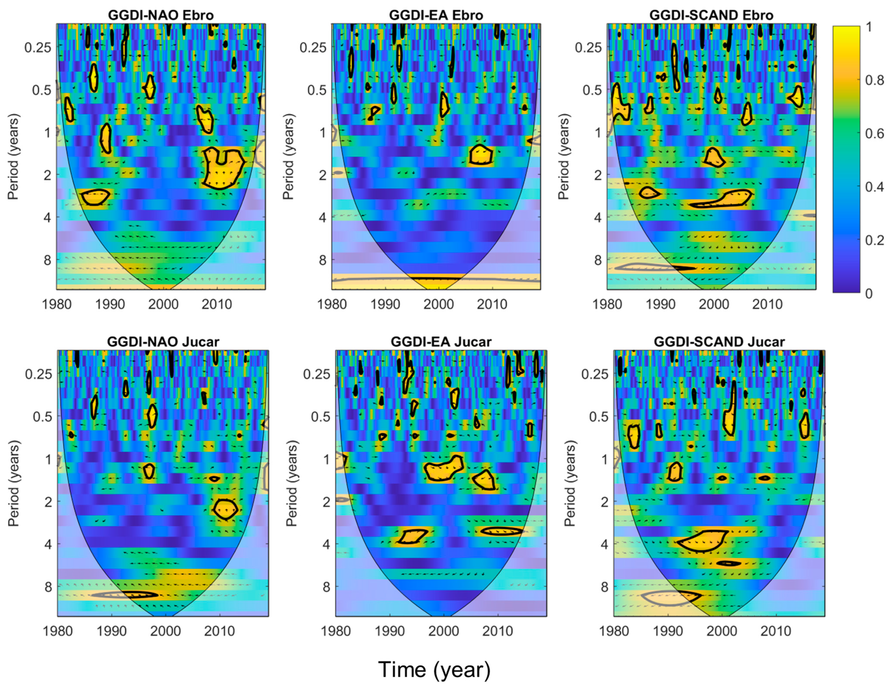
• The study also confirms that NAO, EA, and SCAND exert a strong influence on TWSA and GGDI across the Iberian Peninsula. Wavelet analysis reveals that NAO controls GGDI fluctuations with a dominant oscillatory period of approximately 10 years and that EA and SCAND patterns control fluctuations with shorter periodicities (2–3.5 years).
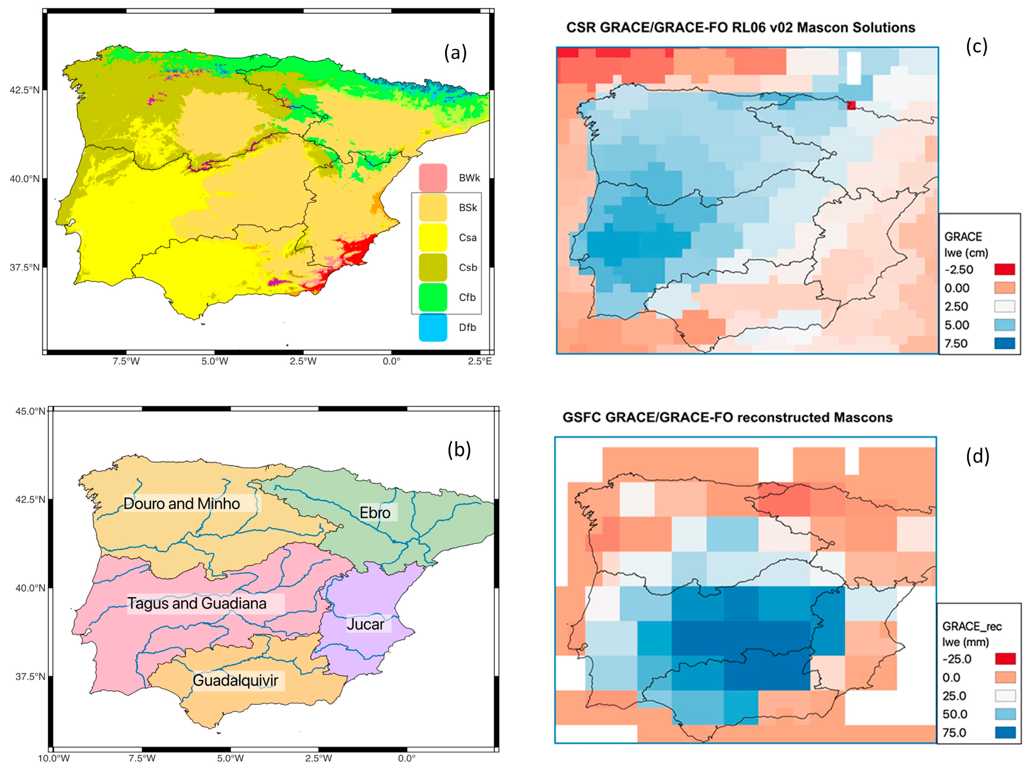
• The influence of climate patterns on TWSA varies spatially across the Iberian Peninsula. In the southern river basins (Tagus and Guadalquivir), responses are more homogeneous, showing a greater influence of NAO. The Douro basin shows a greater influence from the SCAND pattern and a weaker NAO influence. The smaller basins (Ebro and Júcar) display weaker correlations with NAO, EA, and SCAND, likely reflecting their smaller dimensions and the presence of more complex, localized precipitation patterns influenced by other factors like topography and atmospheric rivers.
• The analysis of GGDI further demonstrates a strong alignment between GRACE-derived hydrological extremes and coupled phases of the climate patterns. Specific coupled phases such as NAO+ EA− or NAO+ SCAND− are linked to droughts, while NAO− EA+ or NAO− SCAND+ are linked to wet conditions. This suggests that GRACE-derived indices can reflect the impact of these climate pattern interactions on hydrological extremes over time.
• These relationships indicate that monitoring climate phase interactions using GRACE data can potentially improve long-term drought and flood predictions, offering valuable insights for water resource management and early warning systems. However, it is important to note that while GRACE data can capture the synchronization between climate patterns and hydrological responses, synchronization does not imply causation, and further research is needed to isolate the direct impact of climate patterns from other possible influencing factors.

References

1. Sillmann, J.; Thorarinsdottir, T.; Keenlyside, N.; Schaller, N.; Alexander, L.V.; Hegerl, G.; Seneviratne, S.I.; Vautard, R.; Zhang, X.; Zwiers, F.W. Understanding, modeling and predicting weather and climate extremes: Challenges and opportunities. Weather Clim. Extrem. 2017, 18, 65–74. [Google Scholar] [CrossRef]
2. Giorgi, F.; Raffaele, F.; Coppola, E. The response of precipitation characteristics to global warming from climate projections. Earth Syst. Dyn. 2019, 10, 73–89. [Google Scholar] [CrossRef]
3. Cos, J.; Doblas-Reyes, F.; Jury, M.; Marcos, R.; Bretonnière, P.-A.; Samsó, M. The Mediterranean climate change hotspot in the CMIP5 and CMIP6 projections. Earth Syst. Dyn. 2022, 13, 321–340. [Google Scholar] [CrossRef]
4. Guerreiro, S.B.; Birkinshaw, S.; Kilsby, C.; Fowler, H.J.; Lewis, E. Dry getting drier—The future of transnational river basins in Iberia. J. Hydrol. Reg. Stud. 2017, 12, 238–252. [Google Scholar] [CrossRef]
5. Rodriguez-Puebla, C.; Encinas, A.H.; Nieto, S.; Garmendia, J. Spatial and temporal patterns of annual precipitation variability over the Iberian Peninsula. Int. J. Climatol. 1998, 18, 299–316. [Google Scholar] [CrossRef]
6. Liberato, M.L.R.; Montero, I.; Gouveia, C.; Russo, A.; Ramos, A.M.; Trigo, R.M. Rankings of extreme and widespread dry and wet events in the Iberian Peninsula between 1901 and 2016. Earth Syst. Dyn. 2021, 12, 197–210. [Google Scholar] [CrossRef]
7. González-Hidalgo, J.C.; Vicente-Serrano, S.M.; Peña-Angulo, D.; Salinas, C.; Tomas-Burguera, M.; Beguería, S. High-resolution spatio-temporal analyses of drought episodes in the western Mediterranean basin (Spanish mainland, Iberian Peninsula). Acta Geophys. 2018, 66, 381–392. [Google Scholar] [CrossRef]
8. Vicente-Serrano, S.; Domínguez-Castro, F.; Reig, F.; Beguería, S.; Tomas-Burguera, M.; Latorre, B.; Peña-Angulo, D.; Noguera, I.; Rabanaque, I.; Luna, Y.; et al. A near real-time drought monitoring system for Spain using automatic weather station network. Atmos. Res. 2022, 271, 106095. [Google Scholar] [CrossRef]
9. Páscoa, P.; Russo, A.; Gouveia, C.M.; Soares, P.M.; Cardoso, R.M.; Careto, J.A.; Ribeiro, A.F. A high-resolution view of the recent drought trends over the Iberian Peninsula. Weather Clim. Extrem. 2021, 32, 100320. [Google Scholar] [CrossRef]
10. Soares, P.M.M.; Careto, J.A.M.; Russo, A.; Lima, D.C.A. The future of Iberian droughts: A deeper analysis based on multi-scenario and a multi-model ensemble approach. Nat. Hazards 2023, 117, 2001–2028. [Google Scholar] [CrossRef]
11. Spinoni, J.; Barbosa, P.; De Jager, A.; McCormick, N.; Naumann, G.; Vogt, J.V.; Magni, D.; Masante, D.; Mazzeschi, M. A new global database of meteorological drought events from 1951 to 2016. J. Hydrol. Reg. Stud. 2019, 22, 100593. [Google Scholar] [CrossRef] [PubMed]
12. Cuthbert, M.O.; Gleeson, T.; Moosdorf, N.; Befus, K.M.; Schneider, A.; Hartmann, J.; Lehner, B. Global patterns and dynamics of climate–groundwater interactions. Nat. Clim. Change 2019, 9, 137–141. [Google Scholar] [CrossRef]
13. Diodato, N.; Seim, A.; Ljungqvist, F.C.; Bellocchi, G. A millennium-long perspective on recent groundwater changes in the Iberian Peninsula. Commun. Earth Environ. 2024, 5, 257. [Google Scholar] [CrossRef]
14. Sánchez-García, C.; Schulte, L. Spatial-temporal analysis of flood patterns in semiarid river catchments of SE Iberian Peninsula since CE 1850. J. Hydrol. Reg. Stud. 2025, 57, 102149. [Google Scholar] [CrossRef]
15. Ramos, A.M.; Trigo, R.M.; Liberato, M.L.R.; Tomé, R. Daily precipitation extreme events in the Iberian Peninsula and its association with atmospheric rivers. J. Hydrometeorol. 2015, 16, 579–597. [Google Scholar] [CrossRef]
16. Vicente-Serrano, S.; Trigo, R.; López-Moreno, J.; Liberato, M.; Lorenzo-Lacruz, J.; Beguería, S.; Morán-Tejeda, E.; El Kenawy, A. Extreme winter precipitation in the Iberian Peninsula in 2010: Anomalies, driving mechanisms and future projections. Clim. Res. 2011, 46, 51–65. [Google Scholar] [CrossRef]
17. Benito, G.; Sanchez-Moya, Y.; Medialdea, A.; Barriendos, M.; Calle, M.; Rico, M.; Sopeña, A.; Machado, M.J. Extreme Floods in Small Mediterranean Catchments: Long-Term Response to Climate Variability and Change. Water 2020, 12, 1008. [Google Scholar] [CrossRef]
18. NASA GRACE. Groundwater and Soil Moisture Conditions from GRACE-FO Data Assimilation for the Contiguous U.S. and Global Land. Available online: https://nasagrace.unl.edu/ (accessed on 1 November 2024).
19. Wahr, J.; Molenaar, M.; Bryan, F. Time variability of the Earth’s gravity field: Hydrological and oceanic effects and their possible detection using GRACE. J. Geophys. Res. Solid Earth 1998, 103, 30205–30229. [Google Scholar] [CrossRef]
20. Frappart, F.; Ramillien, G. Monitoring Groundwater Storage Changes Using the Gravity Recovery and Climate Experiment (GRACE) Satellite Mission: A Review. Remote Sens. 2018, 10, 829. [Google Scholar] [CrossRef]
21. Rodell, M.; Famiglietti, J.S.; Wiese, D.N.; Reager, J.T.; Beaudoing, H.K.; Landerer, F.W.; Lo, M.-H. Emerging trends in global freshwater availability. Nature 2018, 557, 651–659. [Google Scholar] [CrossRef]
22. Swenson, S.; Yeh, P.J.; Wahr, J.; Famiglietti, J. A comparison of terrestrial water storage variations from GRACE with in situ measurements from Illinois. Geophys. Res. Lett. 2006, 33, L16401. [Google Scholar] [CrossRef]
23. Sun, A.Y. Predicting groundwater level changes using GRACE data. Water Resour. Res. 2013, 49, 5900–5912. [Google Scholar] [CrossRef]
24. Wang, X.; De Linage, C.; Famiglietti, J.; Zender, C.S. Gravity Recovery and Climate Experiment (GRACE) detection of water storage changes in the Three Gorges Reservoir of China and comparison with in situ measurements. Water Resour. Res. 2011, 47, W12502. [Google Scholar] [CrossRef]
25. Li, B.; Rodell, M.; Kumar, S.; Beaudoing, H.K.; Getirana, A.; Zaitchik, B.F.; de Goncalves, L.G.; Cossetin, C.; Bhanja, S.; Mukherjee, A.; et al. Global GRACE Data Assimilation for Groundwater and Drought Monitoring: Advances and Challenges. Water Resour. Res. 2019, 55, 7564–7586. [Google Scholar] [CrossRef]
26. Cao, Q.; Clark, E.A.; Mao, Y.; Lettenmaier, D.P. Trends and Interannual Variability in Terrestrial Water Storage over the Eastern United States, 2003–2016. Water Resour. Res. 2019, 55, 1928–1950. [Google Scholar] [CrossRef]
27. Vishwakarma, B.D.; Bates, P.; Sneeuw, N.; Westaway, R.M.; Bamber, J.L. Re-assessing global water storage trends from GRACE time series. Environ. Res. Lett. 2021, 16, 034005. [Google Scholar] [CrossRef]
28. Humphrey, V.; Gudmundsson, L.; Seneviratne, S.I. A global reconstruction of climate-driven subdecadal water storage variability. Geophys. Res. Lett. 2017, 44, 2300–2309. [Google Scholar] [CrossRef]
29. Tapley, B.D.; Watkins, M.M.; Flechtner, F.; Reigber, C.; Bettadpur, S.; Rodell, M.; Sasgen, I.; Famiglietti, J.S.; Landerer, F.W.; Chambers, D.P.; et al. Contributions of GRACE to understanding climate change. Nat. Clim. Change 2019, 9, 358–369. [Google Scholar] [CrossRef]
30. Van Loon, A.F.; Kumar, R.; Mishra, V. Testing the use of standardised indices and GRACE satellite data to estimate the European 2015 groundwater drought in near-real time. Hydrol. Earth Syst. Sci. 2017, 21, 1947–1971. [Google Scholar] [CrossRef]
31. Sun, A.Y.; Scanlon, B.R.; AghaKouchak, A.; Zhang, Z. Using GRACE Satellite Gravimetry for Assessing Large-Scale Hydrologic Extremes. Remote Sens. 2017, 9, 1287. [Google Scholar] [CrossRef]
32. Jäggi, A.; Weigelt, M.; Flechtner, F.; Güntner, A.; Mayer-Gürr, T.; Martinis, S.; Bruinsma, S.; Flury, J.; Bourgogne, S.; Steffen, H.; et al. European Gravity Service for Improved Emergency Management (EGSIEM)—From concept to implementation. Geophys. J. Int. 2019, 218, 1572–1590. [Google Scholar] [CrossRef]
33. Thomas, A.C.; Reager, J.T.; Famiglietti, J.S.; Rodell, M. A GRACE-based water storage deficit approach for hydrological drought characterization. Geophys. Res. Lett. 2014, 41, 1537–1545. [Google Scholar] [CrossRef]
34. Houborg, R.; Rodell, M.; Li, B.; Reichle, R.; Zaitchik, B.F. Drought indicators based on model-assimilated Gravity Recovery and Climate Experiment (GRACE) terrestrial water storage observations. Water Resour. Res. 2012, 48, W07525. [Google Scholar] [CrossRef]
35. Li, B.; Rodell, M. Groundwater drought: Environmental controls and monitoring. In Global Groundwater: Source, Scarcity, Sustainability, Security, and Solutions; Mukherjee, A.A.M.A., Scanlon, B.R., Aureli, A., Langan, S., Guo, H., Eds.; Elsevier: Amsterdam, The Netherlands, 2021; pp. 145–162. [Google Scholar]
36. GDO. Copernicus Drought Observatory. Global Drought Observatory. 2024. Available online: https://drought.emergency.copernicus.eu/tumbo/gdo/map/ (accessed on 10 June 2024).
37. Cammalleri, C.; Barbosa, P.; Vogt, J.V. Analysing the relationship between multiple-timescale SPI and GRACE terrestrial water storage in the framework of drought monitoring. Water 2019, 11, 1672. [Google Scholar] [CrossRef]
38. Li, P.; Zha, Y.; Shi, L.; Zhong, H.; Tso, C.-H.M.; Wu, M. Assessing the Global Relationships Between Teleconnection Factors and Terrestrial Water Storage Components. Water Resour. Manag. 2022, 36, 119–133. [Google Scholar] [CrossRef]
39. Huang, Z.; Yeh, P.J.-F.; Pan, Y.; Jiao, J.J.; Gong, H.; Li, X.; Güntner, A.; Zhu, Y.; Zhang, C.; Zheng, L. Detection of large-scale groundwater storage variability over the karstic regions in Southwest China. J. Hydrol. 2019, 569, 409–422. [Google Scholar] [CrossRef]
40. Scanlon, B.R.; Rateb, A.; Anyamba, A.; Kebede, S.; MacDonald, A.M.; Shamsudduha, M.; Small, J.; Sun, A.; Taylor, R.G.; Xie, H. Linkages between GRACE water storage, hydrologic extremes, and climate teleconnections in major African aquifers. Environ. Res. Lett. 2022, 17, 014046. [Google Scholar] [CrossRef]
41. Kumar, K.S.; AnandRaj, P.; Sreelatha, K.; Bisht, D.S.; Sridhar, V. Monthly and Seasonal Drought Characterization Using GRACE-Based Groundwater Drought Index and Its Link to Teleconnections across South Indian River Basins. Climate 2021, 9, 56. [Google Scholar] [CrossRef]
42. Liu, X.; Feng, X.; Ciais, P.; Fu, B. Widespread decline in terrestrial water storage and its link to teleconnections across Asia and eastern Europe. Hydrol. Earth Syst. Sci. 2020, 24, 3663–3676. [Google Scholar] [CrossRef]
43. Phillips, T.; Nerem, R.S.; Fox-Kemper, B.; Famiglietti, J.S.; Rajagopalan, B. The influence of ENSO on global terrestrial water storage using GRACE. Geophys. Res. Lett. 2012, 39, L16705. [Google Scholar] [CrossRef]
44. Ni, S.; Chen, J.; Wilson, C.R.; Li, J.; Hu, X.; Fu, R. Global Terrestrial Water Storage Changes and Connections to ENSO Events. Surv. Geophys. 2018, 39, 1–22. [Google Scholar] [CrossRef]
45. Chen, J.L.; Wilson, C.R.; Tapley, B.D. The 2009 exceptional Amazon flood and interannual terrestrial water storage change observed by GRACE. Water Resour. Res. 2010, 46, W12526. [Google Scholar] [CrossRef]
46. Anyah, R.O.; Forootan, E.; Awange, J.L.; Khaki, M. Understanding linkages between global climate indices and terrestrial water storage changes over Africa using GRACE products. Sci. Total Environ. 2018, 635, 1405–1416. [Google Scholar] [CrossRef]
47. Humphrey, V.; Gudmundsson, L. GRACE-REC: A reconstruction of climate-driven water storage changes over the last century. Earth Syst. Sci. Data 2019, 11, 1153–1170. [Google Scholar] [CrossRef]
48. Neves, M.C.; Jerez, S.; Trigo, R.M. The response of piezometric levels in Portugal to NAO, EA, and SCAND climate patterns. J. Hydrol. 2019, 568, 1105–1117. [Google Scholar] [CrossRef]
49. Neves, M.C.; Costa, L.; Hugman, R.; Monteiro, J.P. The impact of atmospheric teleconnections on the coastal aquifers of Ria Formosa (Algarve, Portugal). Hydrogeol. J. 2019, 27, 2775–2787. [Google Scholar] [CrossRef]
50. Trigo, R.M.; Pozo-Vázquez, D.; Osborn, T.J.; Castro-Díez, Y.; Gámiz-Fortis, S.; Esteban-Parra, M.J. North Atlantic oscillation influence on precipitation, river flow and water resources in the Iberian Peninsula. Int. J. Clim. 2004, 24, 925–944. [Google Scholar] [CrossRef]
51. Jerez, S.; Trigo, R.M.; Vicente-Serrano, S.M.; Pozo-Vázquez, D.; Lorente-Plazas, R.; Lorenzo-Lacruz, J.; Santos-Alamillos, F.; Montávez, J.P. The Impact of the North Atlantic Oscillation on Renewable Energy Resources in Southwestern Europe. J. Appl. Meteorol. Clim. 2013, 52, 2204–2225. [Google Scholar] [CrossRef]
52. Comas-Bru, L.; McDermott, F. Impacts of the EA and SCA patterns on the European twentieth century NAO–winter climate relationship. Q. J. R. Meteorol. Soc. 2014, 140, 354–363. [Google Scholar] [CrossRef]
53. Bastos, A.; Janssens, I.A.; Gouveia, C.M.; Trigo, R.M.; Ciais, P.; Chevallier, F.; Peñuelas, J.; Rödenbeck, C.; Piao, S.; Friedlingstein, P.; et al. European land CO2 sink influenced by NAO and East-Atlantic Pattern coupling. Nat. Commun. 2016, 7, 10315. [Google Scholar] [CrossRef]
54. Kalimeris, A.; Ranieri, E.; Founda, D.; Norrant, C. Variability modes of precipitation along a Central Mediterranean area and their relations with ENSO, NAO, and other climatic patterns. Atmos. Res. 2017, 198, 56–80. [Google Scholar] [CrossRef]
55. Cleverly, J.; Eamus, D.; Luo, Q.; Coupe, N.R.; Kljun, N.; Ma, X.; Ewenz, C.; Li, L.; Yu, Q.; Huete, A. The importance of interacting climate modes on Australia’s contribution to global carbon cycle extremes. Sci. Rep. 2016, 6, 23113. [Google Scholar] [CrossRef]
56. Malmgren, K.A.; Neves, M.C.; Gurdak, J.J.; Costa, L.; Monteiro, J.P. Groundwater response to climate variability in Mediterranean type climate zones with comparisons of California (USA) and Portugal. Hydrogeol. J. 2022, 30, 767–782. [Google Scholar] [CrossRef]
57. Rust, W.; Holman, I.; Bloomfield, J.; Cuthbert, M.; Corstanje, R. Understanding the potential of climate teleconnections to project future groundwater drought. Hydrol. Earth Syst. Sci. 2019, 23, 3233–3245. [Google Scholar] [CrossRef]
58. Ndehedehe, C.E.; Ferreira, V.G.; Adeyeri, O.E.; Correa, F.M.; Usman, M.; Oussou, F.E.; Kalu, I.; Okwuashi, O.; Onojeghuo, A.O.; Getirana, A.; et al. Global assessment of drought characteristics in the Anthropocene. Resour. Environ. Sustain. 2023, 12, 100105. [Google Scholar] [CrossRef]
59. Neves, M.C.; Nunes, L.M.; Monteiro, J.P. Evaluation of GRACE data for water resource management in Iberia: A case study of groundwater storage monitoring in the Algarve region. J. Hydrol. Reg. Stud. 2020, 32, 100734. [Google Scholar] [CrossRef]
60. Beck, H.E.; McVicar, T.R.; Vergopolan, N.; Berg, A.; Lutsko, N.J.; Dufour, A.; Zeng, Z.; Jiang, X.; van Dijk, A.I.J.M.; Miralles, D.G. High-resolution (1 km) Köppen-Geiger maps for 1901–2099 based on constrained CMIP6 projections. Sci. Data 2023, 10, 724. [Google Scholar] [CrossRef]
61. Peel, M.C.; Finlayson, B.L.; McMahon, T.A. Updated world map of the Köppen-Geiger climate classification. Hydrol. Earth Syst. Sci. 2007, 11, 1633–1644. [Google Scholar] [CrossRef]
62. GRDC. Global Runoff Data Center. Available online: https://grdc.bafg.de (accessed on 1 November 2024).
63. NASA/JPL. DAT. Data Analysis Tool. 2024. Available online: https://grace.jpl.nasa.gov/data/data-analysis-tool/ (accessed on 20 June 2024).
64. NOAA. NOAA. Climate Prediction Center. 2024. Available online: https://www.noaa.gov (accessed on 1 November 2024).
65. Vicente-Serrano, S.M.; Beguería, S.; López-Moreno, J.I. A Multiscalar Drought Index Sensitive to Global Warming: The Standardized Precipitation Evapotranspiration Index. J. Clim. 2010, 23, 1696–1718. [Google Scholar] [CrossRef]
66. SCIC. Global SPEI Database. Available online: https://spei.csic.es/database.html (accessed on 1 November 2024).
67. Zhao, M.; Geruo, A.; Velicogna, I.; Kimball, J.S. Satellite Observations of Regional Drought Severity in the Continental United States Using GRACE-Based Terrestrial Water Storage Changes. J. Clim. 2017, 30, 6297–6308. [Google Scholar] [CrossRef]
68. Torrence, C.; Compo, G.P. A Practical Guide to Wavelet Analysis. Bull. Am. Meteorol. Soc. 1998, 79, 61–78. [Google Scholar] [CrossRef]
69. Torrence, C.; Webster, P.J. The annual cycle of persistence in the El Nino/Southern Oscillation. Q. J. R. Meteorol. Soc. 1998, 124, 1985–2004. [Google Scholar] [CrossRef]
70. Grinsted, A.; Moore, J.C.; Jevrejeva, S. Application of the cross wavelet transform and wavelet coherence to geophysical time series. Nonlinear Process. Geophys. 2004, 11, 561–566. [Google Scholar] [CrossRef]
71. Vicente-Serrano, S.M.; Beguería, S.; Tomas-Burguera, M.; Gimeno, L.; Nieto, R.; Gimeno-Sotelo, L.; El Kenawy, A. Severe and long-lasting meteorological drought events develop from precipitation deficits of mixed continental and oceanic origin. Commun. Earth Environ. 2024, 5, 580. [Google Scholar] [CrossRef]
72. Jerez, S.; Trigo, R.M. Time-scale and extent at which large-scale circulation modes determine the wind and solar potential in the Iberian Peninsula. Environ. Res. Lett. 2013, 8, 044035. [Google Scholar] [CrossRef]
73. Thomas, B.F.; Famiglietti, J.S.; Landerer, F.W.; Wiese, D.N.; Molotch, N.P.; Argus, D.F. GRACE Groundwater Drought Index: Evaluation of California Central Valley groundwater drought. Remote Sens. Environ. 2017, 198, 384–392. [Google Scholar] [CrossRef]
74. Neves, M.C. Integrating standardized indices and performance indicators for better drought assessment in semi-arid coastal aquifers. Groundw. Sustain. Dev. 2024, 27, 101341. [Google Scholar] [CrossRef]
75. Van Loon, A.F. Hydrological drought explained. WIREs Water 2015, 2, 359–392. [Google Scholar] [CrossRef]
76. Van Loon, A.F.; Van Lanen, H.A.; Tallaksen, L.M.; Hanel, M.; Fendeková, M.; Machlica, A.; Sapriza, G.; Koutroulis, A.; Van Huijgevoort, M.H.; Jódar Bermúdez, J.; et al. Propagation of Drought Through the Hydrological Cycle; Watch Technical Report No. 31; The WATCH Project: Oxfordshire, UK, 2011. [Google Scholar]
77. Thomas, B.F.; Famiglietti, J.S. Identifying Climate-Induced Groundwater Depletion in GRACE Observations. Sci. Rep. 2019, 9, 4124. [Google Scholar] [CrossRef]
78. Wendt, D.E.; Van Loon, A.F.; Bloomfield, J.P.; Hannah, D.M. Asymmetric impact of groundwater use on groundwater droughts. Hydrol. Earth Syst. Sci. 2020, 24, 4853–4868. [Google Scholar] [CrossRef]
79. García-Herrera, R.; Hernández, E.; Barriopedro, D.; Paredes, D.; Trigo, R.M.; Trigo, I.F.; Mendes, M.A. The outstanding 2004/05 drought in the Iberian Peninsula: Associated atmospheric circulation. J. Hydrometeorol. 2007, 8, 483–498. [Google Scholar] [CrossRef]
80. Vishwakarma, B.D.; Zhang, J.; Sneeuw, N. Downscaling GRACE total water storage change using partial least squares regression. Sci. Data 2021, 8, 95. [Google Scholar] [CrossRef] [PubMed]
81. Agarwal, V.; Akyilmaz, O.; Shum, C.; Feng, W.; Yang, T.-Y.; Forootan, E.; Syed, T.H.; Haritashya, U.K.; Uz, M. Machine learning based downscaling of GRACE-estimated groundwater in Central Valley, California. Sci. Total Environ. 2023, 865, 161138. [Google Scholar] [CrossRef] [PubMed]
Figure 1. Study region (Iberian Peninsula) and GRACE data comparison. (a) Köppen climate zones (major classes are Cfb: temperate without dry season, warm summer; Csb: temperate, dry summer, warm summer; Csa: temperate, dry summer, hot summer; BSk: arid, steppe, cold; Dfb: cold, no dry season, warm summer; and BWk: arid, desert, cold) according to [60,61]. Black lines indicate borders of river basins. (b) River basins from the Global Runoff Data Center [62]. (c) Snapshot of GRACE-CSR Mascon solution (from [63]). (d) Snapshot of the GRACE reconstructed product (from [47]) used in this study.
Water 17 01108 g001
Figure 2. Climate patterns and indices. (a) Patterns of the first three empirical orthogonal functions of the 500 hPa geopotential height over the European/Atlantic sector during winter. (b) Time series of the winter composites (December–March) of the climate indices. Symbol markers indicate positive and negative phases of each pattern. The 1/3 percentile (first tercile) and 2/3 percentile (third tercile) that determine phases are specific to each index, being [−0.12, 0.38] for NAO, [−0.35, 0.34] for EA, and [−0.27, 0.16] for SCAND.
Water 17 01108 g002
Figure 3. Flowchart showing main datasets, processing steps, and analyses performed in this study.
Water 17 01108 g003
Figure 4. Time series of GRACE and hydrological extreme indices averaged over the entire Iberian Peninsula. (a) Total water storage anomaly (ΔTWS) from the reconstructed GRACE-REC product (1980–2019) used in this study and GRACE CRS Mascon solution (2003–2019) superimposed for comparison. (b) GRACE drought index (GGDI) computed from (a), with purple and orange lines marking the −1.28 and + 1.28 thresholds for severe wet and dry events, respectively. (c) SPEI-6 and SPEI-12 indices averaged over Iberia. Large-scale severe droughts, marked in orange, occur when the indices fall below the −1.28 threshold. (d) Superposition of time series in (b,c). Events classified as moderate to extreme lie within the threshold tolerance indicated by light-shaded purple and orange bands.
Water 17 01108 g004
Figure 5. (a) Global (time averaged) wavelet spectrum of the CWT as a function of period. The dashed line is the 5% significance level, assuming a corresponding red noise process. (b) CWT (continuous wavelet transform) power spectra of the of the GRACE GGDI time series of Figure 4b. The white contours enclose regions of greater than 95% confidence levels. The black lines delimit the cone of influence where the edge effects become important.
Water 17 01108 g005
Figure 6. Coherence patterns of GGDI over Iberia and the climate indices NAO, EA, and SCAND. The thick black lines are the 5% significance level and faded colors indicate the cone of influence. Arrows denote the phase difference between the data.
Water 17 01108 g006
Figure 7. (a) Timeline of SPEI-6, SPEI-12, and GGDI events exceeding the threshold criteria (+1.28 and −1.28) compared to the timings of coupled NAO, EA, and SCAND phases. Wet events and combinations of NAO− and EA+ or SCAND+ phases. (b) Dry events and combinations of NAO+ and EA− or SCAND− phases. In the SPEI-6, SPEI-12, and GGDI plots, the lines mark the occurrence of events and the dots indicate the value of the index.
Water 17 01108 g007
Figure 8. Total water storage anomaly over Iberia per month of the year (1:12) averaged over coupled NAO-EA and NAO-SCAND opposite phases.
Water 17 01108 g008
Figure 9. Spatial averages of TWSA over river basins of Iberia per month of the year (1:12) averaged over years of coupled climate patterns (as Figure 8).
Water 17 01108 g009
Figure 10. Coherence patterns of GGDI and the climate indices NAO, EA, and SSCAND over the Júcar and Ebro river basins. Arrows denote the phase difference between the data (as Figure 6).
Water 17 01108 g010
Figure 11. Coherence patterns of GGDI and the climate indices NAO, EA, and SSCAND over Douro and Minho, Tagus, and Guadalquivir river basins. Arrows denote the phase difference between the data (as in Figure 6).
Water 17 01108 g011
Disclaimer/Publisher’s Note: The statements, opinions and data contained in all publications are solely those of the individual author(s) and contributor(s) and not of MDPI and/or the editor(s). MDPI and/or the editor(s) disclaim responsibility for any injury to people or property resulting from any ideas, methods, instructions or products referred to in the content.