Abstract
This paper explores the intersection of water quality management and advanced metaheuristic algorithms (MAs) by optimizing the location of water quality sensors in urban water networks. A comparative analysis of ten cutting-edge MAs, Harris Hawk Optimization (HHO), Artemisinin Optimization (AO), Educational Competition Optimizer (ECO), Fata Morgana Algorithm (FATA), Moss Growth Optimization (MGO), Parrot Optimizer (PO), Polar Lights Optimizer (PLO), Rime Optimization Algorithm (RIME), Runge Kutta Optimization (RUN), and Weighted Mean of Vectors (INFO), was conducted to determine their effectiveness in minimizing the risk of contaminated water consumption. Both benchmark and real-world water network serve as case studies to assess algorithmic performance. The optimization process focuses on reducing the volume of contaminated water by treating sensor placement as a critical design variable. EPANET 2.2 software was integrated with the optimization algorithms to simulate water quality and hydraulic behavior within the networks. The obtained results from analysis of two urban water networks revealed that the newer algorithms, such as the RIME and FATA, exhibit superior convergence rates and stability compared to traditional methods. While all tested algorithms demonstrated satisfactory performance, this study provides foundational insights for future research, paving the way for more effective algorithmic solutions in water quality management.
1. Introduction
Water distribution systems (WDSs) are vulnerable to multiple forms of damage (i.e., accidental and intentional), due to their expansive physical and geographical reach. Such vulnerabilities can result in chemical or biological contamination that rapidly poses irreparable risks to life. Contamination events can occur at any location within the network, such as pumping stations or fire hydrants, at any time of day or night, for an undetermined duration and frequency [1,2]. In recent years, optimizing the placement of contaminate warning systems (CWSs) has emerged as a promising and effective strategy to detect contamination and mitigate its risks in WDSs [3]. Metaheuristic algorithms (MAs) have been widely utilized to address this problem in recent years. More recently, new types of these methods have been developed and introduced, demonstrating significantly better performance compared to existing ones. Therefore, conducting comparative research is essential to identify the most suitable algorithm among these newer approaches for solving the CWSs optimization problem. Thus, the main driving force behind this study is to assess the effectiveness of ten novel MAs in determining the best locations for CWSs, with the goal of reducing the harm resulting from contaminated water use in WDSs.
1.1. Literature Review
The aim of the CWS is to detect the infiltration of pollution into the WDS in a timely manner and issue notifications to stop water consumption, thereby reducing the damages caused by the consumption of polluted water. Considering factors such as the high costs of installation and maintenance, the number and locations of these systems within the water supply network should be optimized. This ensures that, in addition to detecting pollution as quickly as possible, they provide the widest coverage across the network. Lee and Deininger [4] first introduced the concept of coverage by CWSs in WDSs, formulating it through integer programming. In this model, a network node is considered covered by a CWS when a sufficient amount of water from the node reaches the CWS. Later, Kessler and Ostfeld [5] developed a model with a simpler structure, employing the systematic coverage matrix method to extend the concept to larger WDSs. Kessler et al. [6] then proposed the problem of demand coverage based on the formation of a pollution matrix, yielding better results than previous research. Finally, Harmant et al. [7] introduced a new method for modeling coverage. This method involved weighting nodes with higher flow, generalizing the problem to accommodate non-steady flow, and incorporating concentration into the objective function, thereby refining the model initially presented by Lee and Deininger [4]. In another study, Al-Zahrani et al. [8] used a genetic algorithm (GA)-based simulation model to optimally locate CWSs in large-scale WDSs, aiming to maximize node coverage. Similarly, Afshar and Mariño [9] leveraged the capabilities of the ant colony optimization algorithm (ACO) to strategically place CWSs in the WDSs by assigning greater weight to nodes with higher demand.
The methodology for CWS placement in WDSs typically follows a fixed, general approach, commonly applied across various infrastructures—such as bridges, power towers, and offshore platforms—to monitor their integrity. After the positions of the CWSs are established in the design stage, they remain fixed over time. To improve the effectiveness of this approach, various algorithms and techniques are constantly being developed and improved. Aral et al. [10] proposed a model utilizing the non-dominated sorting genetic algorithm (NSGA-II) to optimize CWS placement, incorporating multiple objective functions. These included minimizing the time required to detect pollution and the number of people affected, as well as maximizing the probability of accurate pollution detection. Similarly, Kim et al. [11] conducted a study aimed at enhancing the placement of CWSs in WDSs using multi-objective genetic algorithm (MOGA). Their objectives focused on reducing detection time and increasing the likelihood of precise pollution identification.
Bazargan-Lari [12] presented a combined method integrating metaheuristic algorithms derived from NSGA-II with multi-criteria decision-making (MCDM) techniques for positioning CWSs in WDSs, tackling multiple conflicting objectives. Afshar and Miri Khombi [13] utilized the non-dominated archiving ACO algorithm (NA-ACO) to determine optimal CWS locations, focusing on multi-objective goals such as minimizing the use of contaminated water and maximizing network coverage by CWSs, while considering the uncertainty of pollution injection points. Naserizade et al. [14] formulated a multi-objective optimization framework employing NSGA-II and MCDM-based approaches to lower the conditional risk value, taking into account the impacted population and the duration required to identify infections. This model was tested on an actual water network in Iran, and the preference ranking organization method for enrichment of evaluations (PROMETHEE) method was utilized to select the best solution from the Pareto front.
Given the complexity of optimizing CWS placement in WDSs, which involves binary spaces and high dimensions, the recent introduction and application of hybrid metaheuristic algorithms have provided effective solutions. For instance, Ahmadabadi et al. [2] introduced a novel optimization algorithm that combines the whale optimization algorithm (WOA) and sand cat swarm optimizer (SCSO) algorithms to optimally place CWSs in the WDSs, aiming to minimize the risk from polluted water. The outcomes of the suggested hybrid algorithm were evaluated against those of established algorithms, revealing its enhanced performance in lowering the objective function value. Shoorangiz et al. [15] introduced a multi-objective, risk-based design optimization framework for the safe and optimal location of CWSs in a real WDS. The Conditional Value-at-Risk (CVR) model was coupled with the NSGA-III and EPANET simulation models to generate random scenarios. Applying a decision-making approach to the obtained results shows that considering risk in the optimization procedure improves the robustness of solutions and decisions. In another study, Jafari-Asl et al. [16] employed an enhanced version of WOA’s algorithm for the multi-objective optimization of CWS locations in WDSs. The findings suggested that the solutions generated by the improved model outperformed those from the original algorithm.
1.2. Contribution
MAs have excelled as a new optimization tool in managing pollution infiltration into WDSs, predominantly in single and multi-objective approaches. The number of these algorithms has been growing steadily; from 2000 to 2025, over 40 new MAs were introduced. Table 1 presents a selection of commonly used MAs, both traditional and newly developed.

Table 1.
Classification of metaheuristic algorithms.
However, most research on water quality managing WDSs has relied on classic algorithms (e.g., GA, ACO, and PSO), without evaluating the effectiveness of newer algorithms. In this study, 10 recently developed MAs are used to solve the CWS optimization problem. These algorithms have shown high efficiency in addressing optimization challenges. The efficiency of the algorithms was evaluated on both a theoretical WDS and a real one, based on the convergence rate parameters and the objective function value.
This paper is organized into five parts. Section 1 provides an overview of the pertinent research background related to the topic. Section 2 outlines the methodology, encompassing both optimization and simulation models. Section 3 details the case study employed in this investigation. Section 4 showcases the experimental findings along with the corresponding evaluation metrics derived from three distinct experiment sets. Section 5 delivers the conclusions.
2. Simulation Methodology
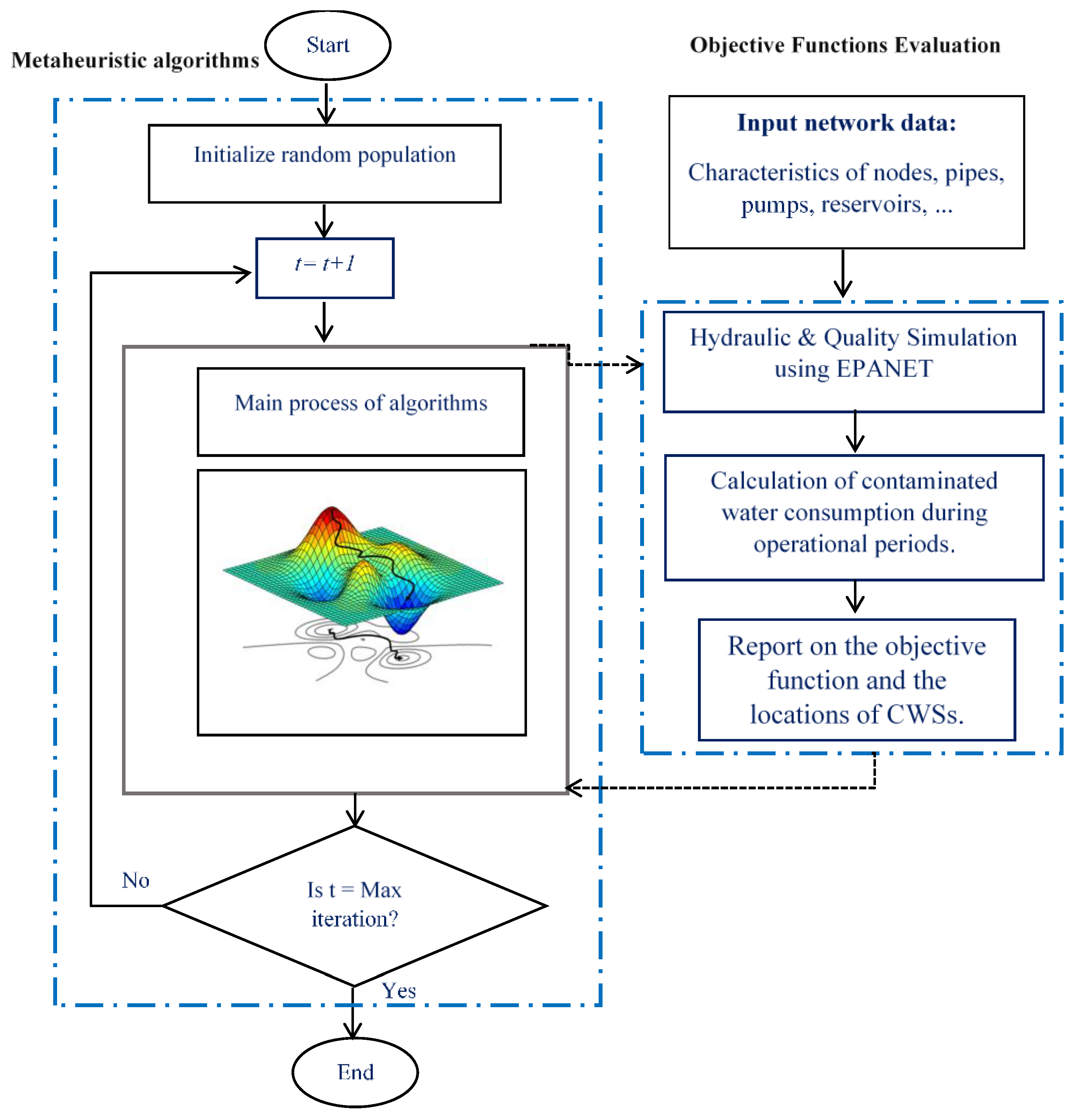
In this section, the methods used in this paper, including the qualitative simulation model of WDSs and MAs for the sustainable management of WDSs, are described. Figure 1 shows the general diagram of the optimization-simulation process developed in this work.

Figure 1.
Flowchart of the developed simulation-optimization models.
First, based on the available information for water networks (e.g., node details, pipe details, demand, etc.), these networks were modeled within the EPANET 2.2 software environment [38]. Next, using the available functions to establish a connection between MATLAB and EPANET, the two software environments were integrated. Pollution injection scenarios and alternative network demand were generated using the MATLAB 2022b software environment. The purpose of generating alternative demand, rather than relying on actual demand, is to account for uncertainty. To achieve this, 1000 new node demand series with a normal distribution based on the hourly average for each hour of the day, and a coefficient of variation of 10%, were created. Additionally, 1000 random position series were produced to represent pollution injection locations, with a rate of 10 mg/L and a duration of 2 h, reflecting the randomness of injection locations. Subsequently, by connecting EPANET to optimization algorithms within MATLAB, sensor locations were identified. In each iteration, after sensor placement, the algorithms calculated the objective function, which measured the volume of contaminated water (damage). Notably, the maximum risk calculated for each scenario (generated data series) was used as the objective function. As illustrated in Figure 1, after determining the values of the decision variables in each iteration of the optimization process, MAs were coupled with the EPANET simulator. This enabled the simulation of water quality and hydraulics to calculate the objective function and constraints. The iterative process continued until the termination condition was met. The general framework for optimizing the placement of quality sensors in networks, as used in this study, is outlined as follows:
Step 1: Generation of contamination infection scenarios based on the number of nodes and total simulation time.
Step 2: The process starts with the random generation of initial solutions, which represent the locations of CWSs within the network.
Step 3: The objective function is computed, constraints are managed, and solutions are arranged in ascending order based on objective function values. To evaluate the objective function, decision variables are first generated, and the EPANET simulator model is then used to perform both quantitative and qualitative simulations. When pollution reaches the sensors, it is assumed that no further contaminated water is consumed. The objective function, representing the volume of water, is then calculated.
Step 4: Generation of decision variables (new solutions for sensor positions) based on the theory of optimization algorithms.
Step 5: Repeat step 4 until the stopping condition of the algorithms is satisfied.
2.1. Simulation, Objective Function, and Constraints
EPANET, one of the most powerful simulation software for WDSs, was used in this study for modeling. By receiving information about nodes, valves, pumps, tanks, reservoirs, and pipes, this software calculates the quantity and direction of flow in the pipes, as well as the remaining pressure and flow rate in the nodes, according to the energy and continuity equations. The continuity and energy equations were constructed for each node and each loop, respectively, as follows [38]:
Here, denotes the count of pipes linked to node j; N represents the total number of nodes; and are the flow rate between nodes i and j, and the nodal demand at node j. In Equation (2), represents the head added by pumping stations, is the number of pipes in loop i, and represents the head loss between nodes i and j.
These two equations are interconnected through the computation of friction losses within the pipes. The Hazen–Williams equation is one of the accurate and common methods for estimating the head drop in pipes, and it is also used in this research. This equation is expressed as follows in SI units [38]:
where and are the length and diameter of pipe, respectively. is the Hazen–Williams coefficient, and represents the flow rate in pipe ij linking node i to j.
The quality simulation of WDSs in EPANET was done by using dynamic implicit approach. The flow derived from the hydraulic simulation process was applied to resolve a mass conservation equation for the substance within each pipe linking the nodes i and j as follows:
where is the rate of reaction (mass/volume/time), and and are the concentration of substance and the area of the cross-section (m2) of pipe linking nodes i, j, respectively.
It is worth mentioning that Equation (4) needs to be addressed under two specific conditions at node i: a predefined initial state at t = 0 and Equation (5) serving as the boundary condition at :
where represents the mass of the substance introduced by an external source at node i and is the corresponding source flow rate. denotes the length of pipe K that connects to node i. For further details on water quality analysis in water distribution networks, please refer to [38].
Objective Function
This research addresses the challenge of strategically positioning CWSs in WDSs by framing it as a single-objective optimization task. The goal is to reduce the network’s potential for the most severe impact-risk. Various approaches can be utilized to quantify water quality risk in WDSs, such as violations of permissible residual chlorine levels [39], assessing water quality reliability [40], minimizing water age at nodes [16], and more [41]. In this research, impact risk was quantified based on the amount of contaminated water consumed at consumer nodes.
Under the premise that contamination emanates from the k-th node at the s-th time step, the resultant risk at the j-th node during the t-th time step is quantified as follows [2,42]:
where represents the contamination concentration and indicates the water demand at the j-th node during the t-th time step.
For a more precise simulation, any concentration levels falling below the permissible threshold were assigned a value of zero to exclude them from the impact risk assessment. Additionally, the use of contaminated water persisted until detection by sensors, at which point the risk impact was nullified due to cessation of water distribution and consumption within the network. Prior to optimization, risk matrices were constructed to aid in sensor placement. Essentially, potential risk was calculated for every conceivable contamination scenario. The computation of the risk matrix proceeds as follows:
where is the risk matrix with the assumption of the inflow of contamination from the k-th node at time s. Also, nj and nt are the total number of harvesting nodes and simulation steps, respectively. Because the water quality risk reduces to zero once the sensor detects the pollution, a binary coefficient was proposed to adjust the risk calculation accordingly.
where denotes the adjusted risk, reflecting the sensors’ performance, and indicates the time step at which the first sensor in the network identifies contamination originating from the k-th node at time t. The binary parameter depends on the concentration levels and sensor placement, ensuring that the risk is assessed only prior to flow interruption. Consequently, the overall quality risk of the WDS is calculated as follows [42]:
Ultimately, the optimization challenge for CWSs in WDSs can be expressed mathematically as follows:
where is the objective function that quantifies the estimated worst-case impact risk based on the decision variables and the parameters . The decision variables represent the position of nodes recognized for locating the CWSs, which are crucial for determining the optimal configuration of the network.
Considering the increase in the complexity of the problem with the increase in the number of consumption nodes and simulation time, MAs are the best choice for solving the problem of optimizing the position of CWSs compared to gradient methods. Gradient methods, which rely heavily on derivatives and predefined initial solutions, are prone to becoming trapped in local minima. In contrast, MAs employ stochastic processes and exploration-based strategies to more effectively navigate the solution space, making them less vulnerable to the challenges posed by both linear and nonlinear optimization functions [43,44,45,46]. In the following, an overview of the algorithms used in this research is provided.
2.2. Metaheuristic Algorithms
This subsection provides a brief explanation of the optimization algorithms used in this research. It should be noted that only the important and general aspects of each algorithm are presented here. Readers can refer to the main references mentioned for more details and to learn the optimization process with these algorithms. All the optimization algorithms were developed using the MATLAB 2022b software environment, and their codes are available as open source in accordance with their original references.
2.2.1. Artemisinin Optimization (AO) Algorithm
The AO algorithm draws inspiration from artemisinin therapy for malaria, which focuses on completely eliminating malarial parasites from the human body. It comprises three optimization stages: a broad elimination phase that mimics global exploration, a localized clearance phase for targeted exploitation, and a final consolidation phase designed to improve the algorithm’s capacity to avoid being trapped in local optima [47].
2.2.2. Educational Competition Optimizer (ECO)
This algorithm is inspired by the competitive dynamics in real-world educational resource allocation scenarios. The overall process of EOA consists of three stages: elementary, middle, and high school. Based on these stages, the answers obtained in the optimization process are modified and improved [48].
2.2.3. Fata Morgana Algorithm (FATA)
FATA is modeled after the phenomenon of mirage formation, incorporating the Mirage Light Filter (MLF) principle and the Light Propagation Strategy (LPS). The MLF strategy, combined with deterministic integration, refines the algorithm’s initial solutions during the exploration phase. Subsequently, the LPS strategy, paired with trigonometric principles, guides the algorithm’s search factors into the exploitation phase, enhancing its convergence rate [35].
2.2.4. Moss Growth Optimization (MGO)
MGO is an innovative evolutionary algorithm modeled on moss growth. It begins by establishing the population’s evolutionary trajectory through a wind direction determination mechanism. Inspired by moss reproduction methods—namely, asexual, sexual, and vegetative—it employs spore dispersal search for the exploration phase and dual propagation search for the exploitation phase. Lastly, MGO incorporates a cryptobiosis mechanism, replacing traditional methods for enhancing individual solutions, which helps the algorithm avoid becoming stuck in local optima [49].
2.2.5. Parrot Optimizer (PO)
The PO algorithm draws inspiration from the observed behaviors of Pyrrhura Molinae parrots (i.e., staying, foraging, fear, and communicating) to solve continuous space optimization problems. The main optimization procedure in PO is constructed based on these behaviors to facilitate the search, finding, and improving of optimal solutions. Each search agent in this algorithm randomly follows one of the four mentioned behaviors, reflecting a more realistic definition of the random behavior of parrots in reality. This significantly reduces the probability of PO getting trapped in local optima. Unlike other metaheuristic algorithms that follow separate exploration and exploitation phases, PO integrates these behaviors seamlessly [50].
2.2.6. Polar Lights Optimizer (PLO)
PLO takes inspiration from the polar lights, or aurora, a distinctive natural event triggered by the convergence of energetic particles from the solar wind at Earth’s poles. This occurs as these particles interact with the Earth’s atmosphere and geomagnetic field, resulting in the aurora display. In this algorithm, new solutions are refined with each iteration by leveraging the motion of energetic particles and applying fundamental physics principles for exploration. First, the particles are simulated using the rotational motion model during the exploitation phase and the elliptical walking mechanism of the aurora borealis during the global exploration phase. The combination of these two strategies creates a suitable interaction between local operation and global exploration in PLO [51].
2.2.7. Rime Optimization Algorithm (RIME)
The RIME algorithm is founded on simulating the exploration and exploitation stages of metaheuristic optimization, drawing inspiration from the formation of soft-rime and hard-rime ice. Accordingly, it employs a soft-rime search strategy and a hard-rime drilling mechanism to address optimization challenges. Additionally, the algorithm enhances its greedy selection mechanism to facilitate the transition of solutions from the exploration phase to the exploitation phase [37].
2.2.8. Runge Kutta Optimization (RUN)
The RUN algorithm is based on the mathematical framework of the Runge Kutta (RK) method. It utilizes the slope variations derived from the RK method as a rational and efficient search strategy for global optimization. This approach features two dynamic phases—exploration and exploitation—to explore promising areas within the feature space and progressively advance toward the global optimum. Furthermore, an enhanced solution quality (ESQ) mechanism is implemented to prevent entrapment in local optima and accelerate convergence [36].
2.2.9. Weighted Mean of Vectors (INFO)
INFO is developed through an adaptation of the weighted mean technique. This concept is utilized to establish a robust framework and refine solution vectors via an updating rule, vector combining, and local search strategies. Within this algorithm, search agents evolve using a mean-based principle and convergence acceleration. The vector combining phase integrates the resulting vectors through the updating rule to produce a viable solution. In INFO, enhancements to the updating rule and vector combining steps were made to strengthen both exploration and exploitation capabilities. Moreover, the local search phase aids the algorithm in steering clear of low-precision solutions, thereby enhancing exploitation and convergence [29].
2.2.10. Harris Hawks Optimizer (HHO)
HHO draws inspiration from the cooperative tactics and pursuit techniques of Harris hawks. These birds work together, attacking prey from various angles to catch it off guard, employing a range of clever strategies tailored to the prey’s escape patterns. This study mathematically replicates these dynamic behaviors and patterns to construct an optimization algorithm. By simulating the shift from exploration to exploitation, inspired by the fluid dynamics of falcon chases, the algorithm avoids becoming trapped in local optima [28].
3. Case Studies
3.1. Case Study I
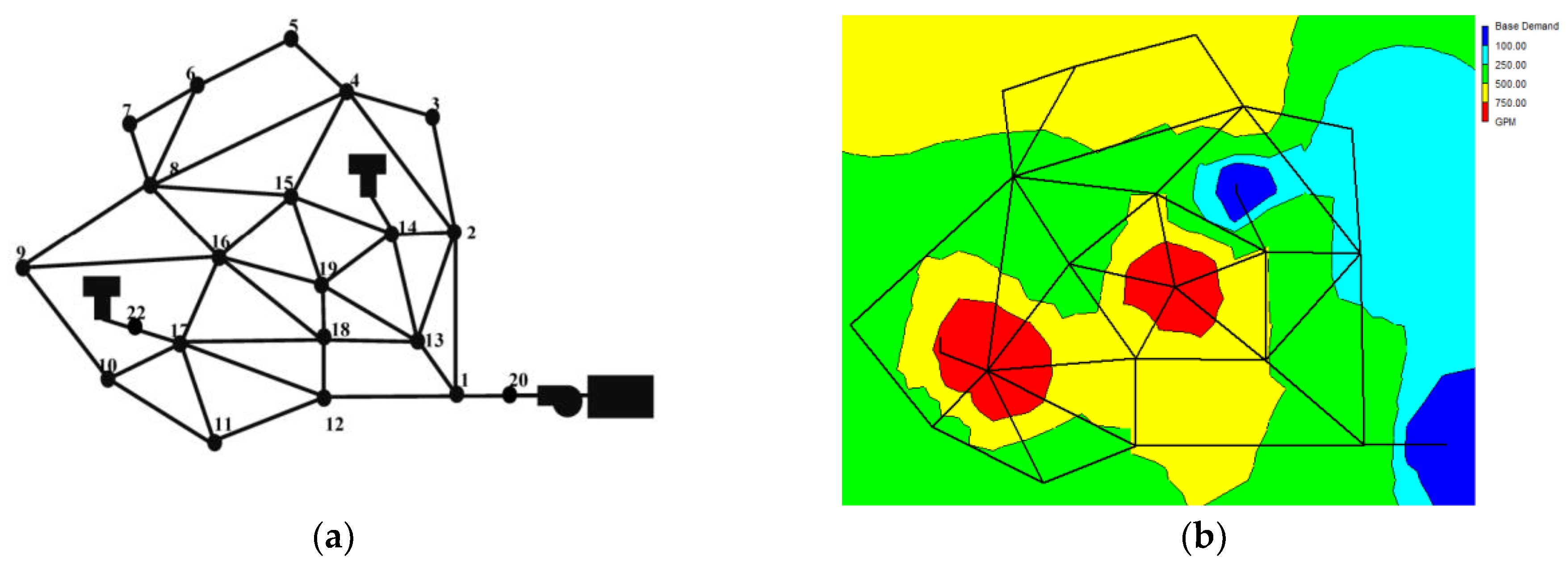
The first WDS is the Anytown network, a popular benchmark model that includes 22 nodes and 34 pipes. The water in this network is distributed directly to the nodes through a main reservoir by three pumps [2]. Additionally, a storage tank is installed in the network to supply pressure to nodes far from the pumping station. Figure 2 illustrates the layout of Anytown’s network, which has been employed in numerous studies with varying goals. (e.g., water quality management, leakage control, optimization of energy consumption, etc.). The purpose of choosing it in this study is to validate the developed codes.
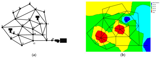
Figure 2.
Schematic of Anytown network (a) and based demands at nodes (b).
3.2. Case Study II
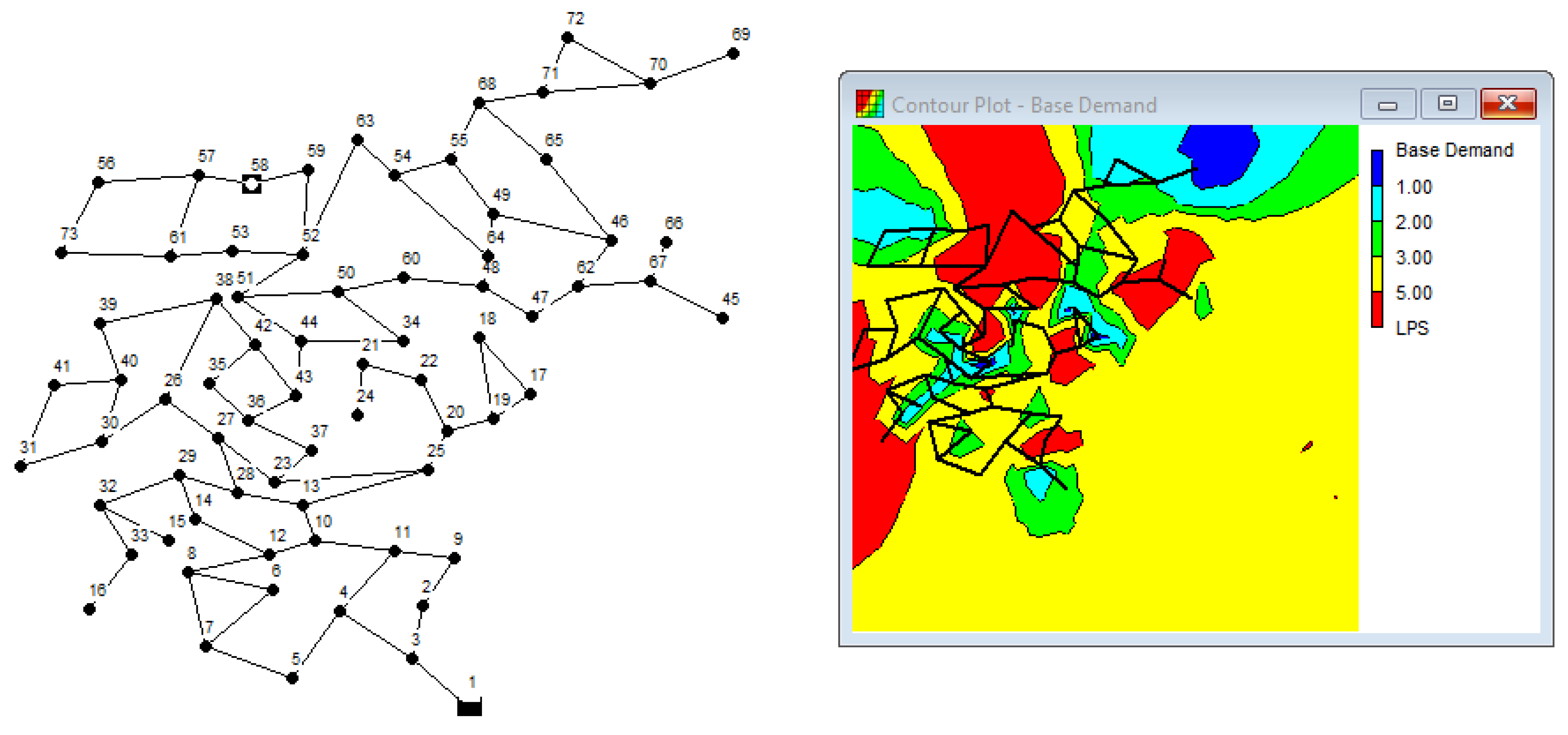
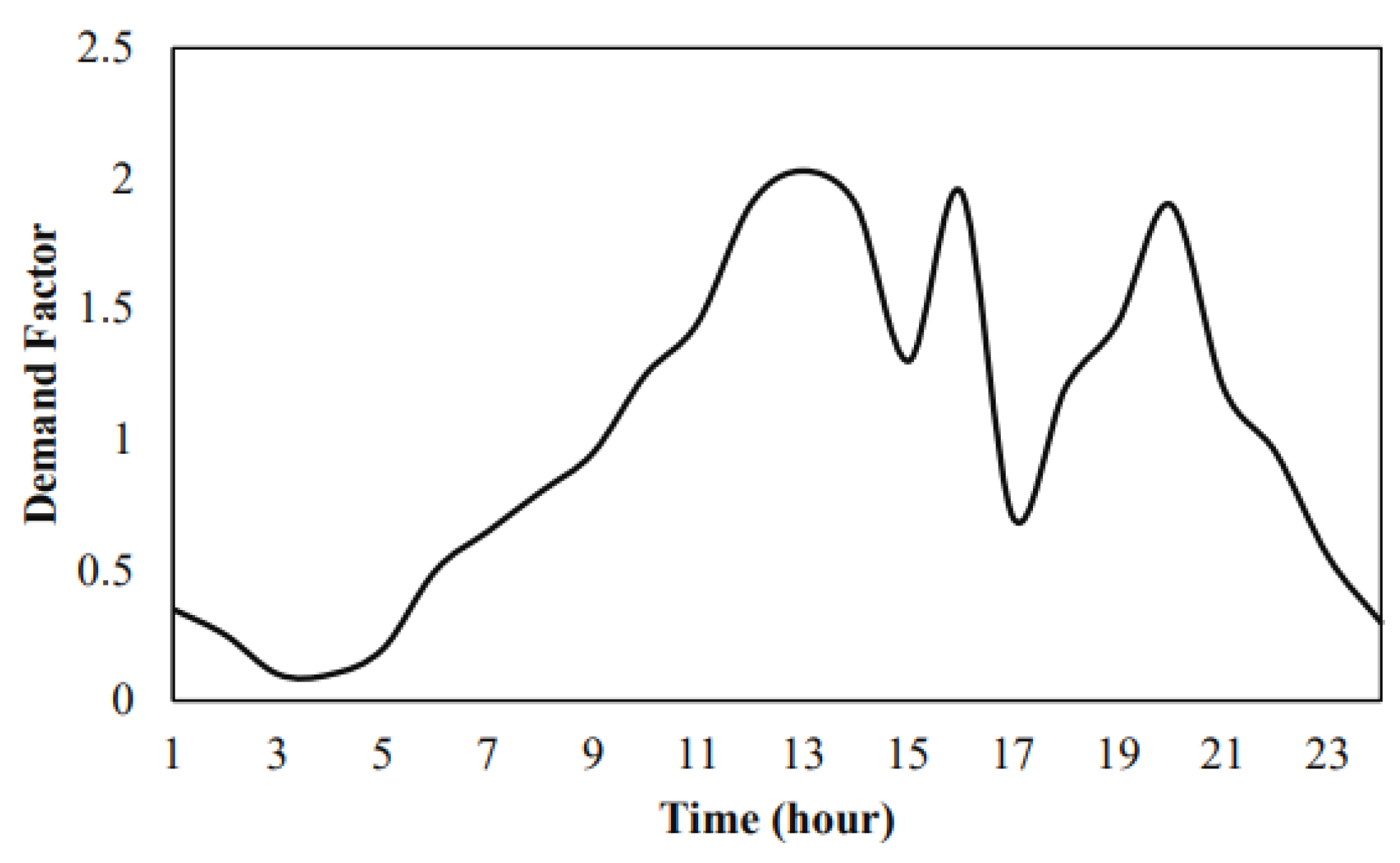
The WDS for the second case study pertains to a segment of the water network in Baghmalek City, situated in southern Iran [2,52]. This network includes 72 nodes and 90 pipes made of polyethylene with a Hazen–William’s coefficient of 130. A major concern is the demand of the nodes and the pressure on the network. Due to the region’s high soil salinity and close proximity to oil reserves, there is a considerable risk of chemical contamination in the WDS caused by negative pressure. To mitigate this risk, enhancing water quality reliability through the optimal positioning of CWSs is essential. The schematic of the Baghmalek network is presented in Figure 3. Additionally, the network demand coefficient for a 24 h period is shown in Figure 4. As is known, the peak consumption time in the network is at 13:00, and the lowest consumption occurs between 2:00 and 5:00 a.m.
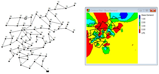
Figure 3.
Schematic of Baghmalek WDS.
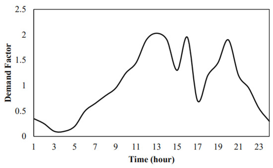
Figure 4.
Coefficients of consumption in Baghmalek WDS.
4. Results and Discussion
4.1. General Setting of the Algorithm
Each MA has a series of fixed or dynamic parameters that need to be determined before use. Different methods are employed for this purpose, with sensitivity analysis being one of the most common methods based on trial and error. Although this approach is suitable, it is very time-consuming. According to research conducted by Arcuri and Fraser [53], the optimal parameter values for MAs in solving different problems are those recommended in their primary references. Accordingly, Table 2 presents the parameter settings for each algorithm based on these references. To ensure a fair comparison, each algorithm was run 30 times, with 1000 iterations and an initial population of 50.
Table 2.
Optimal values for the metaheuristic algorithm’s parameters.
4.2. Results of Case Study I
After setting the parameters of the algorithms, all the algorithms were executed 20 times for the optimal placement of four CWSs in the Anytown network. Notably, in previous research conducted on this network [2,54], the number of CWSs was set to four. To facilitate comparison between the results of this study and prior research, as well as to validate the findings, the number of sensors in this study was also set to four. As noted, the criteria for comparing algorithms in this study are limited to the magnitude of the objective function obtained and their convergence speed. Given the similar nature of these algorithms, their computational time showed minimal variation. Therefore, the focus of this research has been exclusively on evaluating the accuracy of the algorithms. Table 3 presents the probabilistic analysis of the solutions obtained from the algorithms for 20 executions, which includes the average, standard deviation (SD), best (minimum), and worst (maximum).
Table 3.
Results of algorithms on case study I.
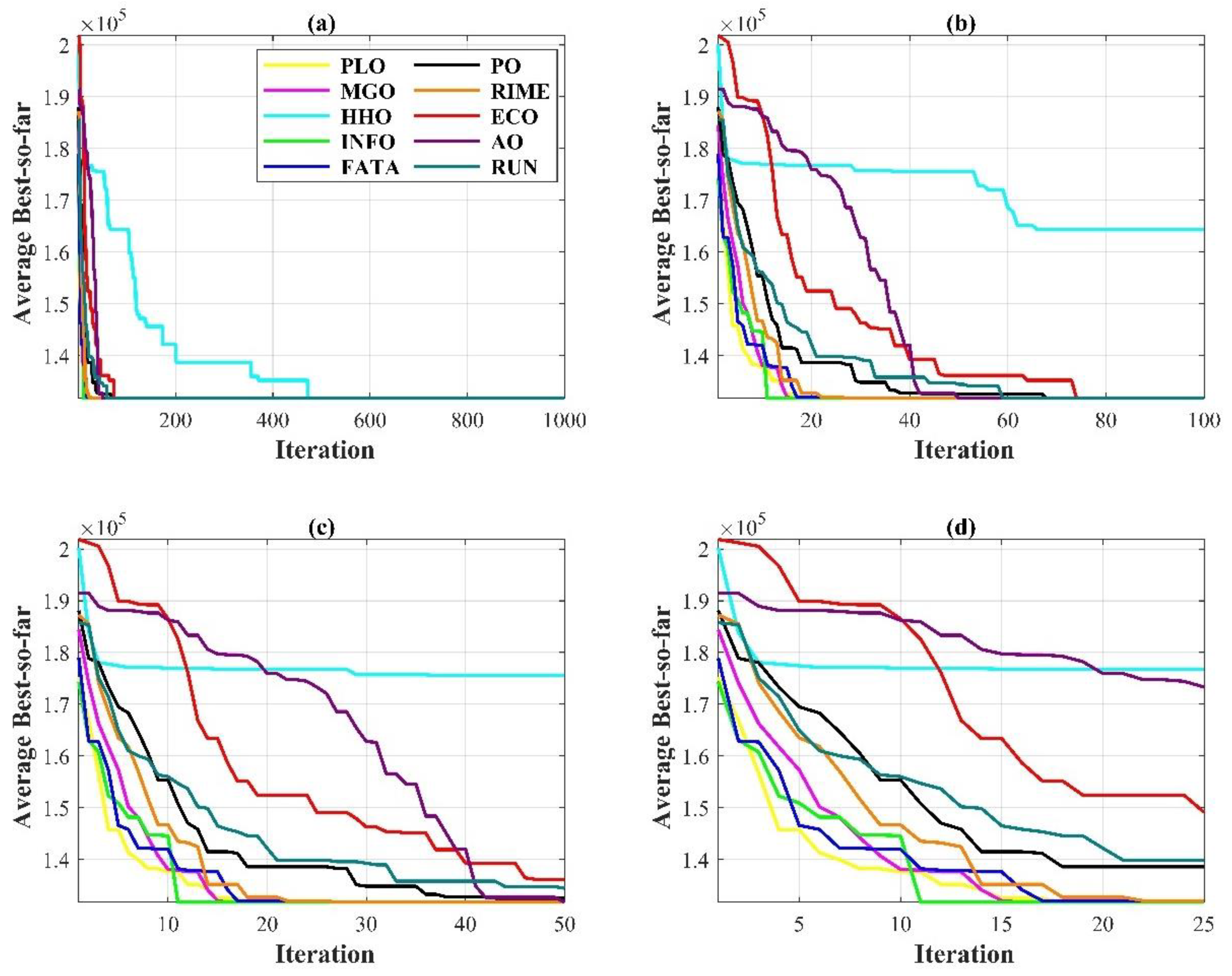
As illustrated in Table 2, all 10 algorithms successfully achieved the optimal solution of 131,754 m3 across 20 executions. Interestingly, the worst, best, average, and standard deviation values remained identical. This outcome is attributed to the randomized yet closely related nature of these algorithms, leading them to converge on the same solution. Beyond the quantitative assessment of the objective function, an essential criterion for evaluating algorithm performance is convergence rate. Specifically, an algorithm that reaches the optimal solution in fewer iterations (with minimal objective function evaluations) demonstrates superior convergence efficiency. In Figure 5a, the average convergence curve of the algorithms for the Anytown network is presented. As shown, all the algorithms except HHO converged within 100 iterations and were able to provide the optimal solution of 131,754 m3. HHO converged in iteration 471. Consequently, from the perspective of convergence, it had the worst performance compared to the other nine algorithms. Figure 5b–d show more details of the convergence of the algorithms. INFO performed best, with an average convergence in 11 iterations. MGO and PLO both converged in 15 iterations. FATA and RIMA converged in 16 and 21 iterations, respectively; AO in 50 iterations; Run in 59 iterations; and ECO in 74 iterations.
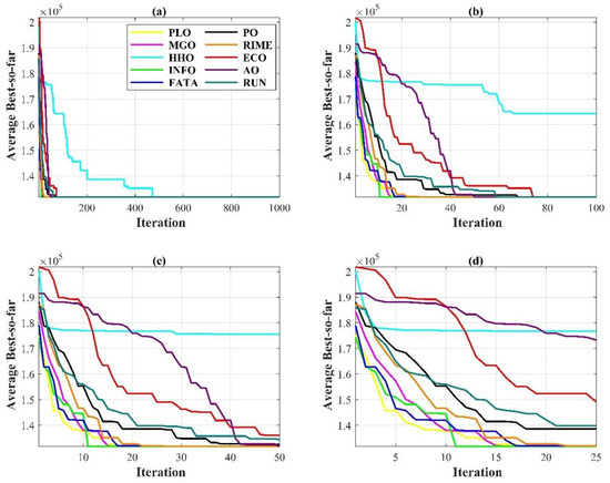
Figure 5.
Convergence curve of algorithms for Anytown network; (a) convergence in 1000 iterations; (b) convergence in 100 iterations; (c) convergence in 50 iterations; and (d) convergence in 25 iterations.
Eliades et al. (2014) used this network to evaluate their proposed S-PLACE toolkit-based genetic algorithm (GA) for placement CWSs [54]. They managed to reduce the amount of polluted water to 138,808 m3 by using the optimal placement of four CWSs. Furthermore, Ahmedabadi et al. [2] reduced the volume of contaminated water to 131,754 m3 by combining the whale optimization algorithm (WOA) [55] and sand cat swarm optimization (SCSO) [56]. In Table 4, the results presented in Ahmedabadi et al.’s [2] research are reported as the average of 10 executions of different algorithms. As shown, the hybrid WOA-SCSO algorithm performed better compared to the WOA, simulated annealing-based WOA (WOA-SA), dragonfly algorithm (DA) [57], moth–flame optimization (MFO) [58], and SCSO algorithms, providing the lowest value of the objective function (the volume of polluted water consumed).
Table 4.
Results of [2] study on Anytown network.
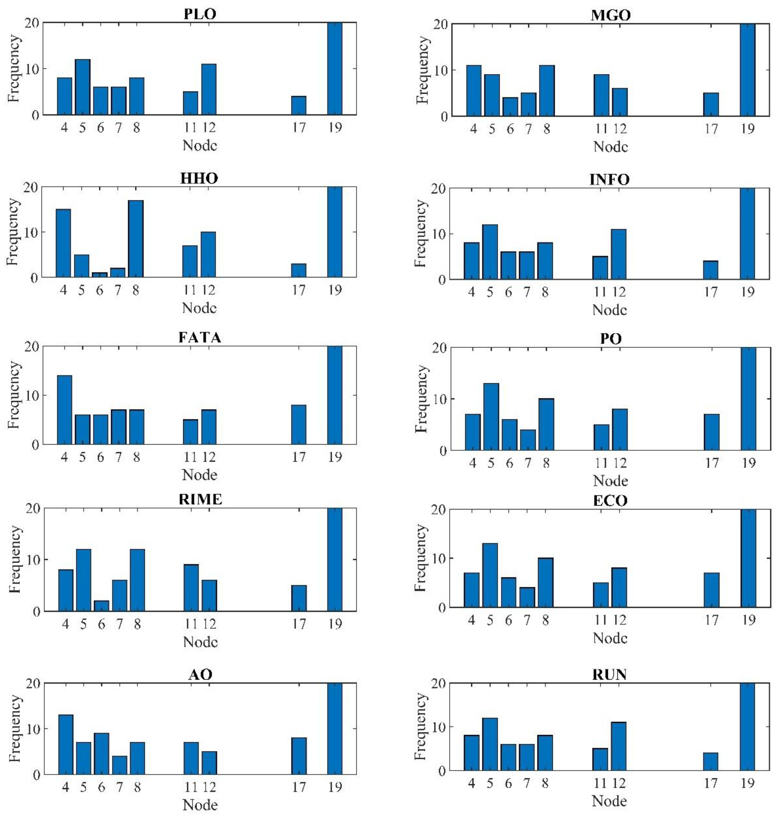
Comparing the solutions obtained from the algorithms used in this research with the older algorithms (i.e., WOA, SCSO, WOA-SA, MFO, and DO) used in the research of Ahmadabadi et al. [2] shows that the recently proposed algorithms provide better answers than the previous algorithms. As shown, among the algorithms analyzed in the study by Ahmadabadi et al. [2], only one hybrid algorithm achieved an optimal solution comparable to the algorithms employed in this research. This is attributed to the fact that the other algorithms are classical, while WOA-SCSO represents a novel hybrid algorithm. In Figure 6, the frequency of the optimal nodes selected for the installation location of the CWSs by the algorithms is presented. As shown, nodes 4, 5, 6, 7, 8, 11, 12, 17, and 19 were identified as the best locations in 20 executions of all algorithms for installing CWSs. Node 19, which had the highest base demand in the network, can be introduced as the most important node and a strategic position for placing CWSs to minimize damage. It is noteworthy that in some algorithms, the frequency of solutions is similar, indicating that the main structure of these algorithms is similar to each other.

Figure 6.
Frequency of obtained solutions by algorithms.
4.3. Results of Case Study II
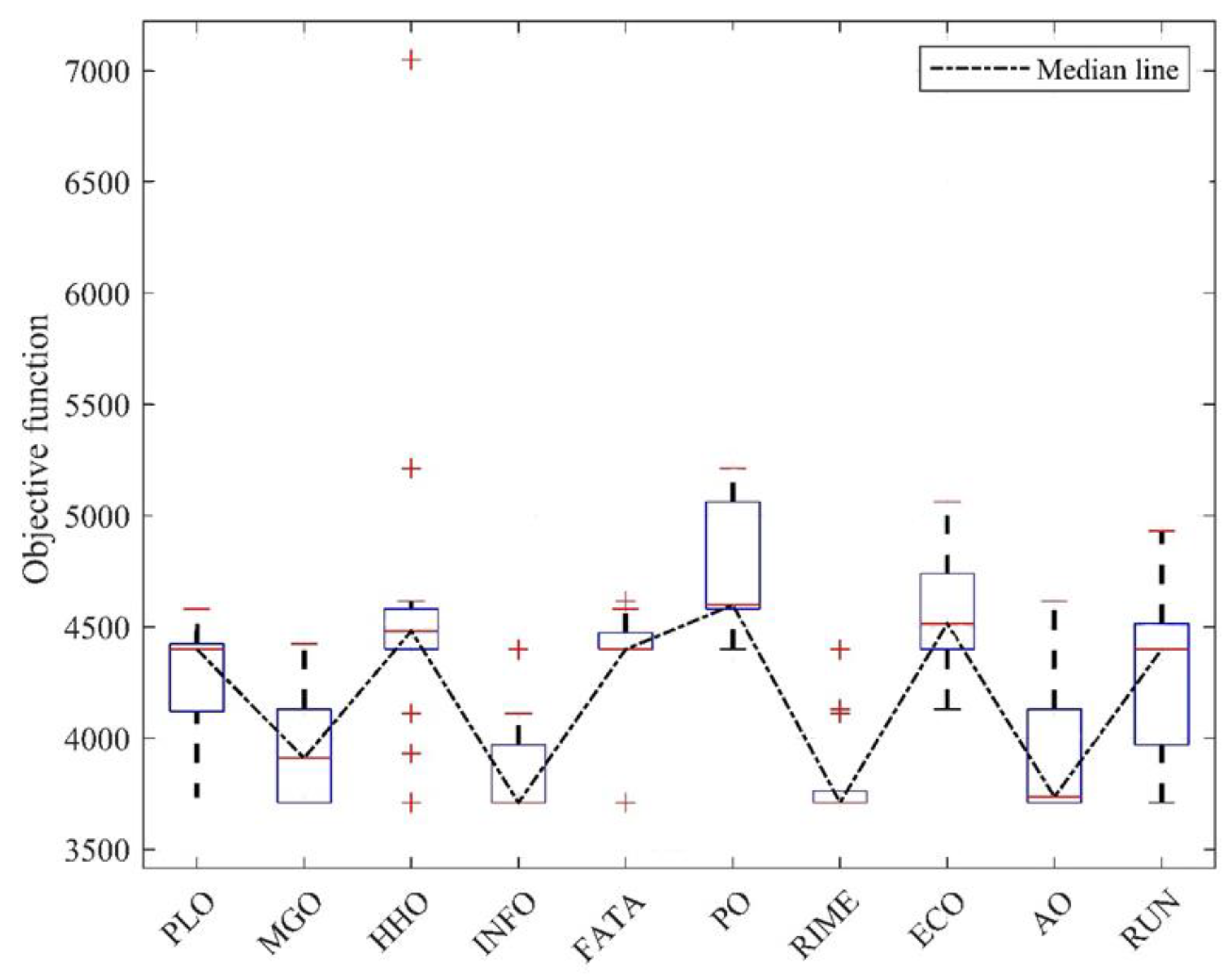
According to the previous subsection, each algorithm for the second case study was run 20 times with an initial population of 50 and 1000 iterations. Table 5 provides an analysis of the solutions obtained from these implementations, considering 10 CWSs. The lowest average value and standard deviation of the responses obtained for RIME in reducing the risk of consuming contaminated water in the Baghmalek WDS were achieved with the optimal placement of the sensors in 20 executions of the algorithm. The average and standard deviation of the responses for this algorithm were 3.8133 × 10³ L and 2.0093 × 10² L, respectively. Additionally, the minimum and maximum values of the objective function calculated by RIMA were 3.7100 × 10³ L and 4.3989 × 10³ L, respectively. After RIME, the INFO and MGO algorithms performed better than other algorithms in terms of average and standard deviation of responses. To show the range and deviation from the criteria of the responses obtained by the algorithms, a box plot diagram is presented in Figure 7 for all the algorithms.
Table 5.
Results of algorithms on case study II.
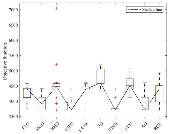
Figure 7.
Box plot of algorithm performance.
As shown in Figure 7, HHO had the largest standard of deviation, equal to 6.7592 × 10² L, which does indicate the algorithm’s weakness in examining the mentioned problem. Additionally, the worst average solution belonged to the PO algorithm, equal to 4.7842 × 10³ L. The range of responses is clearly visible in Figure 4. Furthermore, the median line, which indicates the tendency of the data to be higher or lower than the average, is shown in this figure. According to Figure 4, it can be said that the ECO and AO algorithms, with a higher median line in the box, had a higher average performance than the PLO and MGO algorithms, which had a lower median line in the box. It is also evident that RIME and FATA had skewed data distributions because the median line was not centered. In fact, the median line represents the central tendency of the data.
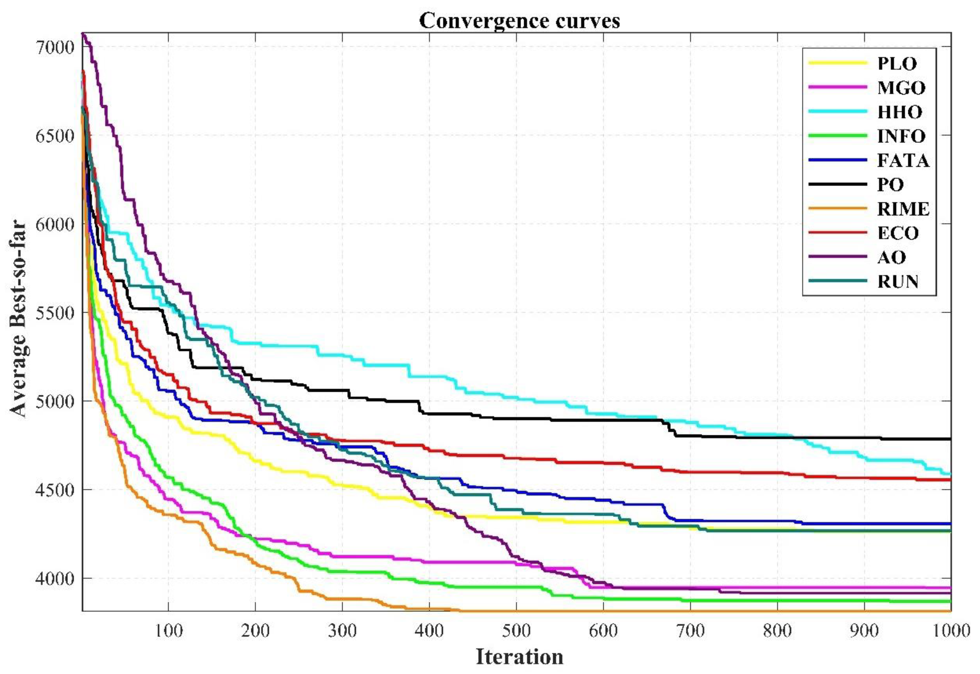
The convergence curve of the algorithms for the second water network is presented in Figure 8. As shown, RIME converged in earlier iterations than other algorithms, resulting in the lowest value of the objective function. INFO and MGO algorithms followed, with lower convergence rates compared to other algorithms. PO had a higher convergence rate, converging later than other algorithms and providing the worst average. HHO also converged later, but ultimately gave the same solution as ECO, with the difference that ECO converged in fewer than 50 iterations. A noteworthy point is that the algorithms in solving the first case study reached the solution in the initial iterations. However, to solve the second network, which was larger than the first, they searched for the optimal solution until the final iterations. This was because, with the increase in the number of network nodes, the complexity of the problem increased, enlarging the search space and requiring the algorithms to search more extensively.
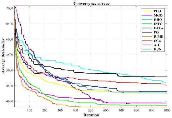
Figure 8.
Average convergence curves of algorithms for case study II.
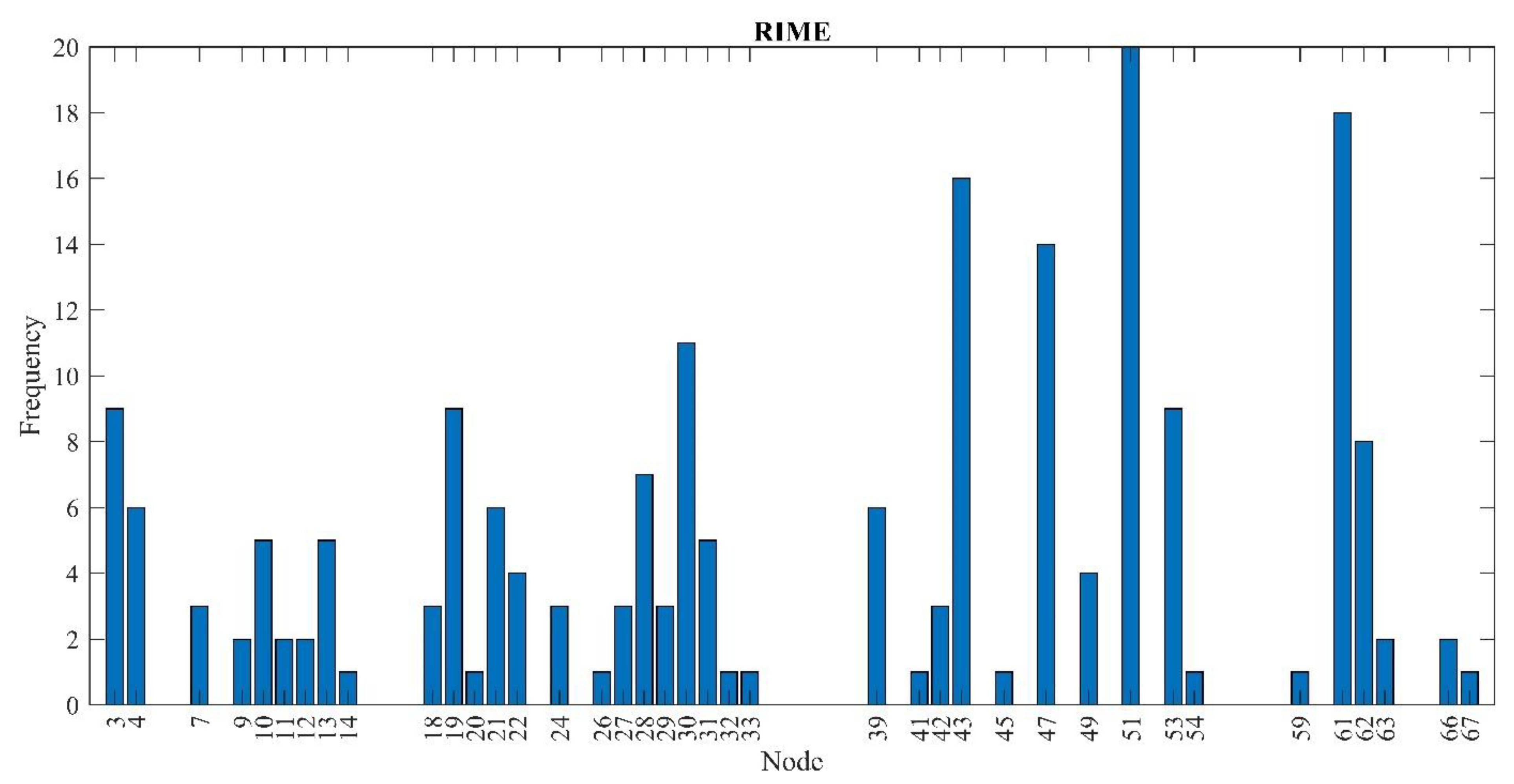
Previously, Ahmedabadi et al. [2] estimated the value of the objective function (contaminated water consumed) by placing 10 sensors in nodes 53, 31, 33, 19, 51, 45, 37, 9, 36, and 47, using the WOA-SCSO hybrid algorithm, reducing it to 4855 L. Comparing the results of this study demonstrates that the recently proposed algorithms outperformed both the classic and hybrid algorithms in addressing the problem of optimal placement of CWSs within WDSs. The frequency of obtained solutions (nodes selected to install CWSs) by RIME is presented in Figure 9. As can be seen, nodes 51, 61, and 43 were identified as the most effective CWS placement points in the Baghmalek network, with 20, 18, and 17 selections, respectively, in 20 executions of the algorithm. In reference to the previous example, the study results indicate that the most optimal locations for installing CWSs within the network were nodes with the highest demand, as these points experienced the greatest water consumption. As outlined in Equation (6), the volume of contaminated water consumed was directly influenced by nodal demand and pollutant concentration. However, further extensive research is necessary to substantiate this claim.
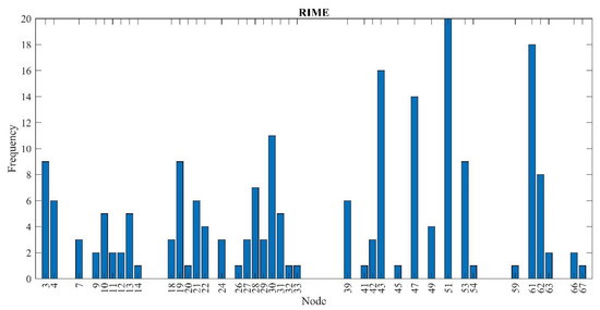
Figure 9.
Frequency of selected nodes for placement CWSs in the Baghmalek network.
5. Conclusions
In this study, the accuracy and computational efficiency of ten metaheuristic algorithms for the optimal placement of CWSs in WDSs were evaluated using both a benchmark network and a real-world network. To achieve this, the optimal placement problem for CWSs in WDSs was formulated as a single-objective optimization problem within the MATLAB software environment, dynamically integrated with the EPANET simulator. The objective function aimed to minimize the volume of contaminated water consumed. In the benchmark water network, the algorithms successfully converged in fewer than 500 iterations and identified the optimal solution. The INFO with the lowest convergence rate of 11 iterations demonstrated the best performance among all algorithms. Following INFO, MGO and PLO both achieved a convergence rate of 15 iterations, while FATA and RIMA recorded convergence rates of 16 and 21 iterations, respectively. AO exhibited a convergence rate of 50 iterations, RUN had a rate of 59 iterations, PO reached 69 iterations, and ECO showed a rate of 74 iterations. Finally, HHO, with the highest convergence rate of 471 iterations, delivered the most favorable objective function value.
In the second case study, where the network was larger, the solution space became broader and more complex. The algorithms continued to explore the decision space until the final iteration. Consequently, in the second network, the RIME algorithm achieved the lowest objective function value in fewer than 500 iterations, representing the lowest convergence rate for the best objective function value among the 10 algorithms examined.
Overall, the INFO algorithm provided the best solutions in the first case, while the RIME algorithm performed best in the second case, delivering optimal results in the fewest iterations. Among the algorithms, HHO exhibited a higher convergence rate compared to the others, with more favorable range, standard deviation, and mean values in the solutions obtained.
For future work, it is recommended to formulate the CWS placement problem as a multi-objective optimization problem and address it using multi-objective versions of the algorithms employed in the present study, along with NSGA-II. Additionally, combining these algorithms to enhance their performance could be explored. Furthermore, it is proposed to conduct a dedicated study on the sensitivity analysis of the optimization algorithm parameters, examining the impact of their variations on the objective function value in the context of the current problem.
Author Contributions
Conceptualization, J.J.-A.; Methodology, S.A.S.S., Z.A. and A.B.M.; Software, S.A.S.S., Z.A. and J.J.-A.; Validation, Z.A. and A.B.M.; Investigation, S.A.S.S. and J.J.-A.; Writing—original draft, S.A.S.S., Z.A. and A.B.M.; Writing—review & editing, J.J.-A. All authors have read and agreed to the published version of the manuscript.
Funding
This research received no external funding.
Data Availability Statement
The data presented in this study are available on request from the corresponding author.
Conflicts of Interest
The authors declare no conflict of interest.
References
- Berry, J.; Hart, W.E.; Phillips, C.A.; Uber, J.G.; Watson, J.-P. Sensor placement in municipal water networks with temporal integer programming models. J. Water Resour. Plan. Manag. 2006, 132, 218–224. [Google Scholar] [CrossRef]
- Afzali Ahmadabadi, S.; Jafari-Asl, J.; Banifakhr, E.; Houssein, E.H.; Ben Seghier, M.E.A. Risk-Based Design Optimization of Contamination Detection Sensors in Water Distribution Systems: Application of an Improved Whale Optimization Algorithm. Water 2023, 15, 2217. [Google Scholar] [CrossRef]
- Weickgenannt, M.; Kapelan, Z.; Blokker, M.; Savic, D.A. Risk-based sensor placement for contaminant detection in water distribution systems. J. Water Resour. Plan. Manag. 2010, 136, 629–636. [Google Scholar] [CrossRef]
- Lee, B.H.; Deininger, R.A. Optimal locations of monitoring stations in water distribution system. J. Environ. Eng. 1992, 118, 4–16. [Google Scholar] [CrossRef]
- Kessler, A.; Ostfeld, A. Detecting accidental contaminations in municipal water networks: Application. In Proceedings of the Annual Water Resources Planning and Management Conference, Chicago, IL, USA, 8–10 June 1998. [Google Scholar]
- Kessler, A.; Ostfeld, A.; Sinai, G. Detecting accidental contaminations in municipal water networks. J. Water Resour. Plan. Manag. 1998, 124, 192–198. [Google Scholar] [CrossRef]
- Harmant, P.; Nace, A.; Kiene, L.; Fotoohi, F. Optimal supervision of drinking water distribution network. In WRPMD’99: Preparing for the 21st Century; Amer Society of Civil Engineers: Reston, VA, USA, 1999; pp. 1–9. [Google Scholar]
- Al-Zahrani, M.A.; Moeid, K. Locating optimum water quality monitoring stations in water distribution system. In Proceedings of the Bridging the Gap: Meeting the World’s Water and Environmental Resources Challenges—Proceedings of the World Water and Environmental Resources Congress 2001, Orlando, FL, USA, 20–24 May 2001; Volume 111. [Google Scholar] [CrossRef]
- Afshar, A.; Mariño, M.A. Multi-objective coverage-based ACO model for quality monitoring in large water networks. Water Resour. Manag. 2012, 26, 2159–2176. [Google Scholar] [CrossRef]
- Aral, M.M.; Guan, J.; Maslia, M.L. Optimal design of sensor placement in water distribution networks. J. Water Resour. Plan. Manag. 2010, 136, 5–18. [Google Scholar] [CrossRef]
- Kim, J.H.; Tran, T.V.T.; Chung, G. Optimization of water quality sensor locations in water distribution systems considering imperfect mixing. In Water Distribution Systems Analysis 2010; American Society of Civil Engineers: Reston, VA, USA, 2010; pp. 317–326. [Google Scholar]
- Bazargan-Lari, M.R.; Taghipour, S.; Habibi, M. Real-time contamination zoning in water distribution networks for contamination emergencies: A case study. Environ. Monit. Assess. 2021, 193, 336. [Google Scholar] [CrossRef]
- Afshar, A.; Miri Khombi, S.M. Multiobjective optimization of sensor placement in water distribution networks dual use benefit approach. Iran Univ. Sci. Technol. 2015, 5, 315–331. [Google Scholar]
- Naserizade, S.S.; Nikoo, M.R.; Montaseri, H.; Alizadeh, M.R. A Hybrid Fuzzy-Probabilistic Bargaining Approach for Multi-objective Optimization of Contamination Warning Sensors in Water Distribution Systems. Group Decis. Negot. 2021, 30, 641–663. [Google Scholar] [CrossRef]
- Shoorangiz, M.; Nikoo, M.R.; Šimůnek, J.; Gandomi, A.H.; Adamowski, J.F.; Al-Wardy, M. Multi-objective optimization of hydrant flushing in a water distribution system using a fast hybrid technique. J. Environ. Manag. 2023, 334, 117463. [Google Scholar] [CrossRef]
- Jafari-Asl, J.; Hashemi Monfared, S.A.; Abolfathi, S. Reducing Water Conveyance Footprint through an Advanced Optimization Framework. Water 2024, 16, 874. [Google Scholar] [CrossRef]
- Storn, R.; Price, K. Differential Evolution—A Simple and Efficient Adaptive Scheme for Global Optimization over Continuous Spaces; 1995. Available online: https://link.springer.com/article/10.1023/A:1008202821328 (accessed on 27 February 2025).
- Holland, J.H. Adaptation in Natural and Artificial Systems; University of Michigan Press: Ann Arbor, MI, USA, 1975; p. 1. [Google Scholar]
- Rechenberg, I. Cybernetic solution path of an experimental problem (kybernetische lösungsansteuerung einer experimentellen forschungsaufgabe). In Evolutionary Computation: The Fossil Record; IEEE: Piscataway, NJ, USA, 1998. [Google Scholar] [CrossRef]
- Kennedy, J.; Eberhart, R. Particle swarm optimization. In Proceedings of the ICNN’95-International Conference on Neural Networks, Perth, WA, Australia, 27 November–1 December 1995; IEEE: Piscataway, NJ, USA, 1995; Volume 4, pp. 1942–1948. [Google Scholar]
- Dorigo, M.; Blum, C. Ant colony optimization theory: A survey. Theor. Comput. Sci. 2005, 344, 243–278. [Google Scholar] [CrossRef]
- Karaboga, D.; Akay, B. A comparative study of Artificial Bee Colony algorithm. Appl. Math. Comput. 2009, 214, 108–132. [Google Scholar] [CrossRef]
- Yang, X.S.; Deb, S. Cuckoo search via Lévy flights. In Proceedings of the 2009 World Congress on Nature and Biologically Inspired Computing, NABIC 2009—Proceedings, Coimbatore, India, 9–11 December 2009. [Google Scholar] [CrossRef]
- Fister, I.; Yang, X.S.; Brest, J. A comprehensive review of firefly algorithms. Swarm Evol. Comput. 2013, 13, 34–46. [Google Scholar] [CrossRef]
- Yang, X.S. A new metaheuristic Bat-inspired Algorithm. In Nature Inspired Cooperative Strategies for Optimization (NICSO 2010); Studies in Computational Intelligence; Springer: Berlin/Heidelberg, Germany, 2010; Volume 284. [Google Scholar] [CrossRef]
- Mirjalili, S.; Mirjalili, S.M.; Lewis, A. Grey Wolf Optimizer. Adv. Eng. Softw. 2014, 69, 46–61. [Google Scholar] [CrossRef]
- Mirjalili, S. Dragonfly algorithm: A new meta-heuristic optimization technique for solving single-objective, discrete, and multi-objective problems. Neural Comput. Appl. 2016, 27, 1053–1073. [Google Scholar] [CrossRef]
- Heidari, A.A.; Mirjalili, S.; Faris, H.; Aljarah, I.; Mafarja, M.; Chen, H. Harris hawks optimization: Algorithm and applications. Future Gener. Comput. Syst. 2019, 97, 849–872. [Google Scholar] [CrossRef]
- Ahmadianfar, I.; Heidari, A.A.; Noshadian, S.; Chen, H.; Gandomi, A.H. INFO: An efficient optimization algorithm based on weighted mean of vectors. Expert Syst. Appl. 2022, 195, 116516. [Google Scholar] [CrossRef]
- Kirkpatrick, S.; Gelatt, C.D.; Vecchi, M.P. Optimization by simulated annealing. Science 1983, 220, 671–680. [Google Scholar] [CrossRef]
- Deeb, H.; Sarangi, A.; Mishra, D.; Sarangi, S.K. Improved Black Hole optimization algorithm for data clustering. J. King Saud Univ.-Comput. Inf. Sci. 2022, 34, 5020–5029. [Google Scholar] [CrossRef]
- Tabari, A.; Ahmad, A. A new optimization method: Electro-Search algorithm. Comput. Chem. Eng. 2017, 103, 1–11. [Google Scholar] [CrossRef]
- Mohanty, D.K. Gravitational search algorithm for economic optimization design of a shell and tube heat exchanger. Appl. Therm. Eng. 2016, 107, 184–193. [Google Scholar] [CrossRef]
- Zhao, W.; Wang, L.; Zhang, Z. Atom search optimization and its application to solve a hydrogeologic parameter estimation problem. Knowl. Based Syst. 2019, 163, 283–304. [Google Scholar] [CrossRef]
- Qi, A.; Zhao, D.; Heidari, A.A.; Liu, L.; Chen, Y.; Chen, H. FATA: An efficient optimization method based on geophysics. Neurocomputing 2024, 607, 128289. [Google Scholar] [CrossRef]
- Ahmadianfar, I.; Heidari, A.A.; Gandomi, A.H.; Chu, X.; Chen, H. RUN beyond the metaphor: An efficient optimization algorithm based on Runge Kutta method. Expert. Syst. Appl. 2021, 181, 115079. [Google Scholar] [CrossRef]
- Su, H.; Zhao, D.; Heidari, A.A.; Liu, L.; Zhang, X.; Mafarja, M.; Chen, H. RIME: A physics-based optimization. Neurocomputing 2023, 532, 183–214. [Google Scholar] [CrossRef]
- Rossman, L. EPANET 2 User Manual. Soc. Stud. Sci. 2018, 38. Available online: https://www.microimages.com/documentation/tutorials/epanet2usermanual.pdf (accessed on 27 February 2025).
- Li, R.A.; McDonald, J.A.; Sathasivan, A.; Khan, S.J. A multivariate Bayesian network analysis of water quality factors influencing trihalomethanes formation in drinking water distribution systems. Water Res. 2021, 190, 116712. [Google Scholar] [CrossRef]
- Latifi, M.; Gheibi, M.A.; Naeeni, S.T. Improving Consumer Satisfaction in Water Distribution Networks Through Optimal Use of Auxiliary Tanks (A Case Study of Kashan City, Iran). Water Resour. Manag. 2018, 32, 4103–4122. [Google Scholar] [CrossRef]
- Gheisi, A.; Forsyth, M.; Naser, G. Water Distribution Systems Reliability: A Review of Research Literature. J. Water Resour. Plan. Manag. 2016, 142, 04016047. [Google Scholar] [CrossRef]
- Geranmehr, M.; Yousefi-Khoraem, M. Optimal Quality Sensor Placement in Water Distribution Networks under Temporal and Spatial Uncertain Contamination. J. Water Wastewater 2020, 31, 143–155. (In Persian) [Google Scholar]
- Dogani, A.; Dourandish, A.; Ghorbani, M.; Shahbazbegian, M.R. A Hybrid Meta-Heuristic for a Bi-Objective Stochastic Optimization of Urban Water Supply System. IEEE Access 2020, 8, 135829–135843. [Google Scholar] [CrossRef]
- Lee, H.M.; Jung, D.; Sadollah, A.; Lee, E.H.; Kim, J.H. Performance comparison of metaheuristic optimization algorithms using water distribution system design benchmarks. In Harmony Search and Nature Inspired Optimization Algorithms: Theory and Applications, ICHSA 2018; Advances in Intelligent Systems and Computing; Springer: Singapore, 2019; Volume 741. [Google Scholar] [CrossRef]
- El-Ghandour, H.A.; Elbeltagi, E. Comparison of Five Evolutionary Algorithms for Optimization of Water Distribution Networks. J. Comput. Civ. Eng. 2018, 32, 04017066. [Google Scholar] [CrossRef]
- Kumar, V.; Yadav, S.M. A state-of-the-Art review of heuristic and metaheuristic optimization techniques for the management of water resources. Water Supply 2022, 22, 3702–3728. [Google Scholar] [CrossRef]
- Yuan, C.; Zhao, D.; Heidari, A.A.; Liu, L.; Chen, Y.; Wu, Z.; Chen, H. Artemisinin optimization based on malaria therapy: Algorithm and applications to medical image segmentation. Displays 2024, 84, 102740. [Google Scholar] [CrossRef]
- Lian, J.; Zhu, T.; Ma, L.; Wu, X.; Heidari, A.A.; Chen, Y.; Chen, H.; Hui, G. The educational competition optimizer. Int. J. Syst. Sci. 2024, 55, 3185–3222. [Google Scholar] [CrossRef]
- Zheng, B.; Chen, Y.; Wang, C.; Heidari, A.A.; Liu, L.; Chen, H. The moss growth optimization (MGO): Concepts and performance. J. Comput. Des. Eng. 2024, 11, 184–221. [Google Scholar] [CrossRef]
- Lian, J.; Hui, G.; Ma, L.; Zhu, T.; Wu, X.; Heidari, A.A.; Chen, Y.; Chen, H. Parrot optimizer: Algorithm and applications to medical problems. Comput. Biol. Med. 2024, 172, 108064. [Google Scholar] [CrossRef]
- Yuan, C.; Zhao, D.; Heidari, A.A.; Liu, L.; Chen, Y.; Chen, H. Polar lights optimizer: Algorithm and applications in image segmentation and feature selection. Neurocomputing 2024, 607, 128427. [Google Scholar] [CrossRef]
- Minaei, A.; Haghighi, A.; Ghafouri, H.R. Computer-aided decision-making model for multiphase upgrading of aged water distribution mains. J. Water Resour. Plan. Manag. 2019, 145, 04019008. [Google Scholar] [CrossRef]
- Arcuri, A.; Fraser, G. Parameter tuning or default values? An empirical investigation in search-based software engineering. Empir. Softw. Eng. 2013, 18, 594–623. [Google Scholar] [CrossRef]
- Eliades, D.G.; Kyriakou, M.; Polycarpou, M.M. Sensor placement in water distribution systems using the S-PLACE Toolkit. Procedia Eng. 2014, 70, 602–611. [Google Scholar] [CrossRef]
- Mirjalili, S.; Lewis, A. The whale optimization algorithm. Adv. Eng. Softw. 2016, 95, 51–67. [Google Scholar] [CrossRef]
- Seyyedabbasi, A.; Kiani, F. Sand Cat swarm optimization: A nature-inspired algorithm to solve global optimization problems. Eng. Comput. 2022, 39, 2627–2651. [Google Scholar] [CrossRef]
- Meraihi, Y.; Ramdane-Cherif, A.; Acheli, D.; Mahseur, M. Dragonfly algorithm: A comprehensive review and applications. Neural Comput. Appl. 2020, 32, 16625–16646. [Google Scholar] [CrossRef]
- Mirjalili, S. Moth-flame optimization algorithm: A novel nature-inspired heuristic paradigm. Knowl. Based Syst. 2015, 89, 228–249. [Google Scholar] [CrossRef]
Disclaimer/Publisher’s Note: The statements, opinions and data contained in all publications are solely those of the individual author(s) and contributor(s) and not of MDPI and/or the editor(s). MDPI and/or the editor(s) disclaim responsibility for any injury to people or property resulting from any ideas, methods, instructions or products referred to in the content. |
© 2025 by the authors. Licensee MDPI, Basel, Switzerland. This article is an open access article distributed under the terms and conditions of the Creative Commons Attribution (CC BY) license (https://creativecommons.org/licenses/by/4.0/).