Five Ways of Characterizing Agricultural Land Use Dynamics and Abandonment from Subsidy Data

Abstract

Abandonment of agricultural land is a process described from different regions of many industrialized countries. Given the current focus on land use, land use change and food security, it appears highly relevant to develop improved tools to identify and monitor the dynamics of agricultural land abandonment. In particular, the temporal aspect of abandonment needs to be assessed and discussed. In this study, we used the detailed information available through the Norwegian subsidy claim database and analyzed the history of use of unique land parcels through a fourteen-year period. We developed and tested five different statistics identifying these land parcels, their temporal dynamics and the extent of occurrence. What became apparent was that a large number of land parcels existing in the database as agricultural land were taken out of production, but then entered into production again at a later stage. We believe that this approach to describe the temporal dynamics of land abandonment, including how it can be measured and mapped, may contribute to the understanding of the dynamics in land abandonment, and thus also contribute to an improved understanding of the food production system.

1. Introduction

How we use our land has a wide range of effects. Land provides habitat, is linked to culture, may influence sense of place, affects the economy and can provide a variety of resources and services. This makes land use a key instrument in meeting many of the current numerous challenges: climate change, preservation of biological diversity, the need for increased food production and moving away from the fossil economy, to mention but a few [1]. Accordingly, there is an increased focus on how best to use land in general, and biological renewable resources produced on land in particular, as sustainably as possible. An underlying assumption is that this can contribute to a transition from an economy based on fossil energy to a green and knowledge-based bioeconomy [2,3,4]. In this process, agricultural land has an important role to play by sheer extent; now occupying nearly 40% of Earth’s terrestrial surface [5]. At the same time, agriculture is changing because of a wide range of drivers [6,7,8]. In general, the most productive areas are further intensified while the less easily managed, remote lands are reported to be abandoned [9,10,11,12,13]. Abandonment of agricultural land can be described as a process “whereby human control over land (e.g., agriculture, forestry) is given up and the land is left to nature” [14] (p. 1). However, the process is complex and the transformation is highly context-dependent. The gradual degradation of farmland and succession of vegetation following abandonment can take a multitude of pathways, depending on how the land was used, ecological conditions and climate at the site, for example. The transformation towards “nature” is also an unsettled definition, since there is no clear indication of the timescale for when restoration for agricultural use is inappropriate. For optimal land use, policy makers and planners will therefore need a variety of statistics and indices that reveal different aspects of the abandonment process.

Farmland abandonment is an increasingly common phenomenon across many industrialized countries with a range of consequences [6,15,16,17,18]. Although there are certainly effects which may be considered positive, for example in terms of re-wilding and carbon sequestration [19], many are also perceived as negative [20,21,22], or presented as potential trade-offs in assessments [23]. Importantly, the perception of the effects of abandoned agricultural land has a larger scale geographical element. In regions with very intensive, large-scale, agricultural production, abandonment of some agricultural land is in fact a political aim, e.g., in terms of set-asides. Poore [24], for example, called for conservation in what he described as “a sizeable land-sparing opportunity”. These high intensity regions are rarely where the larger part of abandonment takes place, however. Rather, abandonment is typical of low-intensity regions, e.g., in mountainous areas or where agriculture traditionally has been labor-intensive and small scale [12,13,25,26].

Many of the areas with a high probability of abandonment are areas traditionally used for grazing, including areas denoted as High Nature Value (HNV) farmland [13 and references therein]. In these landscapes and for these land use types, abandonment is almost always seen as negative. Commonly within grazed systems, abandonment entails loss of bio-diverse pastoral habitats [13,22,27,28,29], loss of pastoral vistas of cultural and economic value [30], loss of soil quality [31] and in certain regions even increased threat to life due to increased avalanche risk in mountainous regions [32].

Several other themes are also relevant in a discussion of farmland abandonment. One of these is the policy aim of increasing food production to match the current population growth [33]. Another aspect is the anticipated effects from climate changes [34]. There is still significant uncertainty regarding how these changes will affect food production potential in different regions. In particular, there is concern regarding some of the major crop production regions [35], a concern also held for some high latitude regions such as southern Norway [36]. To add to this, the FAO (Food and Agriculture Organization of the United Nations) has recently warned against substantial loss of production potential due to various processes affecting soil, including erosion, compaction, increased soil sealing and salinization [37]. However, in mountainous areas and high latitude regions, climate change may lead to new areas being suitable to produce crops or domestic grazing [38,39]. Following higher temperatures as well as abandonment, tree lines are presently shifting upwards and northwards, especially in areas previously dominated by long-term domestic and semi-domestic grazing systems [40,41]. Combined with an increasing meat-based diet worldwide, these areas with a previous long history of grazing may be the focus of rejuvenated interest in the future, for example, in terms of ecosystem services [42].

Decisions regarding whether or not to use a particular piece of land for agricultural production are typically made by each farmer or land manager individually. However, there may be a wide range of factors influencing any one decision, and the key drivers may vary between decision makers [6]. Several important drivers have been outlined in the literature: production economy, biophysical factors (e.g., slope, size of parcel), technology requirements, investment needs, lack of successor, tradition and feelings of obligation and lack of alternative income opportunities, to mention but a few [7,8,17,22,43,44,45]. Some of these factors have a strong geographical component; for example, farmers in any one region tend to have similar types of production. In Norway, examples are sheep farming in northern coastal areas, cereal crops that are mainly located in southeastern Norway while goats for milking are mainly located in west and northern Norway [46]. This implies that when something affects the economy of a particular production, it tends to have effects in particular regions [47]. Other factors affecting abandonment have no, or a far less discernible, geographical component, but there is still limited understanding of the geography of these issues [48].

In Norway, as in other countries [49,50], tenancy in the form of land rental is increasing. One outcome of this is that the increase in abandonment is less pronounced than could be expected based on decline in number of farmers, i.e., even if a farmer stops the activity, the land may stay in production due to another farmer renting the land [49,51]. This situation may come to an abrupt change, however, if there at some point is no one left interested in renting the land, e.g., due to distance from their own land or home farm. In our perspective, this is a topic in urgent need of increased knowledge, and a good starting-point is to improve our understanding of the process of abandonment.

Although it is widely acknowledged that abandonment is not a simple term, many studies looking at its drivers tend to use just one particular definition, for example “years out of use” [27]. Others do not include any specific time reference in the definition, e.g., Eurostat [26] and Joint Research Centre [52] defining abandonment as “cessation of agricultural activities on a given surface of land which leads to undesirable changes in biodiversity and ecosystem services”. Keenleyside and Tucker [12] define abandonment as “…the complete withdrawal of agricultural management such that natural succession processes are able to progress” (p. 4). It thus appears as most definitions rely on a binary solution: the land either being in use or permanently out of use. A complicating factor then would be the exact timing of the first assessment, for example in times of crisis a lot of land is brought into agriculture only to be taken out of production again as the situation changes (Figure 1). Land use changes, state changes (less intensive use), the potential dynamic use (in and out depending on weather, production type, fallowing etc.) and so forth are more rarely considered. In practice, however, we suspect that agricultural land use and abandonment are more dynamic, and we suggest developing new metrics that better describe the patterns [53].

Large-scale abandonment of farmland can be monitored with time-series from remote sensing products [8], but a more direct source of information may come from subsidy data. The main aim of this study is therefore to assess farmland abandonment and in particular parcel dynamics from subsidy data. To do so, we characterize the dynamics of farmland parcels over time using five metrics, with examples from Norway. From the emerging data, we discuss implications of the tested metrics and assessment of farmland abandonment.

2. Materials and Methods

2.1. Study Area

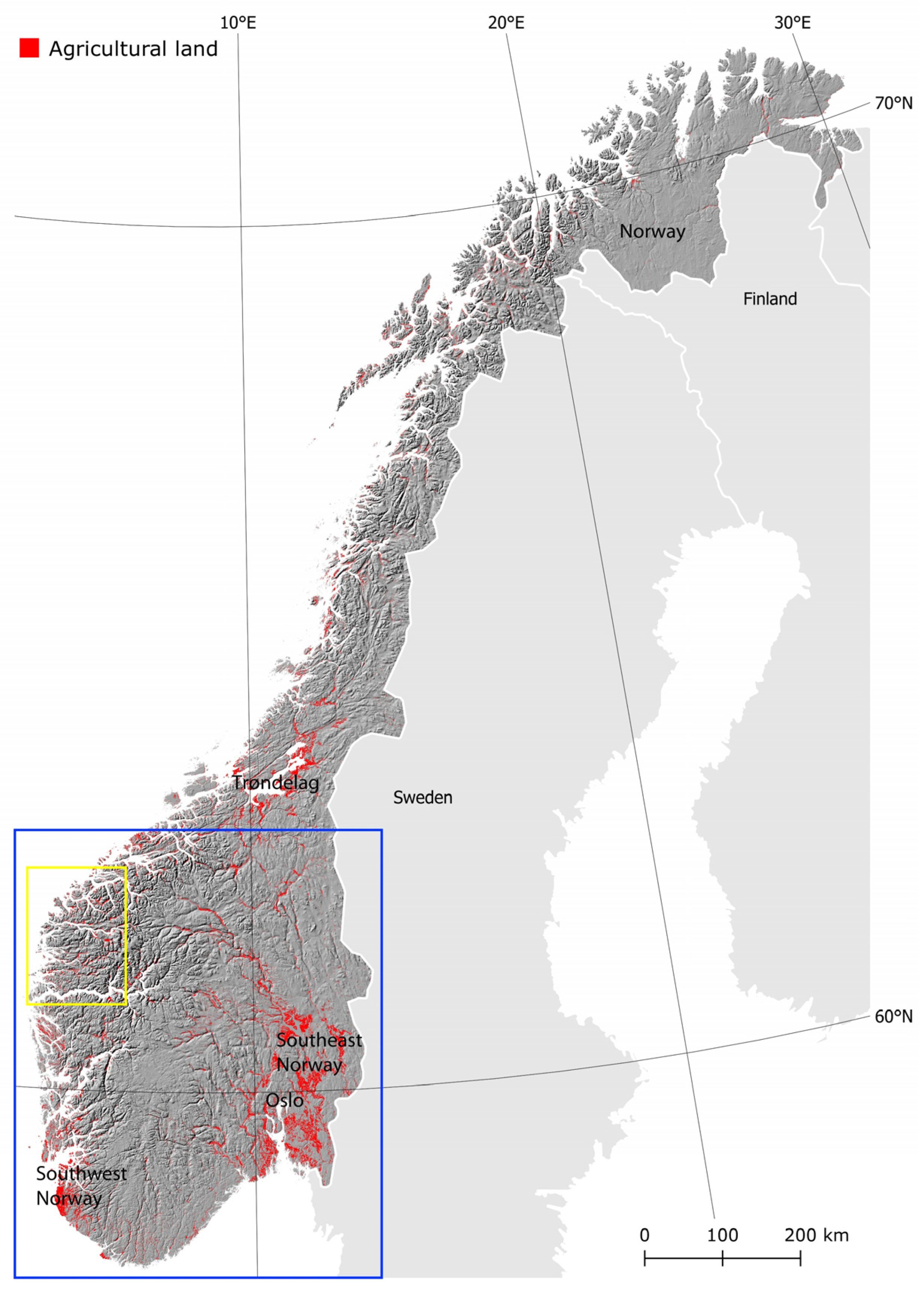
The study area comprises mainland Norway and islands along the coast, covering 324,000 km² from 58° N to 71° N and from 5° E to 31° E. Norway is positioned along the north-west Atlantic coast and forms a part of the Scandes mountain chain (Figure 2). The topography goes from sea level up to 2469 m above sea level, with around 40% of the area above the treeline. The landforms vary from gently undulating paleic landscapes of southeast and northeast Norway to steep fiords and alpine landscapes in all western parts of the country.

Importantly for agriculture, many lowland regions have marine clay deposits that today host the main bulk of the grain production in three regions of Norway: southeast Norway, southwest Norway and Troendelag. Throughout the rest of Norway, agriculture appears along valley and fjord bottoms, or scattered around on locations with good soils and acceptable climate [54]. Presently, agricultural farmland covers 3% of the land area in Norway, but much more of the land is utilized for domestic and semi-domestic grazing [55] in the outfields (areas outside the agricultural land, for example heaths and forests). Compared with other EU countries, the agriculture of Norway is small-scaled and extensive, with 2/3 of the farmers producing milk or meat. The most common agricultural land use is therefore livestock grazing and grass production. The number of active farmers (that claimed subsidy) in 2019 was 39,090, whereas the number of farms in 1969 was 154,977 [56]. However, in this context it is worth noting that the total farmed area in Norway has not been much affected by the exodus of farmers from the industry [56].

2.2. The Norwegian Subsidy System

The agricultural subsidy system in Norway is rather complex, and the current agricultural policy regulates subsidies towards several factors, such as type of production, farm sizes and regional affiliation. However, most subsidies are based on coupled payments with rates which are negatively related to farm size [57]. In regions with disadvantageous climate, such as far north or at high elevations, the payment rates are higher. Payments rates are also higher for organic farming, and outfield domestic grazing is supported by specific programs. High border protection against food imports drives domestic market prices well above world market levels [58]. Still, subsidies in Norway make up the largest part of farmers’ income, considerably exceeding market-based gross margins in most farming activities. It is therefore important for the farmers’ income to actively claim subsidies for all land use parcels.

2.3. Data Preparation—Land Parcel ID Data

The subsidy claim is made under the farm code of the farmer’s “home farm” (we use the term for convenience, there may in fact be no resident farmer), and the codes of any land claimed for (whether owned or rented) are included in each claim. The Norwegian Agricultural Authority (NAA) database containing these subsidy claims is hereafter referred to as the production subsidy data and land parcels IDs as LPIDs (LPID refer to the stable identity number of the land parcel within the database).

The implemented dataset consisted of fourteen years of subsidy claim records (2003–2016) for approximately 60,000 farms claiming for around 200,000 land parcels. The LPIDs are part of the Norwegian cadastral system and are thus geo-referenced to a polygon map layer.

Individual land parcels may be sold or rented between farm businesses over the period, yet there is no relational database structure linking LPIDs, thus no simple database query could establish which years a particular LPID was in use/out of use. A script was implemented in Visual Basic for Applications (VBA) for MS Access to sift the database for each LPID and then assign a “1” or “0” to a given year depending, respectively, on whether a match was found. The result was a binary string for the presence and absence of each LPID over the time period (

Table 1. Example illustrating the database structure having assigned each land parcel a unique ID (Parcel ID Number; all IDs have been changed for privacy reasons), a zero value (not claimed for) or a value of one (claimed for) for each of the years 2003 to 2016.

Parcel ID Number	a2003	a2004	a2005	a2006	a2007	a2008	a2009	aQ 2010	aQ 2011	aQ 2012	a 2013 E	a 2014 E	a 2015 E	a 2016 E
XXXX	1	1	1	1	1	0	0	0	0	0	0	0	0	0
XXXX	1	1	1	1	1	1	1	1	1	1	1	1	1	1
XXXX	0	0	0	0	0	1	1	1	1	1	1	1	1	1
XXXX	1	1	1	1	1	1	1	1	1	1	1	1	1	1
XXXX	0	0	0	0	0	0	0	0	0	0	0	0	0	0
XXXX	1	1	1	1	1	1	1	1	1	1	1	1	1	1
XXXX	1	1	1	1	1	1	1	1	1	1	1	1	1	1
XXXX	0	0	0	0	0	0	0	0	0	0	0	0	0	0
XXXX	0	0	0	0	0	0	0	0	0	0	0	0	0	0

).

2.4. Analyses—Descriptive Abandonment Statistics

The binary string was used to generate five types of descriptive statistics for each LPID (

Table 2. The five classes of descriptive statistics and methodology explained.

Type of Classification	Method
Average	The simple average between 0 and 1 for all years
Three Year Shocks	The number of periods of three years or more where no claim was made, followed by a recorded return to production or the end of the study period
Balance	The sum of the last seven years, minus the sum of the first seven years
Logistic Regression Line	Trend in likelihood of use as a logistic regression line fitted through the time series
Long-Term Outlook	The logistic regression line classification, with all those points for which a line could not be fitted classified to either 1 or 0 based on their majority state

). The five approaches reveal different aspects of the usage pattern of the land parcel.

Average: The calculated average gives a general impression of the overall land use during the period. However, a two-year rotational fallow will give a similar value as regular use for the first seven years followed by complete abandonment for the following seven. The statistic is slightly sensitive to start and end dates, and ignores trends.

Three Year Shocks: The absence of any usage for three or more years probably provides a sufficiently long period to initiate some habitat and land quality changes. While the extent and severity will differ, e.g., by location, it is likely there will be increased investment required to restore the land to a fully cultivated status. It therefore suggests something has occurred for that land parcel such as change of ownership or unfavorable economic or weather conditions. Therefore, while this index indicates that something is not optimal for a land parcel, it could be that the “shock” is far longer (up to ten years) or followed by ten years of use. There is no way to reliably distinguish this from absence in the last three years of the time series, for example. This index is likely to be more useful with longer time series.

Balance: A large differential between the former and latter halves of the 14-year time period would suggest at the least a significant longer-term downgrading of that land parcel’s productivity compared with its potential as evidenced by the first half usage. This index seems reasonable at least where there is big change; however, it is also slightly sensitive to start and end dates.

Logistic Regression: The concept of fitting a regression line through a time series of 0 and 1 values may appear counterintuitive at first sight. However, the regression line is not fitted to the binary values, per se, rather it is fitted to the probability that a prediction of either 1 or 0 is correct for any given year.

Table 3. An example illustrating the use of a time series of binary variables as basis for a regression. See text for further explanation.

Parcel ID Number	a2003	a2004	a2005	…	a 2014 E	a 2015 E	a 2016 E	X1 Intercept	Coeff X1
XXXX	1	1	1	…	0	0	0	18.56606861	−19.66468079
XXXX	1	1	1	…	1	1	1	25.56606935	−9.93607391
XXXX	0	0	0	…	1	1	1	−18.56606851	−19.66468079
XXXX	1	1	1	…	1	1	1	25.56606935	−9.936073912
XXXX	0	0	0	…	0	0	0	−25.56606852	−4.144585628
XXXX	1	1	1	…	1	1	1	25.56606935	−9.936073912
XXXX	1	1	1	…	1	1	1	25.56606935	−9.936073912
XXXX	0	0	0	…	0	0	0	−25.56606852	−4.144585628
XXXX	0	0	0	…	0	0	0	−25.56606852	−4.144585628

highlights one example. If one were to predict a “1” for each year of the first five years in the first row with data (Table 3), the result would be 100% correct, but for the first six years it would only be correct 83.4% of the time, for the first nine years it would be correct only 55.6% of the time, and by year eleven only 45.5% of the time. Therefore, there is a trend in the probability that a prediction of “1” (or “in use”) would be correct for any given year as time goes on. The rate of change in that probability is given by the coefficient (−19.66 in this case indicating a declining probability of use). Logistic regression can thus help to inform the concept of Munroe et al. [21] of abandonment in terms of a longer term trajectory, and can provide error limits on that trajectory. In theory, the demonstrated trend may also be correlated with other possible drivers of that process, however the data period used here is too short to allow this to be analyzed. In order to fit a trend, the dataset needs to provide a sufficient number of examples to see a clear trend in probability, thus the stronger the trend the fewer examples are required, but a rule of thumb would suggest a minimum of ten data points per variable. Therefore, to establish explanatory correlations with a view to predicting future change this suggests 20 years would be necessary. Of course, that ‘rule’ is only a general target figure, it is also impacted by the strength of the trend found.

Long-Term Outlook: Logistic regression only functions when the probability is not too extreme. As the probability approaches 0 or 1, the function fails. However, in those circumstances the outlook of the land parcel is clear: either it is in regular use and showing little evidence of that changing, or it is rarely if ever used. Thus, a composite index may be developed showing the likely outlook for all the land parcels by assuming the values of 1 and 0, respectively, for these cases and providing the logistic trend line for cases in between.

3. Results

3.1. Abandonment Metrics

The following five maps show the abandonment metrics described. The results are averaged by 5 km and 10 km grid squares to prevent the identification of the data for the land of any individual farmer. The 5 km and 10 km grid squares are used because these are standard units from Statistics Norway which are used in surveys to collect a range of relevant land use and land cover information. It should be remembered that the total number of LPID may vary considerably, and the Modifiable Area Unit Problem (MAUP) may influence the pattern [59]. For example, an alternative to anonymizing the data would be one or more interpolation methods, each of which might produce slightly different results by aggregating and smoothing the data differently.

3.2. Average

Figure 3 shows the results of the Average index, i.e., the mean number of years in use for each land parcel. In this map, land use parcels (LUP) that have no use during the period are also included in our analyses, i.e., what may be described as historical loss. We know from agricultural statistics that a large number of smaller and less accessible or less easily manageable parcels have been taken out of use over a long period of time prior to the period included in our geographical analyses. A metric such as the mean number of years in use will accumulate this, and this will have an effect on the results. The metric still illustrates where there is less or more continuous use of agricultural land use parcels.

In interpreting the map (Figure 3), it is important to remember that the result includes land use parcels that may have no use during the analyzed period. As can be seen from the map, the cells with lower use appear to occur in a rather dispersed manner. There are parcels scoring a value toward 1 (i.e., used all years) and parcels scoring a value at or close to 0 (i.e., only used one or a few years). There are some general areas of lighter or darker color, but when zooming into the 5 km aggregation on the right map, much diversity within these areas become apparent. It is also important to keep in mind that this index does not distinguish between use at the beginning or end of a period nor cyclical changes. This can be important, as we know from statistics in Norwegian agriculture that the number of active farmers continues to decline, and this can be expected to be discernible also as a trend in parcel use. Yet, the mean statistics over time could show similar values for these three very different cases. To include this in the evaluation, we decided to also calculate what we have called “Balance” (Figure 4).

3.3. Balance

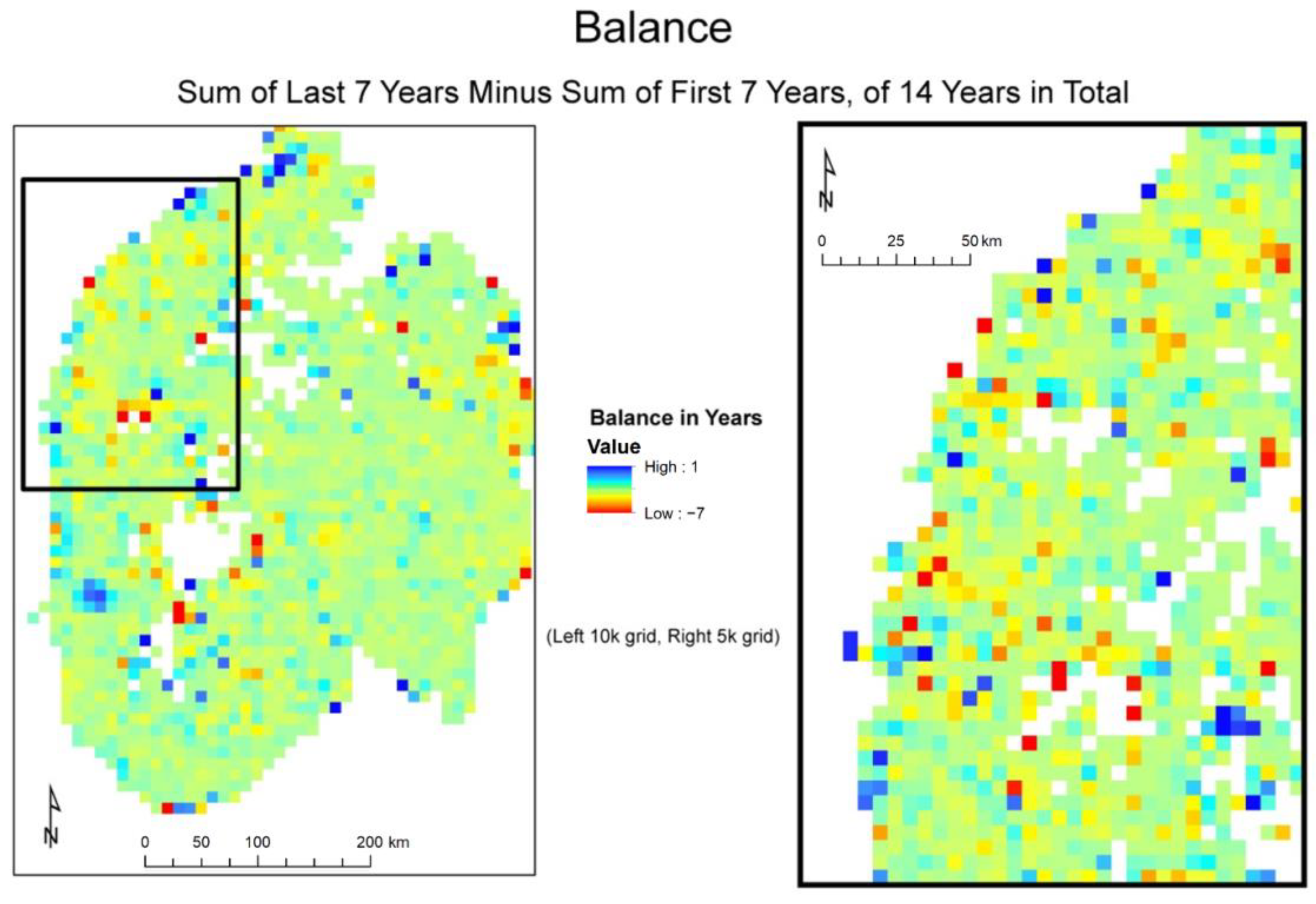
This index is calculated by subtracting the sum of years in use during the first seven years from the sum of years in use during the last seven years. This way, time is integrated in the index and map in a way that enables the differentiation as to what direction of change there may have been. A positive result thus implies more use of land parcels during the more recent period. A negative result would indicate a declining use. The resulting map is displayed in Figure 4.

Reviewing the output, it is apparent that the middle of the range is highly sensitive to the boundary effect of the time period (i.e., one year either way might tip it from positive to negative). For this reason, the map is four-colored, with the central range being green either side of zero; this distinction is arguably of little value. A tri-color option was considered but seemed equally open to “intuitive” erroneous reading. Therefore, the metric seems somewhat risky for visualization. It does, however, highlight strong changes. While there are some patches of blue (indicating increased usage) at the 10 km grid, these could be random effects of classification unit since zooming to 5 km reveals more coherent areas of orange/red, indicating quite large declines in use between the two halves of the period. The smaller spatial scale of aggregation reveals higher variance particularly in the yellow to red range, this suggests a skew toward more cases of decline. However, range and scale sensitivity should also decline with longer time scales as individual parcel years become proportionately smaller.

3.4. Three Year Shocks

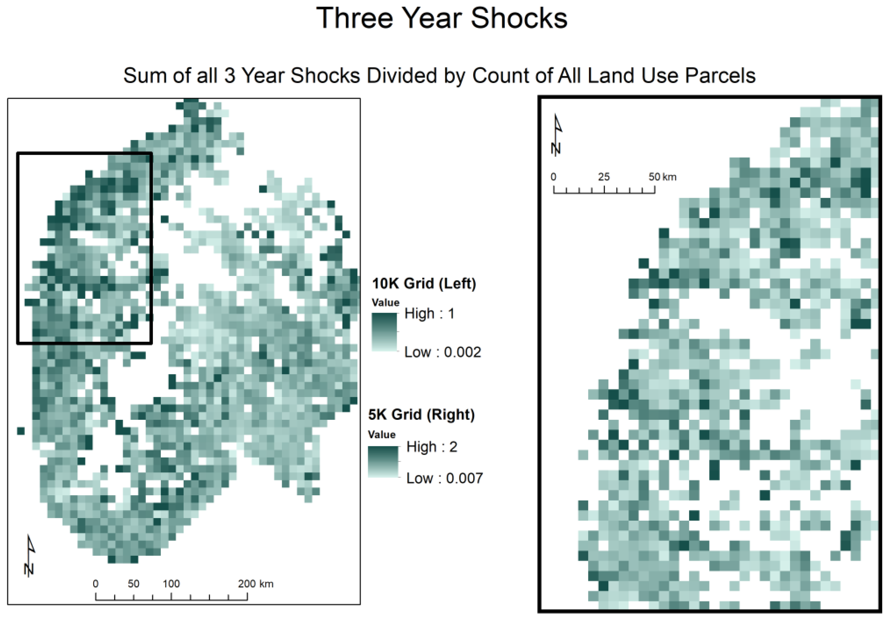
While the “balance” will differentiate between former and more recent time periods, it does not differentiate well in terms of the practice of leaving land fallow for certain periods. Leaving land fallow could be part of an agricultural practice, or occur due to random events (illness, generation shifts, selling land, high parasitic pressure in pastures, etc.). We anticipate that such events will normally last for one, and on rare occasions, two years. If land is out of use for three years, it will both be apparent that vegetation is changing, and the land will probably display a change in visual and agronomic functions. We thus decided to calculate whether any periods of three years with no apparent use could be identified (Figure 5).

This map shows the total count of three-year shocks in a given cell (i.e., regardless of whether it may be several shocks to the same LUP or a single shock to several LUP). That figure is then normalized by the total number of claiming LUP in the cell (i.e., excluding historical losses but including those LUP with no claims at all in this time period). It is also worth noting that the 10 km grid shows a value range from zero to 1, while the 5 km ranges up to 2. This is due to statistical averaging. In fact, the highest number of shocks recorded for any one parcel was 3 in the 14-year period, but this is so rare that no cells show this value on average (the full range would appear in the point map of the parcels, but this cannot be published for privacy reasons).

There is a clear gradient from west to east with proportionately more shocks to the west and certain valleys running inland from the west coast seem to have higher numbers of shocks. To know whether this represents a low-grade issue affecting many LUP in a cell, or a more intense problem repeatedly affecting a subset of the LUP, the map could be redrawn to highlight mean shock rate per LUP per cell rather than mean number of shocks per LUP per cell.

3.5. Logistic Regression

This analysis emphasizes even more the temporal aspect. The result (Figure 6) is a trend in the probability that a prediction of “1” (that is “in use”) would be correct for any given year as time goes on (red shades indicate declining probability of “in use”, whereas blue shades indicate increasing probability of “in use”). The rate of change in that probability is given by the coefficient of a binary logistic regression. Regression coefficients were only achieved for 92,322 LUP (or just under half the data set) and only these are considered here. The reason only half of the LUP can be characterized in this way is principally due the fact that the rest are basically stable LUP (either entirely out of use or entirely in use), but also that 14 data points is relatively few for the method; as more years become available, more LUPs can be included.

The map displays the slope of the trend in probability of use. Shades of green color suggests a basically stable situation, with very little trend either way. This does not mean the LUP is necessarily being frequently used, only that the trend is flat. For example, if an LUP is used only twice, both at the start of the period, this would lead to a strongly negative trend, but if it was used once in year 1 and once in year 14, it would be a flat trend. To distinguish between a flat trend which represents high use and flat trend representing low use, the intercept can be used. This has one remaining limitation, however. If a trend could not be calculated for the LUP then no intercept is available. Therefore, it is alternatively proposed to combine this measure with a more blunt metric, the sum of years in use, in order to create a composite measure, the Long-Term Outlook.

3.6. Long-Term Outlook

To put the stable LUPs back into the picture, the cells with very high or very low average use were overlain on the regression coefficient map (Figure 7). The Long-Term Outlook metric supplements the logistic regression with a simple mask overlay distinguishing between flat trends due to infrequent or no use, and flat trends due to frequent or constant use. Other values in the mask layer are transparent, thus continuing to display the positive or negative trends in between these two extremes. In doing so, it overrides the logistic regression result where those LUPs with a trend are such a small minority that the overall picture is either basically in use or basically abandoned. At the same time, the user can set the limit for the total numbers of years in use/out of use to consider as productive/abandoned and the mean to be reached before this binary mask is overlaid. In this way the metric can be adjusted to highlight only the most extreme trends or all trends, and to model those where this is the majority case. Each way of viewing the metric applies to different landscape management goals such as viewing present change (no mask) or viewing landscapes at risk (masking only those areas with a majority of LUPs in very low use.)

Reviewing the map (Figure 7), it is apparent that most of the areas showing a dispersed clustering of negative average coefficient are also areas with high levels of historical loss (Figure 4). The areas of highest average use from Figure 3 (e.g., patches southeast of Oslo and along the coast) show a generally neutral to positive picture (shades of green in Figure 7) unless the cell has already seen high historical loss. It is an interesting question as to why any cell might see a positive Long-Term Outlook, i.e., the land is not used every year but is being used more frequently. If such a trend can be established for a whole 10 km cell this would be an interesting exception to the national picture. However, it more likely serves to accentuate the point that land use is dynamic and thus the period of study is critical.

The two entirely positive blue patches are a statistical flaw due to introduction of new data and changing borders of municipalities during the time period analyzed: changing the municipality numbers makes the parcel appear newly in use. Municipality changes elsewhere have been controlled for by “back casting” the new codes, but in this locality that was not possible due to lack of the necessary information as to what changes occurred when. A limitation to adopting the method is therefore whether a country can establish reliable time series. However, although Norway has particularly good records, the principle that temporal patterns of change can be measured by multiple metrics is useful more generally.

4. Discussion

Our work indicates that abandonment is not a binary process. We rarely observed a simple trajectory from “in use” to “out of use” for any particular land use parcel. The real agricultural world is much more dynamic, at least for Norway. The dynamism is likely the result of a wide range of more or less continuously ongoing processes, such as changes in subsidy regimes, generation transitions, investments, fallowing, technological development, etc. These processes are documented in general [7,8,17,22,43,44,45], but their effect on the actual use of land is more uncertain. Assessing the continuity of use for each agricultural land use parcel independently, the main message from our results is a much higher turnover of LUPs than expected.

Regarding abandonment of agricultural land parcels, it should not come as a surprise that land parcels go in and out of use. It is well known how, in times of crises, food is produced wherever possible (Figure 1). In scientific studies, outside those involving remote sensing-based time-series, it seems that time-series is less frequently considered, however, and we would like to argue that this should become more common. In Norway, there is a clear trend that land that has been used for agriculture is abandoned. However, there is also land that is brought back into production. These two factors combined point to an increasingly fragmented agricultural landscape in future which could lower production (e.g., because of larger edge-effects), but with large geographical variation.

The different metrics highlight different patterns. However, there are some consistencies, for example, the west coast, highlighted in the right hand zoom box for each example, seems to show consistent cause for concern with respect to food production, as do certain valleys therein. This is perhaps the principal advantage of using several metrics; while all metrics will be affected by the time window of the study, they are all affected in different ways. Therefore, if a consistent picture is seen across several metrics, then more confidence can be attributed to this impression than for a single metric.

The metrics all indicate high spatial variation, but also provide a clear spatial picture, i.e., geography matters. When we included all land parcels that had been recorded as in agricultural use, the results demonstrated a significant and widespread decline. This was clearly apparent when we calculated average years every land parcel had been used during the studied period (Figure 3).

The length of the period land parcels remained out of use varied. This led us to the conclusion that we had to use a time limit in our definition of abandonment, and we decided that it was not until a field had remained unused for three years that we would describe it as abandoned. This was based on a reasoning where one year could be an arbitrary event (e.g., machine breakdown or illness or even deliberate fallow), two years could still be e.g., through a process of selling a farm or renting out land, but after three years vegetation would also begin to change in terms of onset of a natural succession, thus falling within the definitions e.g., by Eurostat [26] or Keenleyside and Tucker [12]. However, simply using this three-year extent as a decisive factor in the analyses did not give us as much information as we believe the data held. We wanted to be able to demonstrate trends over time, and thus a three-year long abandonment in the beginning of our 14-year study period would represent a different trend from a three-year abandonment period towards the end of our study period. To add this information, we decided to divide our period in two and look for the “balance”.

Still, we wanted to assess whether the trend over time was in fact positive, defined as more land being brought back into production or negative, defined as more land being abandoned over time. To analyze this, we found that logistic regression was an interesting method as this would give the trend in usage frequency. In that respect it is the most complete and robust of the metrics. It is, however, sensitive to the position of the absence (out of use) or presence (in use) during the time period (either end is weightier), and as such could be sensitive to a one-year difference in time period. The degree of sensitivity is dependent on time series length and the strength of the trends to be found. Consequently, in the case of univariate regression over a relatively short time period as here, the error statistics must be considered to be affected by the precise period chosen also, which introduces some uncertainty beyond what they can capture from the data within that window. For this reason, predicting when a parcel might reach some threshold of abandonment should be used cautiously, but the error statistics still help to indicate the confidence with which the trend is established.

However, as data accrues with each passing year the technique can become more precise, GLM also outputs various other values. In principle these could be used to predict when the probability of usage will drop below, e.g., 30% and thus the land might be considered abandoned. In this case, however, (a) we do not have enough years to reliably extrapolate, we can only see the previous frequency not the future probability and (b) we do not have enough years to compare with potential drivers. As with the univariate case the same caveat applies with respect to using error statistics to predict how trends in the explanatory variables might be used to identify when in the future a threshold of abandonment is reached, particularly given that the rule thumb regards 10 data points per variable. However, mapping the residuals could at least provide some confidence as to where the explanatory variables were consistently effective and where not.

There are limitations and several sources of potential error in these analyses, and also differing sources of uncertainties. For example, local variation in abandonment is averaged over 5 km and 10 km, restricting map users’ access to farm-specific information. Regarding the analyses of the regression coefficient, it is important to be aware that even a slightly different time period might “tip” the trend. Additionally, although the overall picture remains slightly positive, there are regional variations in the number of 5 km squares with substantially negative trends. Because these are generally dispersed, individual values will be subject to spatial unit variation. It is likely a similar dispersion pattern would pertain to a different grid origin, and that larger grid square would see aggregation effects. Were the intent to analyze the maps in grid form, one might then also consider more sophisticated interpolation methods to optimize spatial precision where data density allows this without aggregating an individual’s data. However, this method is intended to be used at parcel level by Norwegian authorities with full data access. The purpose here is only to illustrate aspects of the results from the different measures, not suggest their presentation at any particular scale. The appropriate aggregation or anonymization method when deployed elsewhere would therefore be dependent on the national context and audience.

Still, we do have a method that, with accumulation of years, could be used to analyze the drivers of frequency of use. For example, with reliable error margins on the coefficient, these could be subjected to a Monte Carlo process, and the results regressed spatially against production data or ownership/rental type. In addition, when reading the regression map it is important to bear in mind that all the “no change” is absent. Since most changes are negative, that easily gives an impression of more negatives than in reality. Equally there could be areas of consistent lack of use. Therefore, a regression map must always be accompanied by a map of “always in use” and another of “never in use” which we have combined into one map, the Long-Term Outlook.

Also important is the effect that using a sloping dummy variable has, particularly on the negative coefficients; they look a little more negative (or less positive) than they actually are. A full presence should really provide a value of zero (flat line) but the effect of rounding in a finite computer would result in a small positive or negative at random of some small but indeterminate size. We would then be unable to separate this from, e.g., a real but tiny decline in usage (e.g., −9 × 10⁻⁸) or a full absence (all zero) which should also give zero but now gives −1 × 10⁻¹⁶ Of course, all zero and all one can be identified by query, but it is useful to be able to distinguish the cases and more importantly to not assume one can classify by zero precisely. With more years accrued, the precision increases, which reduces the issue.

Alongside methodological limitations and uncertainties, the data is accompanied with potential errors. By method, the presumption in this study is that there is a direct link between actual use of a parcel and the subsidy claim. However, there is no way to know whether a parcel in fact was in use the year a farmer applied subsidies for it. Additionally, vice versa, there is no way to know if a parcel in fact was in use, but without subsidies being applied for. The effects of such errors will depend on the reliability of the subsidy database. The advantage of the tested database is the importance of subsidy claims for the farmers’ income, combined with a systematic control regime. Another solution could be to test the reliability of a sub-set of the database by use of for example satellite remote sensing or high-resolution aerial photos [8,10].

Perhaps the strongest lesson from these metrics is that a single metric does not suffice. Agriculture is a complex business with many different forms, practices and products. Some will have longer term cycles than others. In addition, there are a large number of decision-makers sensitive to a wide range of drivers. Only by “triangulating” different metrics that emphasize different aspects of change over time, and by looking at spatial patterns across scales, can one begin to build up a picture of what trends represent broader and deeper implications for the landscape. We believe this could potentially provide highly useful information to management and policymakers.

5. Conclusions

The assessment of subsidy data targeted at specific land unit parcels, convinced us that a binary view on agricultural abandonment is restricting any analyses aiming for a deeper understanding of abandonment. We propose that the often static term “abandonment” be reconsidered to better encompass temporal dynamics. The data from Norway show that LUPs are frequently shifting back and forth between “abandoned” and operative, although some LUPs also are lost. Land parcels are removed from agricultural production but also added again, and there appears to be considerably higher dynamics in land management than previously accounted for. It is thus clear that when discussing abandonment, a temporal component could preferably be included.

In mapping and measuring abandonment of agricultural land in Norway, we developed and tested five metrics. Our analyses demonstrated how various measures capture different aspects of frequency of use of agricultural land. The best procedures to use in any given case will be context dependent. The advantage of using several metrics is that if a consistent development of frequency of use is supported, then more confidence can be attributed to the interpretation. It is, however, clear from our results that abandonment shows some spatial patterns, suggesting that regional context may be important.

If we are to meet the global aims of producing more food while reversing the loss of biodiversity, halting climate change and ensuring fulfilment of the sustainable development goals, we need to optimize our land use. In this process, abandoned agricultural land may have important roles to play. However, to be able to activate this possibility, we need to be able to map and measure it. The metrics developed, tested and reported in this paper may represent a first step in this process.

References

1. Intergovernmental Panel on Climate Change—IPCC. Climate Change and Land. An IPCC Special Report on Climate Change, Desertification, Land Degradation, Sustainable Land Management, Food Security, and Greenhouse Gas Fluxes in Terrestrial Ecosystems; Summary for Policymakers; WHO: Genève, Switzerland; UNEP: Nairobi, Kenya, 2019. [Google Scholar]
2. Albrecht, J.; Carrez, D.; Cunningham, P.; Daroda, L.; Mancia, R.; Mathé, L.; Achim Raschka, A.; Carus, M.; Piotrowski, S. The Knowledge Based Bio-Economy (KBBE) in Europe: Achievements and Challenges; Clever Consult Technical Report; Clever Consult BVBA: Meise, Belgium, 2010. [Google Scholar]
3. Anand, M. Innovation and Sustainable Development: A Bioeconomic Perspective; Brief for Global Sustainable Development Report 2016; United Nations Division for Sustainable Development Goals: New York, NY, USA, 2016. [Google Scholar]
4. Heimann, T. Bioeconomy and SDGs: Does the bioeconomy support the achievement of the SDGs? Earth’s Future 2019, 7, 43–57. [Google Scholar] [CrossRef] [Green Version]
5. Foley, J.A.; Ramankutty, N.; Brauman, K.A.; Cassidy, E.S.; Gerber, J.S.; Johnston, M.; Mueller, N.D.; O’Connell, C.; Ray, D.K.; West, P.C.; et al. Solutions for a cultivated planet. Nature 2011, 478, 337–342. [Google Scholar] [CrossRef] [PubMed] [Green Version]
6. Benayas, J.R.; Martins, A.; Nicolau, J.M.; Schulz, J.J. Abandonment of agricultural land: An overview of drivers and consequences. CAB Rev. 2007, 2, 1–14. [Google Scholar] [CrossRef] [Green Version]
7. Meyfroidt, P.; Chowdhury, R.R.; de Bremond, A.; Ellis, E.C.; Erb, K.-H.; Filatova, T.; Garrett, R.D.; Grove, J.M.; Heinimann, A.; Kuemmerle, T.; et al. Middle-range theories of land system change. Glob. Environ. Chang. 2018, 53, 52–67. [Google Scholar] [CrossRef]
8. Yin, H.; Brandao, A.; Buchner, J.; Helmers, D.; Iuliano, B.G.; Kimambo, N.E.; Lewinska, K.E.; Razenkova, E.; Rizayeva, A.; Rogova, N.; et al. Monitoring cropland abandonment with Landsat time series. Remote Sens. Environ. 2020, 246, 111873. [Google Scholar] [CrossRef]
9. Anderson, E.; Mammides, C. Changes in land-cover within high nature value farmlands inside and outside Natura 2000 sites in Europa: A preliminary assessment. AMBIO 2020, 49, 1958–1971. [Google Scholar] [CrossRef]
10. Aune, S.; Bryn, A.; Hovstad, K.A. Loss of semi-natural grassland in a boreal landscape: Impacts of agricultural intensification and abandonment. J. Land Use Sci. 2018, 13, 375–390. [Google Scholar] [CrossRef]
11. Fuchs, R.; Verburg, P.H.; Clevers, J.G.P.W.; Herold, M. The potential of old maps and encyclopaedias for reconstructing historic European land cover/use change. Appl. Geogr. 2015, 59, 43–55. [Google Scholar] [CrossRef] [Green Version]
12. Keenleyside, C.; Tucker, G.M. Farmland Abandonment in the EU: An Assessment of Trends and Prospects; Report for WWF Netherlands; Institute for European Environmental Policy: London, UK, 2010. [Google Scholar]
13. Pointereau, P.; Coulon, F.; Girard, P.; Lambotte, M.; Stuczynski, T.; Sánchez Ortega, V.; Del Rio, A. Analysis of Farmland Abandonment and the Extent and Location of Agricultural Areas That Are Actually Abandoned or Are in Risk to be Abandoned; JRC Scientific and Technical Reports EUR 23411EN; Joint Research Centre: Ispra, Italy, 2008. [Google Scholar]
14. Food and Agriculture Organization—FAO. The Role of Agriculture and Rural Development in Revitalizing Abandoned/Depopulated Areas; Food and Agriculture Organization of the United Nations: Rome, Italy, 2006. [Google Scholar]
15. Hart, J.F. Loss and abandonment of cleared farm land in the eastern United States. Ann. Assoc. Am. Geogr. 1968, 58, 417–440. [Google Scholar] [CrossRef]
16. Kuntz, K.; Beaudry, F.; Porter, K. Farmers’ perceptions of agricultural land abandonment in rural western New York State. Land 2018, 7, 128. [Google Scholar] [CrossRef] [Green Version]
17. Osawa, T.; Kohyama, K.; Mitsuhashi, H. Multiple factors drive regional agricultural abandonment. Sci. Total Environ. 2016, 542, 478–483. [Google Scholar] [CrossRef] [PubMed]
18. Yu, Z.; Lu, C. Historical cropland expansion and abandonment in the continental U.S. during 1850 to 2016. Glob. Ecol. Biogeogr. 2008, 27, 322–333. [Google Scholar] [CrossRef]
19. Ceaușu, S.; Carver, S.; Verburg, P.H.; Kuechly, H.U.; Hölker, F.; Brotons, L.; Pereira, H.M. European Wilderness in a Time of Farmland Abandonment. In Rewilding European Landscapes; Pereira, H.M., Navarro, L.M., Eds.; Springer: Berlin/Heidelberg, Germany, 2015; pp. 25–46. [Google Scholar]
20. Haddaway, N.R.; Styles, D.; Pullin, A.S. Environmental impacts of farm land abandonment in high altitude/mountain regions: A systematic map of the evidence. Environ. Evid. 2013, 2, 18. [Google Scholar] [CrossRef] [Green Version]
21. Munroe, D.K.; van Berkel, D.B.; Verburg, P.H.; Olson, J.L. Alternative trajectories of land abandonment: Causes, consequences and research challenges. Curr. Opin. Environ. Sustain. 2013, 5, 471–476. [Google Scholar] [CrossRef]
22. Terres, J.M.; Scacchiafichi, L.N.; Wania, A.; Ambar, M.; Anguiano, E.; Buckwell, A.; Coppola, A.; Gocht, A.; Källström, H.N.; Pointereau, P.; et al. Farmland abandonment in Europe: Identification of drivers and indicators, and development of a composite indicator of risk. Land Use Policy 2015, 49, 20–34. [Google Scholar] [CrossRef]
23. Van der Zanden, E.H.; Verburg, P.H.; Schulp, C.J.E.; Verkerk, P.J. Trade-offs of European agricultural abandonment. Land Use Policy 2017, 62, 290–301. [Google Scholar] [CrossRef]
24. Poore, J.A.C. Call for conservation: Abandoned pasture. Science 2016, 351, 132. [Google Scholar] [CrossRef] [PubMed]
25. Asheim, L.J.; Thorvaldsen, P.; Rivedal, S. Policy measures to preserve Norwegian coastal and fjord landscapes in small-scale farming systems. Environ. Sci. Policy 2020, 104, 43–51. [Google Scholar] [CrossRef]
26. Eurostat. Agri-Environmental Indicator—Risk of Land Abandonment; Statistics Explained; Eurostat: Luxembourg, 2013.
27. Beilin, R.; Lindborg, R.; Stenseke, M.; Pereira, H.M.; Llausas, A.; Slatmo, E.; Cerqueira, Y.; Navarro, L.; Rodrigues, P.; Reichelt, N.; et al. Analysing how drivers of agricultural land abandonment affect biodiversity and cultural landscapes using case studies from Scandinavia, Iberia and Oceania. Land Use Policy 2014, 36, 60–72. [Google Scholar] [CrossRef]
28. Bignal, E.; McCracken, D. The nature conservation value of European traditional farming systems. Environ. Rev. 2000, 8, 149–171. [Google Scholar] [CrossRef]
29. Dover, J.W.; Rescia, A.; Fungarino, S.; Fairburn, J.; Carey, P.; Lunt, P.; Arnot, C.; Dennis, R.L.H.; Dover, C.J. Land-use, environment, and their impact on butterfly populations in a mountainous pastoral landscape: Species richness and family-level abundance. J. Insect Conserv. 2011, 15, 523–538. [Google Scholar] [CrossRef]
30. Hunziker, M. The spontaneous reafforestation in abandoned agricultural lands—Perceptions and aesthetic assessment by locals and tourists. Landsc. Urban Plan. 1995, 31, 399–410. [Google Scholar] [CrossRef]
31. García-Ruiz, J.; Lana-Renault, N. Hydrological and erosive consequences of farmland abandonment in Europe, with special reference to the Mediterranean region—A review. Agric. Ecosyst. Environ. 2011, 140, 317–338. [Google Scholar] [CrossRef]
32. Flury, C.; Gotsch, N.; Rieder, P. Site-specific and regionally optimal direct payments for mountain agriculture. Land Use Policy 2005, 22, 207–214. [Google Scholar] [CrossRef]
33. Food and Agriculture Organization—FAO. The Future of Food and Agriculture: Trends and Challenges; Food and Agriculture Organization of the United Nations: Rome, Italy, 2017. [Google Scholar]
34. Porter, J.R.; Xie, L.; Challinor, A.J.; Cochrane, K.; Howden, S.M.; Iqbal, M.M.; Lobell, D.B.; Travasso, M.I. Food Security and Food Production Systems. In Climate Change 2014: Impacts, Adaptation, and Vulnerability. Part A: Global and Sectoral Aspects; Contribution of Working Group II to the Fifth Assessment Report of the Intergovernmental Panel on Climate Change; Field, C.B., Barros, V.R., Dokken, D.J., Mach, K.J., Mastrandrea, M.D., Bilir, T.E., Chatterjee, M., Ebi, K.L., Estrada, Y.O., Genova, R.C., et al., Eds.; Cambridge University Press: New York, NY, USA, 2014; pp. 485–533. [Google Scholar]
35. Kent, C.; Pope, E.; Thompson, V.; Lewis, K.; Scaife, A.A.; Dunstone, N. Using climate model simulations to assess the current climate risk to maize production. Environ. Res. Lett. 2017, 12, 054012. [Google Scholar] [CrossRef]
36. Lågbu, R.; Nygård, Å.; Svendgård-Stokke, S. Jordsmonnstatistikk i Norge; NIBIO Rapport 4; Norwegian Institute for Bioeconomy Research: Ås, Norway, 2018. [Google Scholar]
37. Montanarella, L.; Pennock, D.; McKenzie, N. Status of the World’s Soil Resources; Technical Summary; Food and Agriculture Organization of the United Nations: Rome, Italy, 2015. [Google Scholar]
38. Elde, S.; Kvalvik, I.; Nøstvold, B.H.; Rødbotten, R.; Dalmannsdottir, S.; Halland, H.; Uleberg, E.; Reykdal, Ó.; Árnason, J.; Pálsson, P.G.; et al. The Arctic as a Food Producing Region. Phase 1: Current Status in Five Arctic Countries; NOFIMA Report 10-2018; Nofima AS: Tromsø, Norway, 2018. [Google Scholar]
39. Ju, J.; Masek, J.G. The vegetation greenness trend in Canada and US Alaska from 1984–2012 Landsat data. Remote Sens. Environ. 2016, 176, 1–16. [Google Scholar] [CrossRef]
40. Bryn, A.; Potthoff, K. Elevational treeline and forest line dynamics in Norwegian mountain areas—A review. Landsc. Ecol. 2018, 33, 1225–1245. [Google Scholar] [CrossRef] [Green Version]
41. Hofgaard, A.; Tømmervik, H.; Rees, G.; Hanssen, F. Latitudinal forest advance in northernmost Norway since the early 20th century. J. Biogeogr. 2013, 40, 938–949. [Google Scholar] [CrossRef]
42. Schirpke, U.; Tscholl, S.; Tasser, E. Spatio-temporal changes in ecosystem service values: Effects of land-use changes from past to future (1860–2100). J. Environ. Manag. 2020, 272, 1110. [Google Scholar] [CrossRef] [PubMed]
43. Celio, E.; Koellner, T.; Grêt-Regamey, A. Modeling land use decisions with Bayesian networks: Spatially explicit analysis of driving forces on land use change. Environ. Model. Softw. 2014, 52, 222–233. [Google Scholar] [CrossRef]
44. Kolecka, N.; Kozak, J.; Kaim, D.; Dobosz, M.; Ostafin, K.; Ostapowicz, K.; Wężyk, P.; Price, B. Understanding farmland abandonment in the Polish Carpathians. Appl. Geogr. 2017, 88, 62–72. [Google Scholar] [CrossRef]
45. Van Vliet, J.; de Groot, H.L.; Rietveld, P.; Verburg, P.H. Manifestations and underlying drivers of agricultural land use change in Europe. Landsc. Urban Plan. 2015, 133, 24–36. [Google Scholar] [CrossRef] [Green Version]
46. Stokstad, G.; Puschmann, O. Jordbruk og Geografi. Jordbruksregioner og Jordbruksdrift i Norge; NIBIO Rapport 4; Norwegian Institute for Bioeconomy Research: Ås, Norway, 2018. [Google Scholar]
47. Sang, N.; Dramstad, W.E.; Bryn, A. Regionality in Norwegian farmland abandonment: Inferences from production data. Appl. Geogr. 2014, 55, 238–247. [Google Scholar] [CrossRef]
48. Levers, C.; Schneider, M.; Prishchepov, A.V.; Estel, S.; Kuemmerle, T. Spatial variation in determinants of agricultural land abandonment in Europe. Sci. Total Environ. 2018, 644, 95–111. [Google Scholar] [CrossRef]
49. Dramstad, W.E.; Sang, N. Tenancy in Norwegian agriculture. Land Use Policy 2010, 27, 946–956. [Google Scholar] [CrossRef]
50. Hamilton, N.D. The role of land tenure in the future of American agriculture. Drake J. Agric. Law 2017, 22, 349–358. [Google Scholar]
51. Stokka, T.; Dramstad, W.E.; Potthoff, K. The use of rented farmland in an area of intensive agricultural production in Norway. Int. J. Agric. Sustain. 2018, 16, 243–254. [Google Scholar] [CrossRef]
52. Joint Research Centre. Assessing the Risk of Farmland Abandonment in the EU; Report EUR 25783; Joint Research Centre: Ispra, Italy, 2013. [Google Scholar] [CrossRef]
53. Corbelle, E.; Crecente, R. Land abandonment: Concept and consequences. Rev. Galega Econ. 2008, 17, 1–13. [Google Scholar]
54. Almås, R.; Gjerdåker, B.; Lunden, K.; Myhre, B.; Øye, I. Norwegian Agricultural History; Tapir: Trondheim, Norway, 2004. [Google Scholar]
55. Bryn, A.; Strand, G.-H.; Angeloff, M.; Rekdal, Y. Land cover in Norway based on an area frame survey of vegetation types. Nor. J. Geogr. 2018, 72, 131–145. [Google Scholar] [CrossRef]
56. Statistics Norway. Available online: https://www.ssb.no/jord-skog-jakt-og-fiskeri/faktaside/jordbruk (accessed on 23 March 2021).
57. Mittenzwei, K.; Britz, W. Analysing farm-specific payments for Norway using the Agrispace model. J. Agric. Econ. 2018, 69, 777–793. [Google Scholar] [CrossRef] [Green Version]
58. Organisation for Economic Co-Operation and Development—OECD. Agricultural Policy Monitoring and Evaluation 2016; Organisation for Economic Co-Operation and Development: Paris, France, 2016. [Google Scholar] [CrossRef]
59. Sang, N.; Birnie, R.V.; Geddes, A.; Bayfield, N.G.; Midgley, J.L.; Shucksmith, D.M.; Elston, D. Improving the rural data infrastructure: The problem of addressable spatial units in a rural context. Land Use Policy 2005, 22, 175–186. [Google Scholar] [CrossRef]
Figure 1. A photo documenting how the park area around the castle in central Oslo was used for food production during WWI (1917). Similar images are available, e.g., for Tiergarten in Berlin during WWII. Name of the photographer is unknown. Copyright: Oslo Museum (CC0 1.0 Universal).
Land 10 01136 g001
Figure 2. Study area covering terrestrial Norway (WGS84/UTM 33N). The map results are provided from two nested frames, southern Norway in 10 km grid squares (blue frame), and western south Norway in 5 km grid squares (yellow frame).
Land 10 01136 g002
Figure 3. Two examples illustrating the metric “Average”, i.e., the mean number of years in use. 0 is never in use, 1 is used every year. The map on the left shows southern parts of Norway, while the figure on the right shows the map in the frame with higher resolution.
Land 10 01136 g003
Figure 4. The map illustrates what we have called “Balance”. The time period is analyzed by subtracting the sum of years in use during the first half from the sum of years in use during the last half, thus if the result is negative there has been a decline in use rate during the time period. The map on the left shows southern parts of Norway, while the figure on the right shows the map in the frame with higher resolution.
Land 10 01136 g004
Figure 5. The map illustrates the occurrence of parcels of agricultural land not being used for any three-year period by the average number of shocks (excluding all parcels with zero shocks). The map on the left shows southern parts of Norway, while the figure on the right shows the map in the frame with higher resolution.
Land 10 01136 g005
Figure 6. Logistic regression is used to analyze the probability for a prediction of 1 (in use) given a binary string of 1 or 0 for each year from 2003 to 2014. The coefficient visualizes the trend in this probability over time. The map on the left shows southern parts of Norway, while the figure on the right shows the map in the frame with higher resolution.
Land 10 01136 g006
Figure 7. The long-term outlook map takes the output of the logistic regression and overlays this with a simple sum of total years in use, dark blue for “every year”, dark red for “no years”. The map on the left shows southern parts of Norway, while the figure on the right shows the map in the frame with higher resolution.
Land 10 01136 g007