
Soil Diversity (Pedodiversity) and Ecosystem Services


 ,
,  and
and
Abstract
:1. Introduction

2. Materials and Methods
2.1. Data Compilation and Analyses
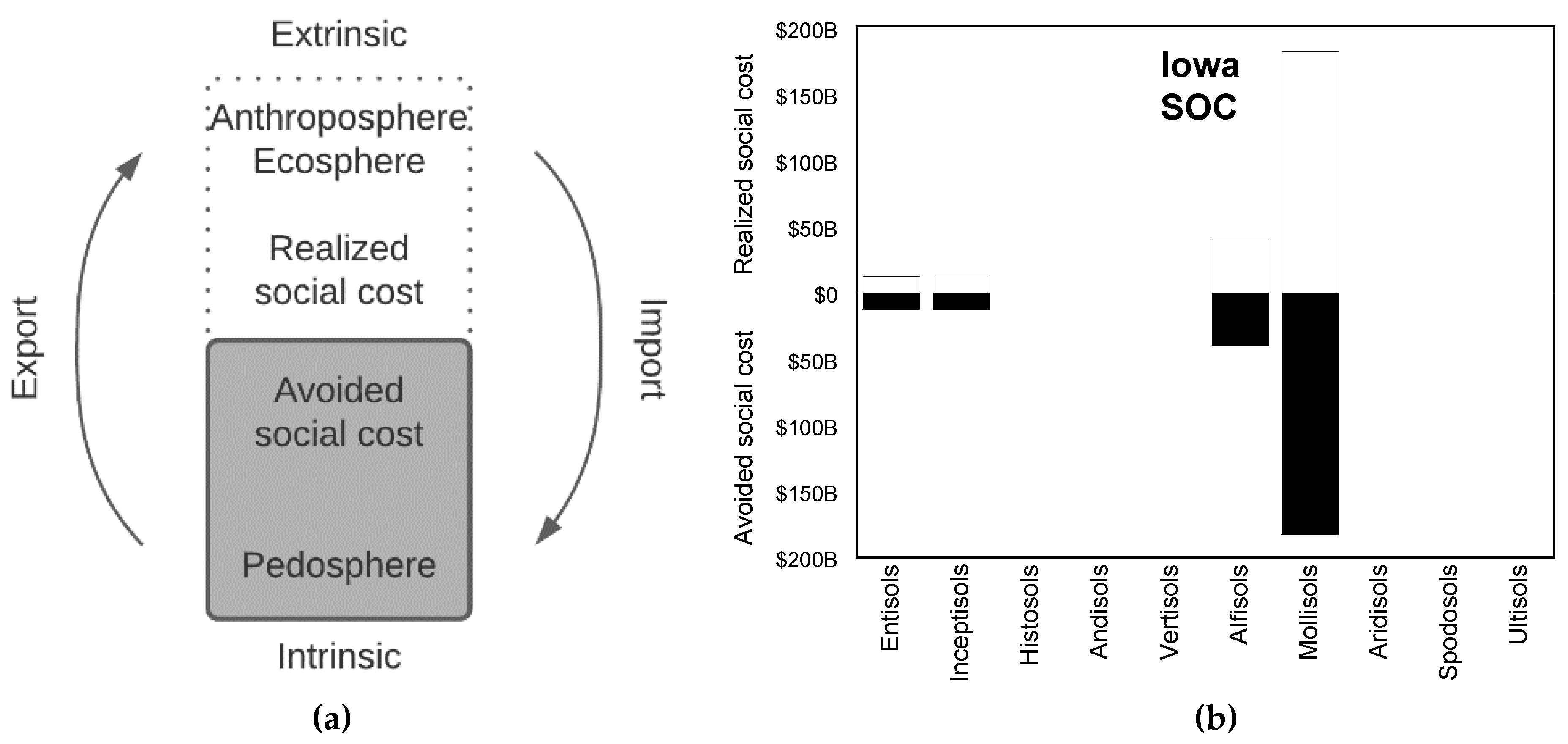
2.2. The Accounting Framework

| STOCKS | FLOWS | VALUE | ||
|---|---|---|---|---|
| Biophysical Accounts (Science-Based) | Administrative Accounts (Boundary-Based) | Monetary Accounts | Benefits/Damages | Total Value |
| Soil extent: | Administrative extent: | Ecosystem good(s) and service(s): | Sector: | Types of value: |
| Examples of valuations based on soil diversity (pedodiversity) | ||||
| Examples of valuations based on the interaction of soil diversity (pedodiversity) and the Earth’s spheres | ||||
| Soil diversity (pedodiversity), organizational hierarchy of soil systems | Administrative, organizational hierarchy | Provisioning, regulation/ maintenance and cultural | Environment, agriculture, industry, etc. | Market and non-market valuations |
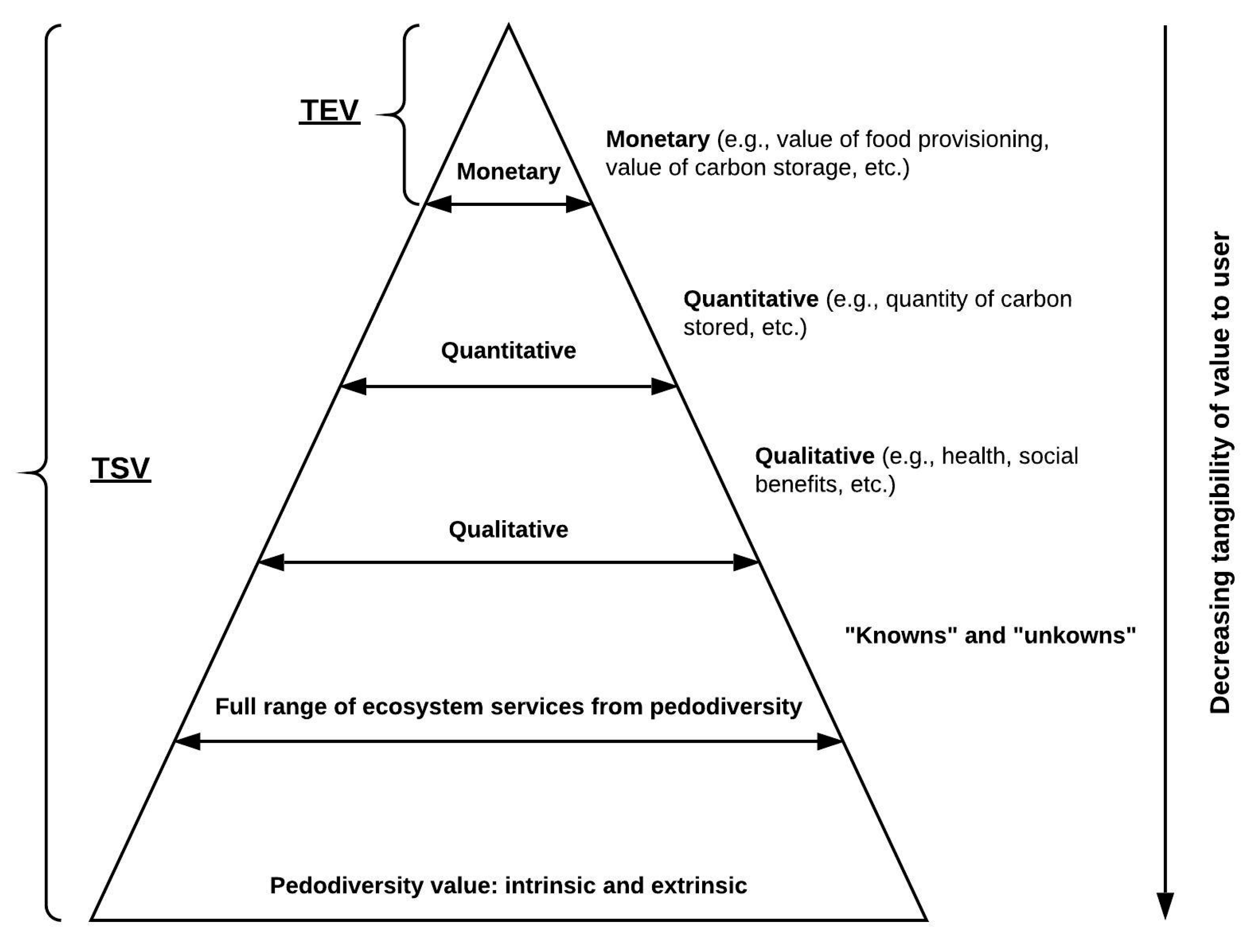
2.3. The Total Economic Value (TEV) Framework with Insurance Value
| Total Economic Value (TEV) | ||||||
| Instrumental Value (Benefits to Humans) | Intrinsic Value (Benefits to Nature) | |||||
| Use Values | Insurance | |||||
| Actual Use Values | Passive Use Values | Value | Unknown | |||
| Direct Use Value (extractive and non-extractive uses) | Indirect Use Value (functional benefits) | Altruistic Value (for others) | Bequest Value (for others) | Existence Value (for life) | The amount available to replace lost value | |
| Consumptive and non-consumptive (e.g., agriculture) | e.g., ecosystem services | e.g., preserving resource so others can use it now | e.g., preserving resource so others can use it in the future | e.g., resource preservation | e.g., buffering capacity | |
| Option Value | ||||||
| ----------------------------------------------------------- Decreasing Tangibility of Value to User ----------------------------------------------------> | ||||||
3. Results
3.1. Intrinsic Factors: Examples of Valuations Based on Pedodiversity and Ecosystem Services
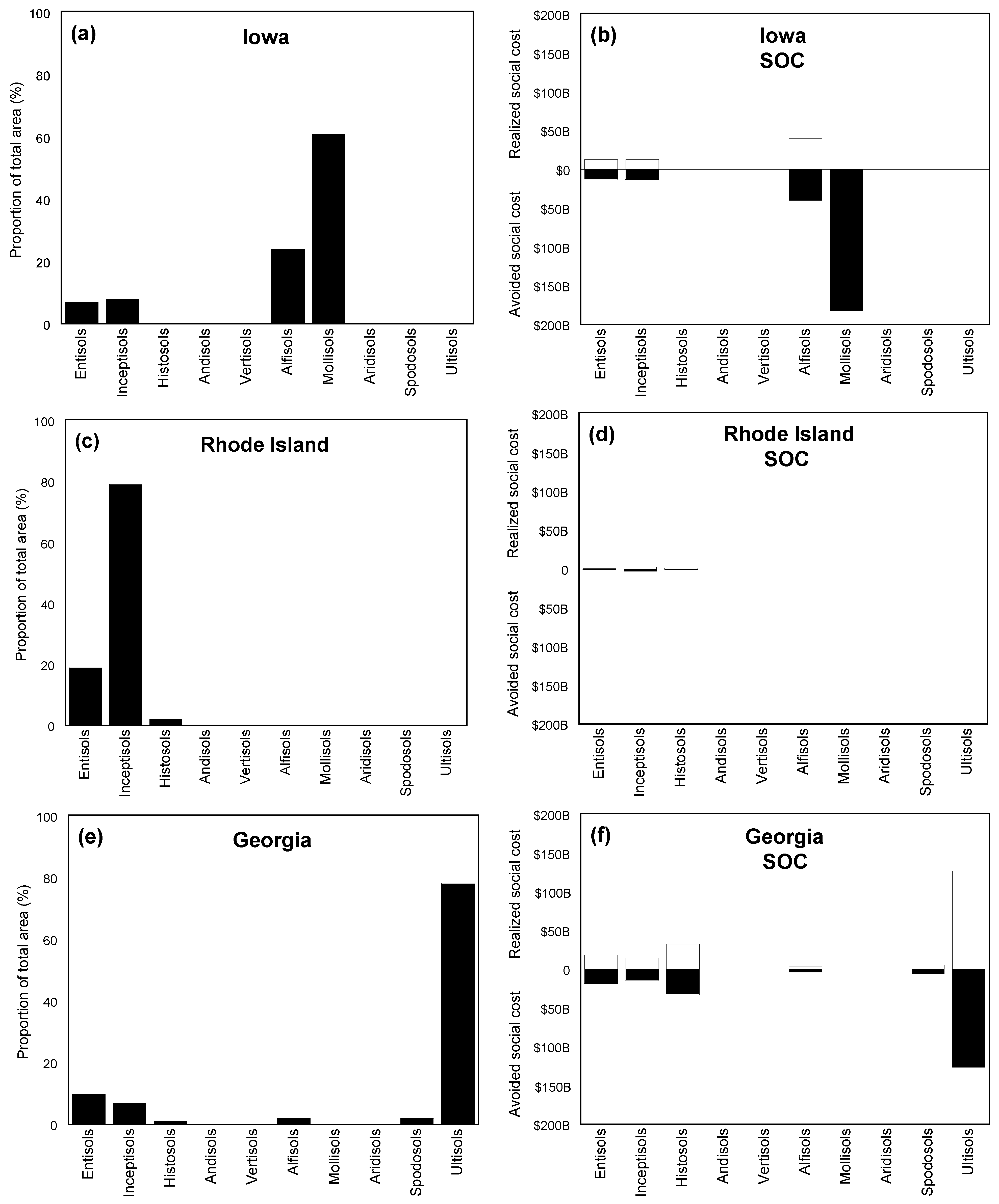
3.1.1. Examples of Taxonomic Pedodiversity and Ecosystem Services in the Contiguous U.S.
3.1.2. Examples of Genetic Pedodiversity and Ecosystem Services
3.1.3. Examples of Parametric Pedodiversity and Ecosystem Services
3.1.4. Examples of Functional Pedodiversity and Ecosystem Services
3.2. Extrinsic Factors: Examples of Monetary Valuations Based on Interaction of Soil Diversity (Pedodiversity) and the Earth’s Spheres
3.3. Pedodiversity Threats and Losses in the Contiguous U.S. in Relation to Ecosystem Services
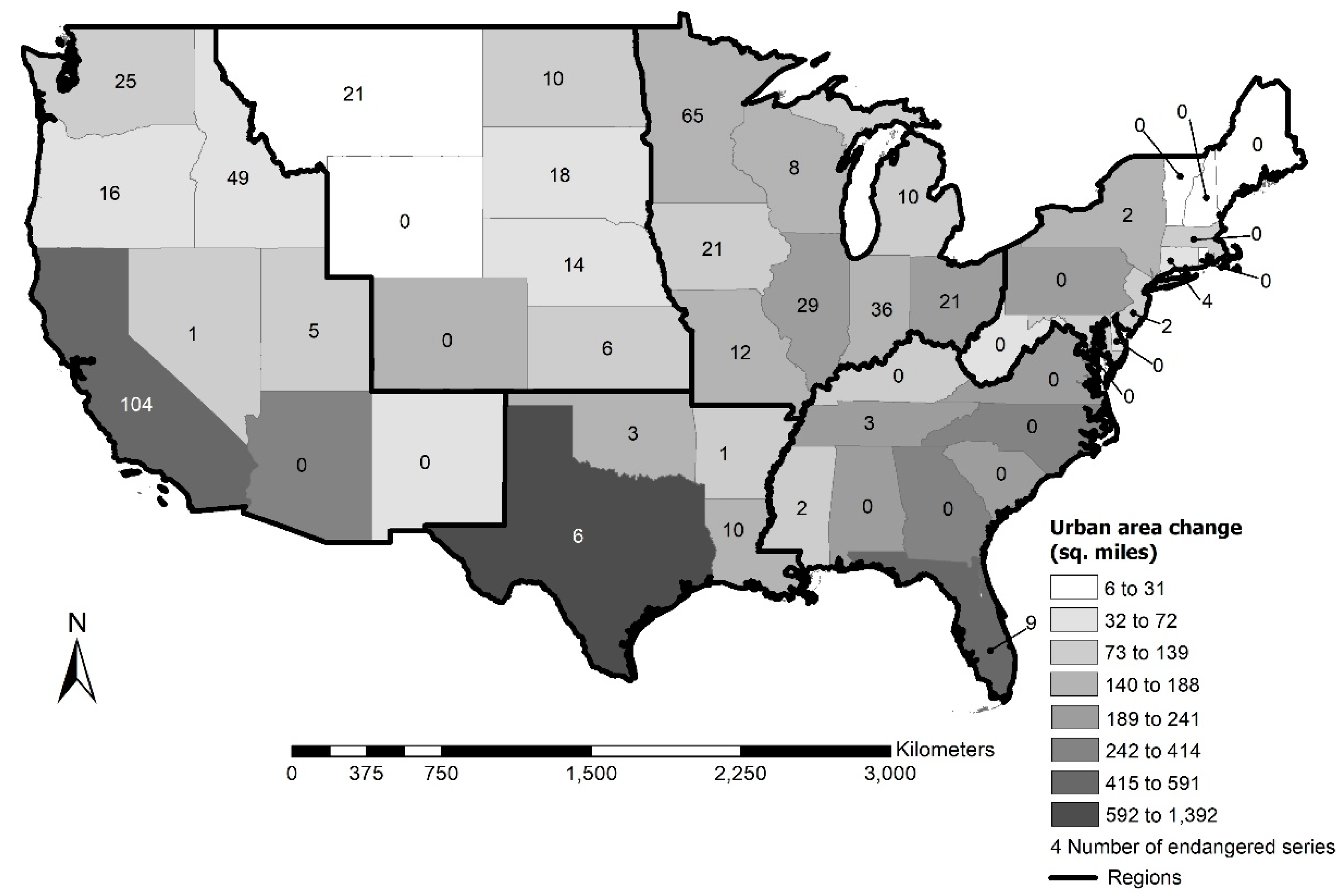
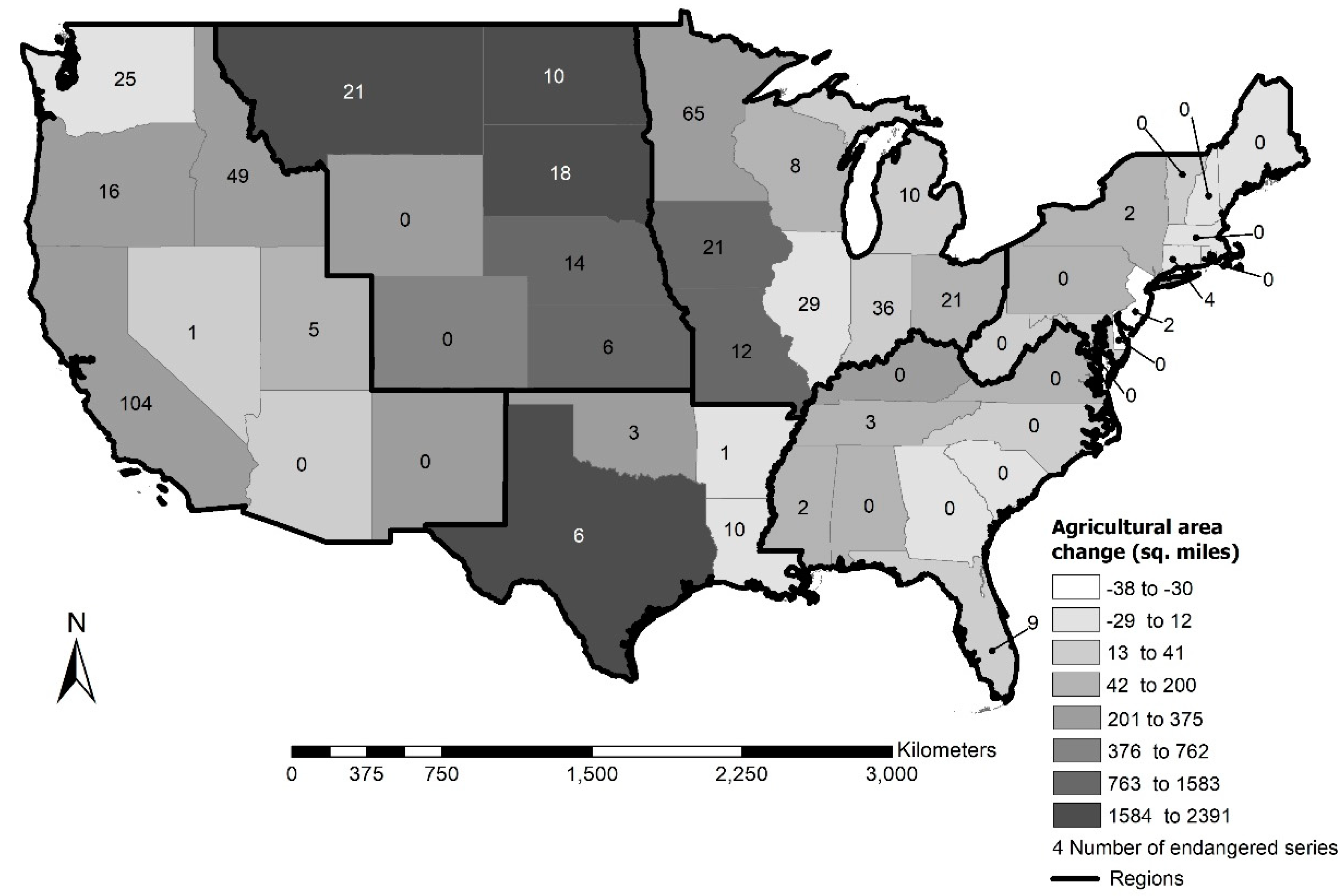
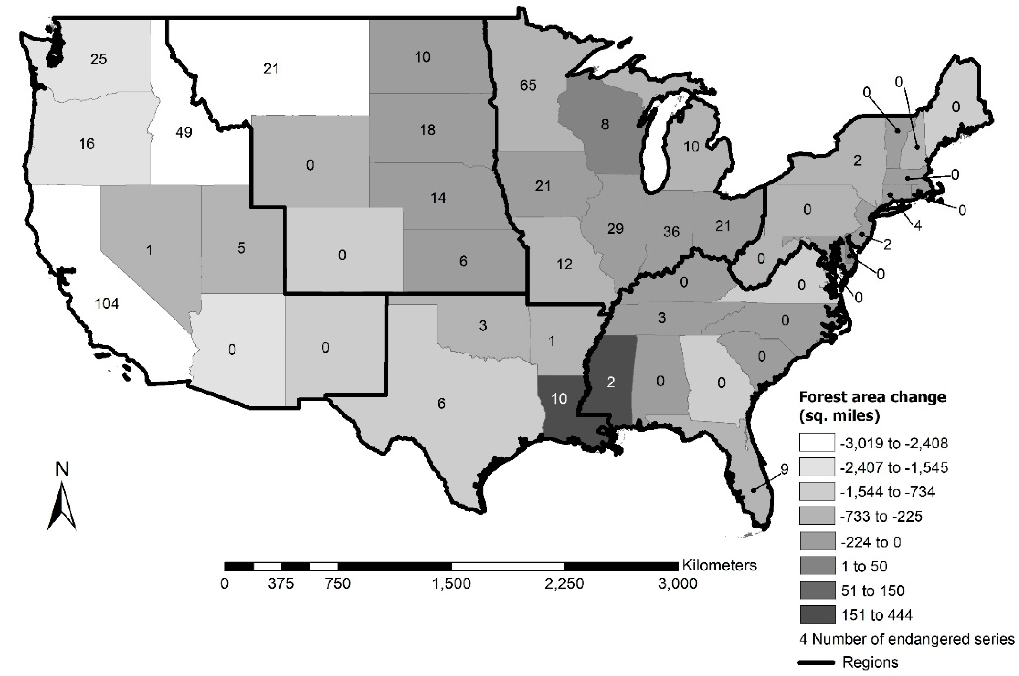
3.3.1. Land Cover Change (LCC) as a Threat to Pedodiversity
3.3.2. Climate Change as a Threat to Pedodiversity
- Biotic (e.g., increase in soil organic matter decomposition rates due to increase in temperature and precipitation [66] leading to increase in soil CO2 emissions and associated social costs);
- Abiotic (e.g., increase in soil erosion due to an increase in precipitation and extreme rainfall events [67]).
4. Discussion

5. Conclusions
Author Contributions
Funding
Acknowledgments
Conflicts of Interest
Glossary
| ED | Ecosystem disservices |
| ES | Ecosystem services |
| EPA | Environmental Protection Agency |
| SC-CO2 | Social cost of carbon emissions |
| SDGs | Sustainable Development Goals |
| SOC | Soil organic carbon |
| SIC | Soil inorganic carbon |
| SOM | Soil organic matter |
| SSURGO | Soil Survey Geographic Database |
| TEV | Total economic value |
| TSV | Total system value |
| USDA | United States Department of Agriculture |
| US | United States |
References
- Jenny, H. Factors of Soil Formation; McGraw Hill: New York, NY, USA, 1941. [Google Scholar]
- Amundson, R.; Guo, Y.; Gong, P. Soil diversity and land use in the United States. Ecosystems 2003, 6, 470–482. [Google Scholar] [CrossRef]
- Mattson, S. The constitution of the pedosphere. Ann. Agric. Coll. Swed. 1938, 5, 261–279. [Google Scholar]
- Odeh, L.O.A. In Discussion of: Ibáñez, J.J.; De-Alba, S.; Lobo, A.; Zucarello, V. Pedodiversity and global soil pattern at coarse scales. Geoderma 1998, 83, 203–205. [Google Scholar]
- Ibáñez, J.J.; De-Alba, S.; Lobo, A.; Zucarello, V. Pedodiversity and global soil patterns at coarse scales (with Discussion). Geoderma 1998, 83, 171–214. [Google Scholar] [CrossRef] [Green Version]
- Phillips, J.D. The relative importance of intrinsic and extrinsic factors in pedodiversity. Ann. Am. Assoc. Geogr. 2001, 91, 609–621. [Google Scholar] [CrossRef]
- Dobrovolskii, G.V. Dokuchaev’s language as a reflection of his broad vision and literary talent. Eurasian Soil Sci. 2007, 40, 1008–1015. [Google Scholar] [CrossRef]
- Fridland, V.M. Pattern of the Soil Cover; John Wiley & Sons: Hoboken, NJ, USA, 1977; ISBN 13-978-0470991671. [Google Scholar]
- Hole, F.D.; Campbell, J.B. Soil Landscape Analysis; Rowman and Littlefield: Lanham, MD, USA, 1985; 214p, ISBN 13 978-0865981409. [Google Scholar]
- McBratney, A.B. On variation, uncertainty and informatics in environmental soil management. Aust. J. Soil Res. 1992, 30, 913–935. [Google Scholar] [CrossRef]
- Ibáñez, J.J.; De-Alba, S.; Bermúdez, F.F.; García-Álvarez, A. Pedodiversity: Concepts and measures. Catena 1995, 24, 215–232. [Google Scholar] [CrossRef]
- Mikhailova, E.A.; Post, C.J.; Schlautman, M.A.; Post, G.C.; Zurqani, H.A. The business side of ecosystem services of soil systems. Earth 2020, 1, 2. [Google Scholar] [CrossRef]
- Ibáñez, J.J.; Saldaña, A.; Olivera, D. Biodiversity and pedodiversity: A matter of coincidence? SJSS 2012, 2, 8–12. [Google Scholar] [CrossRef]
- Guo, Y.; Amundson, R.; Gong, P.; Ahrens, R. Taxonomic structure, distribution, and abundance of the soils in the USA. SSSAJ 2003, 67, 1507–1516. [Google Scholar] [CrossRef]
- Soil Survey Staff. A Basic System of Soil Classification for Making and Interpreting Soil Surveys. In Soil Taxonomy; Agricultural Handbook 436; US Department of Agriculture, Natural Resources Conservation Service: Washington, DC, USA, 1999. [Google Scholar]
- Adhikari, K.; Hartemink, A.E. Linking soils to ecosystem services—A global review. Geoderma 2016, 262, 101–111. [Google Scholar] [CrossRef]
- Comerford, N.B.; Franzlubbers, A.J.; Stromberger, M.E.; Morris, L.; Markewitz, D.; Moore, R. Assessment and evaluation of soil ecosystem services. Soil Horiz. 2013, 54, 1–14. [Google Scholar] [CrossRef] [Green Version]
- Baveye, P.C.; Baveye, J.; Gowdy, J. Soil “ecosystem” services and natural capital: Critical appraisal of research on uncertain ground. Front. Environ. Sci. 2016, 4, 41. [Google Scholar] [CrossRef]
- Millennium Ecosystem Assessment (MEA). Ecosystems and Human Well-Being: Synthesis; Island Press: Washington, DC, USA, 2005. [Google Scholar]
- Bartkowski, B.; Bartke, S.; Helming, K.; Paul, C.; Techen, A.; Hansjürgens, B. Potential of the economic valuation of soil-based ecosystem services to inform sustainable soil management and policy. Peer J. 2020, 8, e8749. [Google Scholar] [CrossRef] [Green Version]
- Bartkowski, B. Are diverse ecosystems more valuable? Economic value of biodiversity as result of uncertainty and spatial interactions in ecosystem service provision. Ecosyst. Serv. 2017, 24, 50–57. [Google Scholar] [CrossRef]
- De Groot, R.; Jax, K.; Harrison, P. Links between biodiversity and ecosystem services. In OpenNESS Ecosystem Services Reference Book; Potschin, M., Jax, K., Eds.; EC FP7 Grant Agreement No. 308428; 2016; Available online: http://www.openness-project.eu/library/reference-book (accessed on 10 October 2020).
- Schnediders, A.; Van Daele, T.; Van Landuyt, W.; Van Reeth, W. Biodiversity and ecosystem services: Complementary approaches for ecosystem management? Ecol. Indic. 2012, 21, 123–133. [Google Scholar] [CrossRef]
- Cardinale, B.; Duffy, J.; Gonzalez, A.; Hooper, D.; Perrings, C.; Venail, P.; Narwani, A.; Mace, G.; Tilman, D.; Naeem, S.; et al. Biodiversity loss and its impact on humanity. Nature 2012, 486, 59–67. [Google Scholar] [CrossRef]
- Stephenson, J. Business, biodiversity and ecosystem services: Policies priorities for engaging business to improve health of ecosystems and conserve biodiversity. In Proceedings of the 28th Round Table on Sustainable Development, Telangana, India, 16 October 2012. [Google Scholar]
- Chandler, R.D.; Mikhailova, E.A.; Post, C.J.; Moysey, S.M.J.; Schlautman, M.A.; Sharp, J.L.; Motallebi, M. Integrating soil analyses with frameworks for ecosystem services and organizational hierarchy of soil systems. Commun. Soil Sci. Plant Anal. 2018, 49, 1835–1843. [Google Scholar] [CrossRef]
- Soil Survey Staff, Natural Resources Conservation Service, United States Department of Agriculture. Soil Survey Geographic (SSURGO) Database. Available online: https://www.nrcs.usda.gov/wps/portal/nrcs/detail/soils/survey/?cid=nrcs142p2_053627 (accessed on 10 September 2020).
- Clarivate Analytics. Web of Science. Subscription-Based Website. 2020. Available online: https://clarivate.com/tag/web-of-science/ (accessed on 21 September 2020).
- Pavan, A.L.R.; Ometto, A.R. Ecosystem services in life cycle assessment: A novel conceptual framework for soil. Sci. Total Environ. 2018, 643, 1337–1347. [Google Scholar] [CrossRef] [PubMed]
- Groshans, G.R.; Mikhailova, E.A.; Post, C.J.; Schlautman, M.A. Accounting for soil inorganic carbon in the ecosystem services framework for the United Nations sustainable development goals. Geoderma 2018, 324, 37–46. [Google Scholar] [CrossRef] [Green Version]
- Nimmo-Bell. MAF Biosecurity New Zealand. TEV for Biodiversity; Nimmo-Bell: Wellington, New Zealand, 2011; Available online: http://www.nimmo-bell.co.nz/pdf/ManualRev29411.pdf (accessed on 10 October 2020).
- Van Zyl, S.; Au, J. The Start of a Conversation on the Value of New Zealand’s Natural Capital; Living Standards Series: Discussion Paper 18/03; Office of the Chief Economic Advisor: Wellington, New Zealand, 2018. Available online: https://www.treasury.govt.nz/sites/default/files/2018-02/dp18-03.pdf (accessed on 10 October 2020).
- Soil Survey Staff; Natural Resources Conservation Service; United States Department of Agriculture. Web Soil Survey. Available online: http://websoilsurvey.sc.egov.usda.gov/ (accessed on 16 October 2020).
- Soil Science Society of America. Penistaja New Mexico State Soil. State Soil Booklets. Available online: https://www.soils4teachers.org/files/s4t/k12outreach/nm-state-soil-booklet.pdf (accessed on 14 October 2020).
- Mikhailova, E.A.; Groshans, G.R.; Post, C.J.; Schlautman, M.A.; Post, G.C. Valuation of soil organic carbon stocks in the contiguous United States based on the avoided social cost of carbon emissions. Resources 2019, 8, 153. [Google Scholar] [CrossRef] [Green Version]
- Mikhailova, E.A.; Groshans, G.R.; Post, C.J.; Schlautman, M.A.; Post, G.C. Valuation of total soil carbon stocks in the contiguous United States based on the avoided social cost of carbon emissions. Resources 2019, 8, 157. [Google Scholar] [CrossRef] [Green Version]
- Mikhailova, E.A.; Post, C.J.; Schlautman, M.A.; Post, G.C.; Zurqani, H.A. Determining farm-scale site-specific monetary values of “soil carbon hotspots” based on avoided social costs of CO2 emissions. Cogent Environ. Sci. 2020, 6:1, 1817289. [Google Scholar] [CrossRef]
- Brevik, E.C.; Hartemink, A.E. Soil maps of the United States of America. Soil Sci. Soc. Am. 2013, 77, 1117–1132. [Google Scholar] [CrossRef] [Green Version]
- Guo, Y.; Amundson, R.; Gong, P.; Yu, Q. Quantity and spatial variability of soil carbon in the conterminous United States. Soil Sci. Soc. Am. J. 2006, 70, 590–600. [Google Scholar] [CrossRef] [Green Version]
- Hartemink, A.E.; Zhang, Y.; Bockheim, J.G.; Curi, N.; Silva, S.H.G.; Grauer-Gray, J.; Lowe, D.J.; Krasilnikov, P. Soil Horizon Variation: A review. Adv. Agron. 2020, 160. [Google Scholar] [CrossRef]
- Mikhailova, E.A.; Bryant, R.B.; Vassenev, I.I.; Schwager, S.J.; Post, C.J. Cultivation effects on soil organic carbon and total nitrogen at depth in the Russian Chernozem. Soil Sci. Soc. Am. J. 2000, 64, 738–745. [Google Scholar] [CrossRef]
- Bullock, C.H.; Collier, M.J.; Convery, F. Peatlands, their economic value and priorities for their future management—The example of Ireland. Land Use Policy 2012, 29, 921–928. [Google Scholar] [CrossRef]
- Anisimov, O.A. Potential feedback of thawing permafrost to the global climate system through methane emission. Environ. Res. Lett. 2007, 2, 045016. [Google Scholar] [CrossRef]
- Singh, B.; Schulze, D.G. Soil minerals and plant nutrition. Nat. Educ. Knowl. 2015, 6, 1–10. [Google Scholar]
- Zurqani, H.A.; Mikhailova, E.A.; Post, C.J.; Schlautman, M.A.; Elhawej, A.R. A review of Libyan soil databases for use within an ecosystem services framework. Land 2019, 8, 82. [Google Scholar] [CrossRef] [Green Version]
- Groshans, G.R.; Mikhailova, E.A.; Post, C.J.; Schlautman, M.A.; Zhang, L. Determining the value of soil inorganic carbon stocks in the contiguous United States based on the avoided social cost of carbon emissions. Resources 2019, 8, 119. [Google Scholar] [CrossRef] [Green Version]
- Mikhailova, E.A.; Post, C.J.; Gerard, P.D.; Schlautman, M.A.; Cope, M.P.; Groshans, G.R.; Stiglitz, R.Y.; Zurqani, H.A.; Galbraith, J.M. Comparing field sampling and soil survey database for spatial heterogeneity in surface soil granulometry: Implications for the ecosystem services assessment. Front. Environ. Sci. 2019, 7, 128. [Google Scholar] [CrossRef]
- Oliver, M.A.; Gregory, P.J. Soil, food security and human health: A review. Eur. J. Soil Sci. 2015, 66, 257–276. [Google Scholar] [CrossRef]
- Merrill, D.; Leatherby, L. Here’s how America uses its land. Bloomberg. 2018. Available online: https://www.bloomberg.com/graphics/2018-us-land-use/ (accessed on 14 October 2020).
- Schlesinger, W.H.; Amundson, R. Managing for soil carbon sequestration: Let’s get realistic. Glob. Chang. Biol. 2019, 25, 386–389. [Google Scholar] [CrossRef] [Green Version]
- EPA. The Social Cost of Carbon. EPA Fact Sheet. 2016. Available online: https://19january2017snapshot.epa.gov/climatechange/social-cost-carbon_.html (accessed on 15 March 2019).
- Mikhailova, E.A.; Zurqani, H.A.; Post, C.J.; Schlautman, M.A. Assessing ecosystem services of atmospheric calcium and magnesium deposition for potential soil inorganic carbon sequestration. Geosciences 2020, 10, 200. [Google Scholar] [CrossRef]
- Duncombe, J. The ticking time bomb of Arctic permafrost. Eos 2020, 101. [Google Scholar] [CrossRef]
- Restuccia, F.; Huang, X.; Rein, G. Self-ignition of natural fuels: Can wildfires of carbon-rich soil start by self-heating? Fire Saf. J. 2017, 91, 828–834. [Google Scholar] [CrossRef]
- Borrelli, P.; Robinson, D.A.; Panagos, P.; Lugato, E.; Yang, J.E.; Alewell, C.; Wuepper, D.; Montarella, L.; Ballabio, C. Land use and climate change impacts on global soil erosion by water (2015–2070). PNAS 2020, 117, 21994–22001. [Google Scholar] [CrossRef]
- Pavao-Zuckerman, M.A. The nature of urban soils and their role in ecological restoration in cities. Restor. Ecol. 2008, 16, 642–649. [Google Scholar] [CrossRef]
- Vasenev, V.I.; Van Oudenhoven, A.P.E.; Romzaykina, O.N.; Hajiaghaeva, R.A. The ecological functions and ecosystem services of urban and technogenic soils: From theory to practice (A review). Eurasian Soil Sci. 2018, 51, 1119–1132. [Google Scholar] [CrossRef] [Green Version]
- Grunewald, K.; Bastian, O. Special issue: Maintaining ecosystem services to support urban needs. Sustainability 2017, 9, 1647. [Google Scholar] [CrossRef] [Green Version]
- Groshans, G.R.; Mikhailova, E.A.; Post, C.J.; Schlautman, M.A.; Zurqani, H.A.; Zhang, L. Assessing the value of soil inorganic carbon for ecosystem services in the contiguous United States based on liming replacement costs. Land 2018, 7, 149. [Google Scholar] [CrossRef] [Green Version]
- Wikipedia. List of States and Territories of the United States by Population. Available online: https://en.wikipedia.org/wiki/List_of_states_and_territories_of_the_United_States_by_population (accessed on 22 October 2020).
- United States Summary. 2010 Census of Population and Housing, Population and Housing Unit Counts; CPH-2-5; U.S. Government Printing Office, U.S. Census Bureau: Washington, DC, USA, 2012; p. 42. Available online: https://www2.census.gov/library/publications/decennial/2010/cph-2/cph-2-1.pdf (accessed on 10 October 2020).
- Goldenberg, R.; Kalantari, Z.; Cvetkovic, V.; Mörtberg, U.; Deal, B.; Destouni, G. Distinction, quantification and mapping of potential and realized supply-demand of flow-dependent ecosystem services. Sci. Total Environ. 2017, 593–594, 599–609. [Google Scholar] [CrossRef]
- Hewes, L. The Suitcase Farming Frontier: A study in the Historical Geography of the Central Great Plains; University of Nebraska Press: Linkoln, NE, USA, 1974; 281p. [Google Scholar]
- Lee, J.A.; Gill, T.E. Multiple causes of wind erosion in the Dust Bowl. Aeolian Res. 2015, 19, 15–36. [Google Scholar] [CrossRef]
- Wentland, S.A.; Ancona, Z.H.; Bagstad, K.J.; Boyd, J.; Hass, J.L.; Gindelsky, M.; Moulton, J.G. Accounting for land in the United States: Integrating physical land cover, land use, and monetary valuation. Ecosyst. Serv. 2020, 46, 101178. [Google Scholar] [CrossRef]
- Lu, M.; Zhou, X.; Yang, Q.; Li, H.; Luo, Y.; Fang, C.; Chen, J.; Yang, X.; Li, B. Responses of ecosystem carbon cycle to experimental warming: A meta-analysis. Ecology 2013, 94, 726–738. [Google Scholar] [CrossRef] [PubMed]
- Nearing, M.A.; Pruski, F.F.; O’Neal, M.R. Expected climate change impacts on soil erosion rates: A review. J. Soil Water Conserv. 2004, 59, 43–50. [Google Scholar]
- Chen, C.; McCarl, B.; Chang, C. Climate change, sea level rise and rice: Global market implications. Clim. Chang. 2012, 110, 543–560. [Google Scholar] [CrossRef] [Green Version]
- Walthall, C.L.; Hatfield, J.; Backlund, P.; Lengnick, L.; Marshall, E.; Walsh, M.; Adkins, S.; Aillery, M.; Ainsworth, E.A.; Ammann, C.; et al. Climate Change and Agriculture in the United States: Effects and Adaptation; USDA Technical Bulletin 1935; USDA: Washington, DC, USA, 2012; 186p.
- Reilly, J.; Tubiello, F.; McCarl, B.; Abler, D.; Darwin, R.; Fuglie, K.; Hollinger, S.; Izarralde, C.; Jagtap, S.; Jones, J.; et al. Agriculture and climate change: New results. Clim. Chang. 2003, 57, 43–69. [Google Scholar] [CrossRef]
- Amundson, R.; Berhe, A.A.; Hopmans, J.W.; Olson, C.; Sztein, A.E.; Sparks, D.L. Soil and human security in the 21st century. Science 2015, 348. [Google Scholar] [CrossRef] [PubMed] [Green Version]
- Pascual, U.; Termansen, M.; Hedlund, K.; Brussaard, L.; Faber, J.H.; Foudi, S.; Lemanceau, P.; Jørgensen, S.L. On the value of soil biodiversity and ecosystem services. Ecosyst. Serv. 2015, 15, 11–18. [Google Scholar] [CrossRef]
- Mace, G.M.; Norris, K.; Fitter, A.H. Biodiversity and ecosystem services: A multilayered relationship. Trends Ecol. Evol. 2012, 27, 19–26. [Google Scholar] [CrossRef]
- Gerasimova, M.I. Chinese Soil Taxonomy: Between the American and the International classification systems. Eurasian J. Soil Sci. 2010, 43, 945–949. [Google Scholar] [CrossRef]
- Tilman, D.; Lehman, C.L.; Bristow, C.E. Diversity-stability relationships: Statistical inevitability or ecological consequence? Am. Nat. 1998, 151, 277–282. [Google Scholar] [CrossRef] [PubMed]
- Gantioler, S.; Rayment, M.; Bassi, S.; Kettunen, M.; McConville, A.; Landgrebe, R.; Gerdes, H.; ten Brink, P. Costs and Socio-Economic Benefits Associated with the Natura 2000 Network; Final report to the European Commission; DG Environment on Contract ENV.B.2/SER/2008/0038; Institute for European Environmental Policy/GHK /Ecologic: Brussels, Belgium, 2010. [Google Scholar]
- Wall, D.H.; Nielsen, U.N. Biodiversity and ecosystem services: Is it the same below ground? Nat. Educ. Knowl. 2012, 3, 8. [Google Scholar]
- Vos, C.C.; Grashof-Bokdam, C.J.; Opdam, P.F.M. Biodiversity and Ecosystem Services: Does Species Diversity Enhance Effectiveness and Reliability? A Systematic Literature Review; WOT-Technical Report 25; Statutory Research Tasks Unit for Nature and the Environment (WOT Natuur and Milieu): Wageningen, The Netherlands, 2014; 64p, ISSN 2352-2739. [Google Scholar]
- Lal, R. Soils and sustainable agriculture. A review. Agron. Sustain. Dev. 2008, 28, 57–64. [Google Scholar] [CrossRef]
- Power, A.G. Ecosystem services and agriculture: Tradeoffs and synergies. Phil. Trans. R. Soc. B 2010, 365, 2959–2971. [Google Scholar] [CrossRef]
- Cordell, D.; Drangert, J.O.; White, S. The story of phosphorus: Global food security and food for thought. Glob. Environ. Chang. 2009, 19, 292–305. [Google Scholar] [CrossRef]
- Mikhailova, E.A.; Post, G.C.; Cope, M.P.; Post, C.J.; Schlautman, M.A.; Zhang, L. Quantifying and mapping atmospheric potassium deposition for soil ecosystem services assessment in the United States. Front. Environ. Sci. 2019, 7, 74. [Google Scholar] [CrossRef]
- Świader, M.; Lin, D.; Szewrański, S.; Kazak, J.K.; Iha, K.; van Hoof, J.; Belčáková, I.; Altiok, S. The application of ecological footprint and biocapacity for environmental carrying capacity assessment: A new approach for European cities. Environ. Sci. Policy 2020, 105, 56–74. [Google Scholar] [CrossRef]
- Raffaelli, D. How extinction patterns affect ecosystems. Science 2004, 306, 1141–1142. [Google Scholar] [CrossRef] [PubMed] [Green Version]
- Brady, N.C.; Weil, R.R. The Nature and Properties of Soils, 13rd ed.; Pearson Education: London, UK, 2002. [Google Scholar]
- Pastick, N.J.; Torre Jorgenson, M.; Wylie, B.K.; Nield, S.J.; Johnson, K.D.; Finley, A.O. Distribution of near-surface permafrost in Alaska: Estimates of present and future conditions. Remote Sens. Environ. 2015, 168, 301–315. [Google Scholar] [CrossRef] [Green Version]
- Leifeld, J.; Menichetti, L. The underappreciated potential of peatlands in global climate change mitigation strategies. Nat. Commun. 2018, 9, 1071. [Google Scholar] [CrossRef] [PubMed] [Green Version]
- Hansjürgens, B.; Lienkamp, A.; Möckel, S. Justifying soil protection and sustainable soil management: Creation-ethical, legal and economic considerations. Sustainability 2018, 10, 3807. [Google Scholar] [CrossRef] [Green Version]
- Guerry, A.D.; Polasky, S.; Lubchenco, J.; Chaplin-Kramer, R.; Daily, G.C.; Griffin, R.; Ruckelshaus, M.; Bateman, I.J.; Duraiappah, A.; Elmqvist, T.; et al. Natural capital and ecosystem services informing decisions: From promise to practice. PNAS 2015, 112, 7348–7355. [Google Scholar] [CrossRef] [Green Version]
- Jones, C.A.; DiPinto, L. The role of ecosystem services in USA natural resources liability litigation. Ecosyst. Serv. 2018, 29, 333–351. [Google Scholar] [CrossRef]
- Zhu, Y.; Meharg, A. Protecting global soil resources for ecosystem services. Ecosyst. Health Sustain. 2015, 1, 11. [Google Scholar] [CrossRef]
- McBratney, A.; Field, D.J.; Koch, A. The dimensions of soil security. Geoderma 2014, 213, 203–213. [Google Scholar] [CrossRef] [Green Version]
- Ibáñez, J.J. Diversity of Soils; Oxford University Press: Oxford, UK, 2017. [Google Scholar] [CrossRef]
- Bach, E.M.; Ramirez, K.S.; Fraser, T.D.; Wall, D.H. Soil biodiversity integrates solutions for a sustainable future. Sustainability 2020, 12, 2662. [Google Scholar] [CrossRef] [Green Version]
- Dazzi, C.; Papa, G.L. Soil genetic erosion: New conceptual developments in soil security. Int. Soil Water Conserv. Res. 2019, 7, 317–324. [Google Scholar] [CrossRef]
- Chen, J.; Zhang, X.-L.; Gong, Z.-T.; Wang, J. Pedodiversity: A controversial concept. J. Geogr. Sci. 2001, 11, 110–116. [Google Scholar] [CrossRef]
- Asah, S.T.; Guerry, A.D.; Blahna, D.J.; Lawler, J.J. Perception, acquisition and use of ecosystem services: Human behavior, and ecosystem management and policy implications. Ecosyst. Serv. 2014, 10, 180–186. [Google Scholar] [CrossRef]


| Types of Soil Diversity (Pedodiversity) | Examples |
|---|---|
| Taxonomic (diversity of soil classes) | USDA Soil Taxonomy (e.g., soil order, series) |
| Genetic (diversity of genetic horizons) | A, B, etc. |
| Parametric (diversity of soil properties) | Soil organic matter (SOM), calcium carbonate (CaCO3), etc. |
| Functional (soil behavior under different use) | Interpretive models to predict soil behavior |
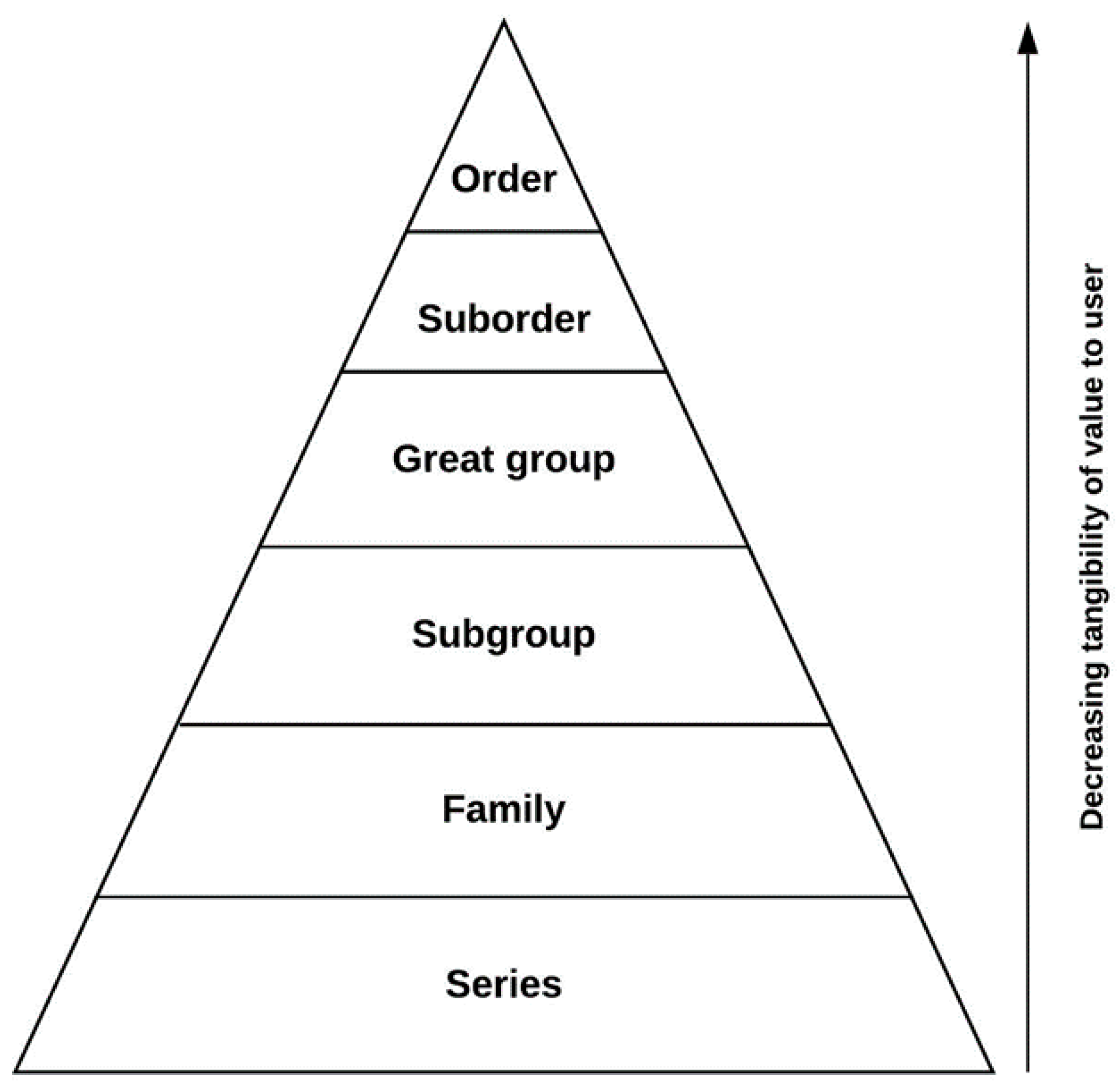
| Taxonomic Category | Explanation | Example | Increase in Specificity |
|---|---|---|---|
| Order | Highest category, diagnostic horizons | Ultisols |  |
| Suborder | The difference in moisture regimes | Udults | |
| Great Group | Presence of key horizons | Hapludults | |
| Subgroup | Proximity to “central concept” | Typic Kanhapludults | |
| Family | Particle-size classes and their substitutes | fine | |
| Human-altered and human-transported material classes | |||
| Mineralogy classes | kaolinitic | ||
| Cation-exchange activity classes (CEC/% clay) | |||
| Calcareous and reaction classes | |||
| Soil temperature classes | thermic | ||
| Soil depth classes | |||
| Rupture-resistance classes | |||
| Classes of coatings on sands | |||
| Classes of permanent cracks | |||
| Series | Smallest unit | Cecil |
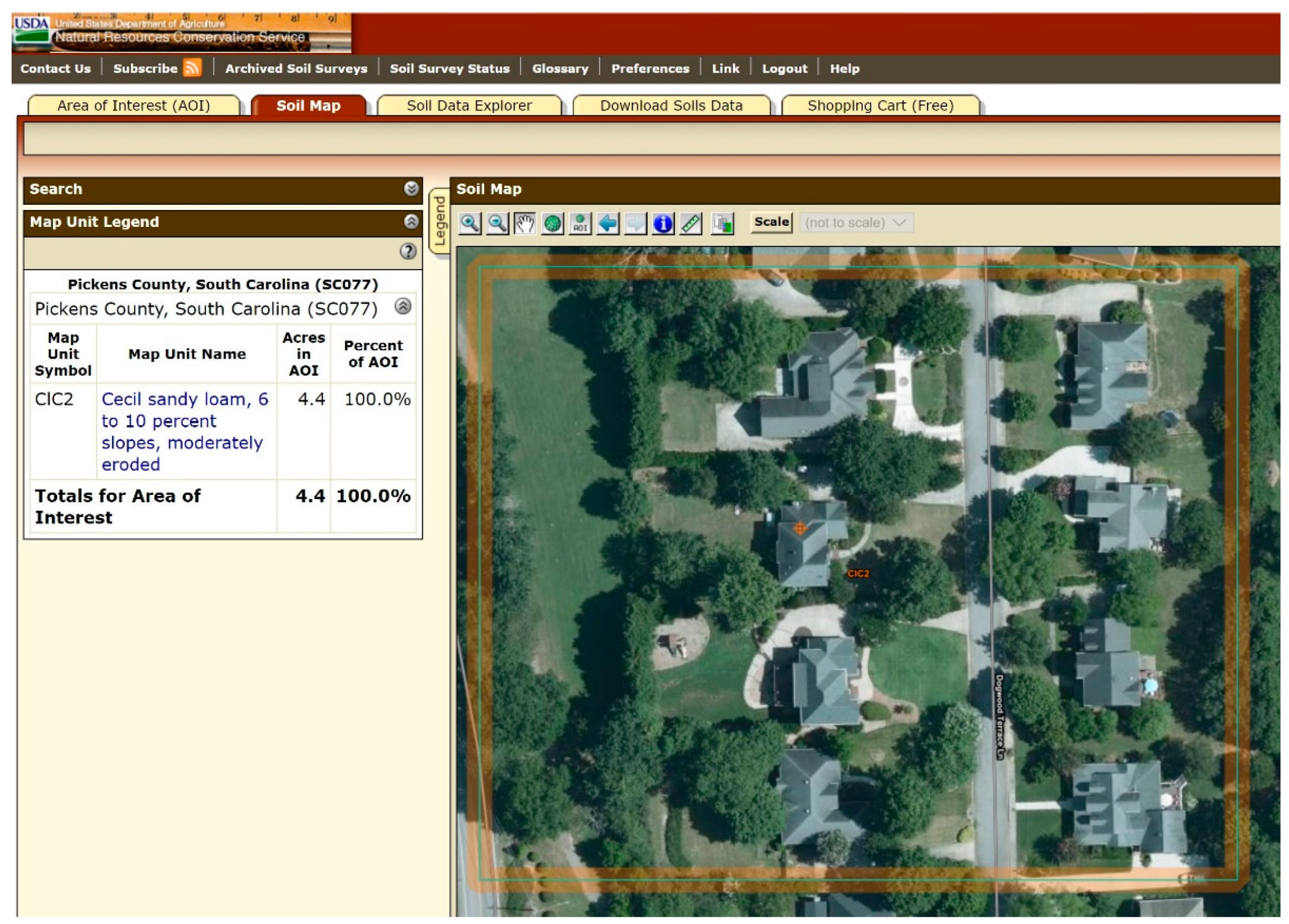
| Map Symbol and Soil Name | Depth | Sand | Silt | Clay | Organic Matter |
|---|---|---|---|---|---|
| In | Pct | Pct | Pct | Pct | |
| ClC2-Cecil sandy loam, 6 to 10 percent slopes, moderately eroded | 0-5 | 59-70-75 | 10-20-35 | 5-10-15 | 0.5-0.5-1.0 |
| 5-54 | 15-30-40 | 6-16-26 | 35-54-59 | 0.0-0.1-0.5 | |
| 54-80 | 35-40-50 | 17-27-40 | 20-33-34 | 0.0-0.1-0.5 |
| Stocks | Ecosystem Services | |||
|---|---|---|---|---|
| Soil Order | General Characteristics and Constraints | Provisioning | Regulation/Maintenance | Cultural |
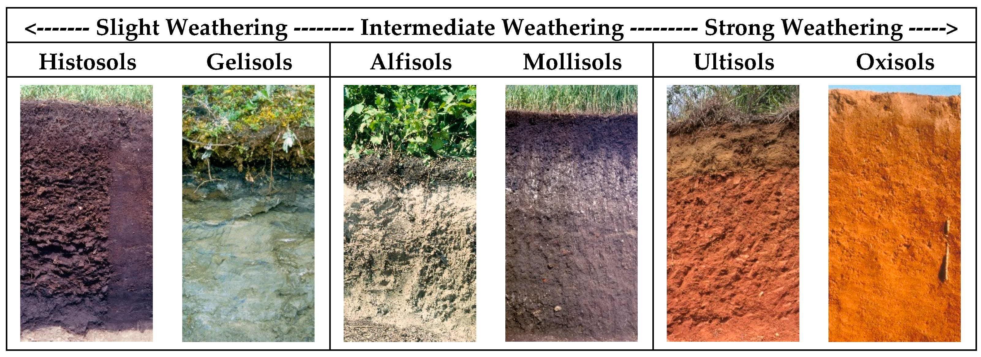
| Slight Weathering | ||||
| Entisols | Embryonic soils with ochric epipedon | x | x | x |
| Inceptisols | Young soils with ochric or umbric epipedon | x | x | x |
| Histosols | Organic soils with ≥20% of organic carbon | x | x | x |
| Gelisols | Frozen soils with permafrost | x | x | x |
| Andisols | Volcanic soils | x | x | x |
| Intermediate Weathering | ||||
| Aridisols | Dry soils. Common in desert areas | x | x | x |
| Vertisols | Soils with swelling clays | x | x | x |
| Alfisols | Clay-enriched B horizon with B.S. ≥ 35% | x | x | x |
| Mollisols | Carbon-enriched soils with B.S. ≥ 50% | x | x | x |
| Strong Weathering | ||||
| Spodosols | Coarse-textured soils with albic and spodic horizons | x | x | x |
| Ultisols | Highly leached soils with B.S. < 35% | x | x | x |
| Oxisols | Highly weathered soils rich in Fe and Al oxides | x | x | x |
| Soil Order | Suborders | Great Groups | Subgroups | Series | Series Density |
|---|---|---|---|---|---|
| Slight Weathering | |||||
| Entisols | 25 | 56 | 246 | 3700 | 3.5 |
| Inceptisols | 26 | 67 | 386 | 3610 | 4.6 |
| Histosols | 7 | 25 | 73 | 334 | 3.1 |
| Gelisols * | 2 | 2 | 2 | 2 | - |
| Andisols | 13 | 26 | 90 | 642 | 9.3 |
| Intermediate Weathering | |||||
| Aridisols | 17 | 44 | 283 | 2374 | 2.9 |
| Vertisols | 7 | 31 | 101 | 394 | 3.0 |
| Alfisols | 14 | 49 | 331 | 3242 | 2.5 |
| Mollisols | 23 | 55 | 422 | 5569 | 2.8 |
| Strong Weathering | |||||
| Spodosols | 9 | 26 | 92 | 591 | 2.4 |
| Ultisols | 9 | 27 | 107 | 1091 | 1.3 |
| Oxisols | - | - | - | - | - |
| Totals | 65 | 317 | 2026 | 19,602 | 2.7 |
| LRRs | Orders | Suborders | Great Groups | Subgroups | Series | Series Density |
|---|---|---|---|---|---|---|
| A | 11 | 53 | 159 | 567 | 2065 | 11.4 |
| B | 8 | 41 | 108 | 377 | 1482 | 5.7 |
| C | 9 | 38 | 107 | 294 | 1264 | 8.6 |
| D | 9 | 51 | 185 | 977 | 5739 | 4.5 |
| E | 10 | 52 | 165 | 783 | 3611 | 6.9 |
| F | 7 | 25 | 69 | 243 | 865 | 2.5 |
| G | 7 | 33 | 94 | 369 | 1957 | 3.8 |
| H | 8 | 27 | 69 | 270 | 1080 | 1.8 |
| I | 6 | 22 | 57 | 184 | 538 | 3.2 |
| J | 6 | 22 | 58 | 214 | 606 | 4.3 |
| K | 7 | 24 | 61 | 267 | 1265 | 4.2 |
| L | 6 | 19 | 53 | 185 | 819 | 6.8 |
| M | 8 | 31 | 89 | 352 | 1834 | 2.6 |
| N | 8 | 31 | 88 | 300 | 1700 | 2.8 |
| O | 7 | 17 | 43 | 128 | 346 | 3.7 |
| P | 8 | 27 | 88 | 316 | 1468 | 2.2 |
| R | 7 | 27 | 82 | 242 | 1321 | 4.4 |
| S | 8 | 23 | 66 | 192 | 712 | 7.2 |
| T | 9 | 29 | 93 | 295 | 854 | 3.7 |
| U | 8 | 22 | 50 | 127 | 279 | 3.3 |
| Totals | 11 | 65 | 317 | 2026 | 19,602 | 2.7 |
| Slight <------------------------------ Degree of Weathering and Soil Development ----------------> Strong | ||||||||||
|---|---|---|---|---|---|---|---|---|---|---|
| Slight Weathering | Intermediate Weathering | Strong Weathering | ||||||||
| LRRs | Enti- sols | Incepti- sols | Histo- sols | Andi- sols | Verti- sols | Alfi- sols | Molli- sols | Aridi- sols | Spodo- sols | Ulti- sols |
| Area (km2) | ||||||||||
| A | 5517 | 58,562 | 756 | 31,792 | 869 | 20,490 | 17,235 | 21 | 7706 | 15,577 |
| B | 10,114 | 2118 | 75 | 735 | 536 | 1123 | 96,455 | 38,224 | 0 | 0 |
| C | 27,378 | 14,900 | 450 | 14 | 9701 | 32,638 | 35,314 | 5891 | 0 | 396 |
| D | 253,840 | 30,096 | 225 | 3286 | 10,548 | 44,608 | 173,838 | 439,983 | 0 | 4121 |
| E | 29,371 | 102,155 | 724 | 27,487 | 1825 | 58,240 | 171,044 | 13,110 | 124 | 0 |
| F | 39,138 | 12,568 | 916 | 0 | 14,337 | 12,880 | 277,240 | 3636 | 0 | 0 |
| G | 192,349 | 45,344 | 79 | 0 | 23,681 | 37,585 | 122,002 | 88,697 | 0 | 0 |
| H | 64,551 | 51,798 | 0.21 | 124 | 9249 | 83,914 | 332,943 | 12,012 | 0 | 0 |
| I | 3636 | 13,797 | 0 | 0 | 11,528 | 28,910 | 88,233 | 23,691 | 0 | 0 |
| J | 6432 | 9976 | 0 | 0 | 29,024 | 63,995 | 31,348 | 0 | 0 | 1058 |
| K | 35,700 | 22,652 | 47,791 | 0 | 64 | 86,599 | 21,525 | 0 | 56,948 | 0 |
| L | 13,173 | 14,287 | 5281 | 0 | 0 | 52,200 | 12,324 | 0 | 8804 | 0 |
| M | 43,269 | 32,020 | 4659 | 0 | 3295 | 256,429 | 365,036 | 0 | 14 | 2538 |
| N | 18,594 | 103,952 | 23 | 0 | 331 | 163,582 | 20,069 | 0 | 654 | 250,411 |
| O | 9761 | 19,274 | 703 | 0 | 28,771 | 29,086 | 2822 | 0 | 0 | 411 |
| P | 53,392 | 53,155 | 2556 | 0 | 10,452 | 115,700 | 2295 | 0 | 1251 | 385,496 |
| R | 14,067 | 130,799 | 10,428 | 0 | 0 | 25,480 | 638 | 0 | 97,131 | 2070 |
| S | 5883 | 31,348 | 617 | 0 | 1.50 | 17,149 | 315 | 0 | 325 | 36,382 |
| T | 27,168 | 12,076 | 18,587 | 0 | 14,965 | 35,179 | 8497 | 329 | 18,182 | 70,396 |
| U | 19,185 | 2085 | 9491 | 0 | 11 | 12,344 | 3476 | 0 | 23,952 | 4079 |
| Totals | 872,518 | 762,962 | 103,361 | 63,438 | 169,189 | 1,178,131 | 1,782,649 | 625,594 | 215,091 | 772,935 |
| State (Region) | Orders 2020 (1997) | Suborders | Great Groups | Subgroups | Series 2020 (1997) | Series Density 2020 (1997) |
|---|---|---|---|---|---|---|
| Connecticut | 4 | 11 | 17 | 37 | 106 (86) | 8.5 (6.7) |
| Delaware | 6 | 13 | 23 | 46 | 70 (52) | 13.9 (9.9) |
| Massachusetts | 6 (5) | 15 | 33 | 71 | 202 (129) | 10.7 (6.2) |
| Maryland | 7 | 19 | 47 | 105 | 287 (187) | 11.4 (6.8) |
| Maine | 5 (4) | 16 | 36 | 79 | 231 (111) | 2.9 (1.3) |
| New Hampshire | 5 (4) | 14 | 31 | 66 | 185 (127) | 8.1 (5.3) |
| New Jersey | 6 (7) | 16 | 36 | 84 | 169 (148) | 9.5 (7.5) |
| New York | 7 | 25 | 64 | 168 | 823 (347) | 6.9 (2.7) |
| Pennsylvania | 7 | 17 | 46 | 109 | 391 (248) | 3.4 (2.1) |
| Rhode Island | 3 | 9 | 14 | 22 | 42 (45) | 16.3 (15.9) |
| Vermont | 6 | 18 | 39 | 102 | 231 (192) | 9.7 (7.7) |
| West Virginia | 7 (6) | 17 | 40 | 88 | 250 (163) | 4.1 (2.6) |
| (East) | 7 | 29 | 100 | 293 | 1763 | 3.5 |
| Iowa | 6 (5) | 35 | 17 | 118 | 486 (262) | 3.4 (1.8) |
| Illinois | 6 | 36 | 15 | 133 | 487 (358) | 3.4 (2.5) |
| Indiana | 7 (6) | 35 | 16 | 126 | 451 (365) | 4.8 (3.9) |
| Michigan | 6 | 19 | 49 | 181 | 694 (371) | 4.7 (2.5) |
| Minnesota | 7 (6) | 23 | 55 | 199 | 754 (620) | 3.6 (2.8) |
| Missouri | 6 | 18 | 41 | 142 | 403 (365) | 2.3 (2.0) |
| Ohio | 6 | 16 | 43 | 134 | 528 (339) | 5.0 (3.2) |
| Wisconsin | 7 (6) | 19 | 48 | 176 | 663 (428) | 4.7 (2.9) |
| (Midwest) | 8 | 30 | 93 | 403 | 3071 | 2.6 |
| Arkansas | 6 | 18 | 47 | 129 | 397 (261) | 2.9 (1.9) |
| Louisiana | 7 | 15 | 39 | 115 | 253 (304) | 2.3 (2.5) |
| Oklahoma | 7 | 23 | 56 | 184 | 389 (463) | 2.2 (2.6) |
| Texas | 8 | 30 | 98 | 410 | 1512 (996) | 2.3 (1.4) |
| (South Central) | 9 | 33 | 110 | 517 | 2249 | 2.1 |
| Alabama | 8 | 19 | 48 | 127 | 365 (321) | 2.8 (2.4) |
| Florida | 8 (7) | 22 | 49 | 150 | 340 (298) | 2.5 (2.0) |
| Georgia | 7 | 20 | 46 | 133 | 363 (250) | 2.4 (1.6) |
| Kentucky | 5 (6) | 16 | 32 | 95 | 286 (211) | 2.8 (2.0) |
| Mississippi | 8 (7) | 20 | 50 | 110 | 297 (220) | 2.4 (1.8) |
| North Carolina | 7 (6) | 20 | 43 | 116 | 355 (228) | 2.8 (1.8) |
| South Carolina | 7 | 18 | 39 | 105 | 232 (214) | 3.0 (2.7) |
| Tennessee | 7 (6) | 19 | 43 | 135 | 621 (344) | 6.0 (3.2) |
| Virginia | 8 (7) | 20 | 54 | 129 | 529 (265) | 5.2 (2.5) |
| (Southeast) | 8 | 27 | 87 | 371 | 2169 | 2.1 |
| Colorado | 8 | 35 | 93 | 347 | 1292 (856) | 5.1 (3.2) |
| Kansas | 7 | 23 | 55 | 168 | 473 (370) | 2.2 (1.7) |
| Montana | 9 | 44 | 128 | 464 | 1465 (693) | 4.2 (1.8) |
| North Dakota | 6 (7) | 20 | 43 | 128 | 282 (272) | 1.6 (1.5) |
| Nebraska | 7 (6) | 21 | 44 | 131 | 428 (268) | 2.2 (1.3) |
| South Dakota | 7 (6) | 28 | 72 | 225 | 751 (563) | 3.9 (2.8) |
| Wyoming | 8 (7) | 40 | 108 | 403 | 1448 (794) | 6.3 (3.1) |
| (Northern Plains) | 11 | 53 | 173 | 811 | 4619 | 2.9 |
| Arizona | 7 (6) | 26 | 68 | 222 | 915 (423) | 3.4 (1.4) |
| California | 10 | 52 | 161 | 597 | 2689 (1755) | 7.6 (4.3) |
| Idaho | 9 | 45 | 131 | 454 | 1529 (1083) | 7.8 (5.0) |
| New Mexico | 8 (7) | 31 | 88 | 299 | 1174 (744) | 4.1 (2.4) |
| Nevada | 8 | 33 | 88 | 378 | 1361 (1354) | 5.1 (4.7) |
| Oregon | 10 | 47 | 139 | 462 | 1481 (1075) | 6.2 (4.3) |
| Utah | 8 (7) | 35 | 95 | 369 | 1415 (1006) | 7.6 (4.6) |
| Washington | 11 (9) | 45 | 132 | 438 | 1548 (912) | 9.6 (5.1) |
| (West) | 11 | 63 | 260 | 1421 | 9375 | 4.8 |
| Totals | 11 | 65 | 317 | 2026 | 19,602 | 2.7 |
| Slight <--------------------------------------------- Degree of Weathering and Soil Development ----------------------------------------> Strong | ||||||||||
|---|---|---|---|---|---|---|---|---|---|---|
| Slight Weathering | Intermediate Weathering | Strong Weathering | ||||||||
| State (Region) | Enti- sols | Incepti- sols | Histo- sols | Andi- sols | Verti- sols | Alfi- sols | Molli- sols | Aridi- sols | Spodo- sols | Ulti- sols |
| Area (km2) | ||||||||||
| Connecticut | 784 | 10,374 | 1052 | 0 | 0 | 0 | 196 | 0 | 0 | 0 |
| Delaware | 1072 | 125 | 121 | 0 | 0 | 59 | 0 | 0 | 27 | 3639 |
| Massachusetts | 3832 | 11,552 | 1542 | 0 | 0 | 0 | 3 | 0 | 1977 | 13 |
| Maryland | 2162 | 3254 | 591 | 0 | 0 | 2602 | 34 | 0 | 47 | 16,576 |
| Maine | 1099 | 21,286 | 6286 | 0 | 0 | 0 | 18 | 0 | 51,895 | 0 |
| New Hampshire | 1206 | 8697 | 1617 | 0 | 0 | 0 | 3 | 0 | 11,277 | 0 |
| New Jersey | 3587 | 3180 | 724 | 0 | 0 | 1734 | 0 | 0 | 1484 | 7078 |
| New York | 7238 | 63,843 | 3518 | 0 | 0 | 20,233 | 856 | 0 | 22,167 | 576 |
| Pennsylvania | 4200 | 44,708 | 223 | 0 | 0 | 24,961 | 138 | 0 | 203 | 40,858 |
| Rhode Island | 489 | 2036 | 58 | 0 | 0 | 0 | 0 | 0 | 0 | 0 |
| Vermont | 905 | 9265 | 395 | 0 | 0 | 1010 | 137 | 0 | 12,053 | 0 |
| West Virginia | 4257 | 18,871 | 33 | 0 | 0 | 13,980 | 122 | 0 | 482 | 23,702 |
| (East) | 29,768 | 197,828 | 13,844 | 0 | 0 | 63,022 | 1119 | 0 | 106,720 | 92,025 |
| Iowa | 9611 | 12,070 | 152 | 0 | 295 | 34,439 | 87,234 | 0 | 0 | 0 |
| Illinois | 12,239 | 4947 | 380 | 0 | 0 | 61,155 | 65,121 | 0 | 0 | 107 |
| Indiana | 6276 | 9429 | 1301 | 0 | 0 | 51,962 | 21,045 | 0 | 3 | 3568 |
| Michigan | 18,137 | 12,051 | 13,295 | 0 | 0 | 44,231 | 12,865 | 0 | 46,952 | 0 |
| Minnesota | 16,942 | 20,714 | 28,759 | 0 | 4387 | 44,288 | 93,878 | 0 | 254 | 0 |
| Missouri | 8837 | 5657 | 0 | 0 | 2759 | 91,360 | 40,204 | 0 | 0 | 28,667 |
| Ohio | 5739 | 13,700 | 406 | 0 | 0 | 66,356 | 12,555 | 0 | 0 | 6685 |
| Wisconsin | 16,878 | 4976 | 14,587 | 0 | 0 | 63,450 | 15,799 | 0 | 24,849 | 2 |
| (Midwest) | 93,424 | 78,531 | 60,744 | 0 | 6866 | 477,096 | 337,608 | 0 | 68,509 | 38,778 |
| Arkansas | 7324 | 13,765 | 0 | 0 | 7097 | 35,779 | 3745 | 0 | 0 | 68,121 |
| Louisiana | 8525 | 12,317 | 7165 | 0 | 15,743 | 41,476 | 1168 | 0 | 0 | 22,879 |
| Oklahoma | 17,904 | 21,679 | 0 | 0 | 6501 | 45,022 | 71,197 | 266 | 0 | 14,078 |
| Texas | 41,454 | 64,235 | 0 | 0 | 61,723 | 170,569 | 218,194 | 79,732 | 15 | 24,727 |
| (South Central) | 70,892 | 105,988 | 8092 | 0 | 95,568 | 297,126 | 296,443 | 75,817 | 10 | 132,467 |
| Alabama | 21,800 | 20,410 | 1084 | 0 | 3168 | 7298 | 1296 | 0 | 19 | 75,872 |
| Florida | 35,568 | 5929 | 12,643 | 0 | 13 | 15,803 | 5477 | 0 | 33,349 | 27,708 |
| Georgia | 14,331 | 10,028 | 1582 | 0 | 0 | 3408 | 3 | 0 | 3286 | 116,647 |
| Kentucky | 3021 | 26,852 | 0 | 0 | 0 | 44,876 | 3233 | 0 | 0 | 23,865 |
| Mississippi | 21,348 | 18,906 | 761 | 0 | 8967 | 30,808 | 478 | 0 | 1 | 41,313 |
| North Carolina | 8450 | 25,796 | 4882 | 0 | 0 | 6675 | 363 | 0 | 2736 | 76,622 |
| South Carolina | 6663 | 8167 | 462 | 0 | 0 | 7287 | 232 | 0 | 1156 | 54,521 |
| Tennessee | 7234 | 21,321 | 0 | 0 | 100 | 28,366 | 4600 | 0 | 0 | 42,657 |
| Virginia | 5445 | 20,589 | 817 | 0 | 23 | 10,560 | 645 | 0 | 28 | 64,607 |
| (Southeast) | 98,026 | 139,879 | 24,312 | 0 | 13,943 | 164,043 | 14,144 | 0 | 46,166 | 551,642 |
| Colorado | 53,635 | 17,712 | 397 | 0 | 1824 | 41,700 | 91,424 | 47,089 | 107 | 0 |
| Kansas | 16,343 | 5552 | 0 | 0 | 9457 | 11,254 | 169,487 | 156 | 0 | 76 |
| Montana | 70,088 | 89,506 | 486 | 8600 | 11,800 | 41,922 | 115,914 | 12,518 | 5 | 0 |
| North Dakota | 13,271 | 7352 | 20 | 0 | 6962 | 832 | 150,151 | 0 | 0 | 0 |
| Nebraska | 92,172 | 5574 | 22 | 0 | 620 | 3165 | 96,746 | 119 | 0 | 0 |
| South Dakota | 30,742 | 9172 | 13 | 0 | 16,518 | 5851 | 126,070 | 3549 | 0 | 0 |
| Wyoming | 69,454 | 23,384 | 253 | 356 | 639 | 24,678 | 55,786 | 54,725 | 0 | 0 |
| (Northern Plains) | 343,944 | 154,780 | 726 | 1551 | 42,374 | 121,581 | 836,422 | 113,683 | 112 | 75 |
| Arizona | 88,659 | 2472 | 4 | 0 | 3483 | 11,706 | 33,412 | 127,130 | 0 | 0 |
| California | 83,218 | 64,545 | 734 | 2928 | 15,945 | 69,846 | 81,653 | 25,034 | 47 | 10,023 |
| Idaho | 9126 | 34,112 | 176 | 19,004 | 1111 | 12,205 | 77,220 | 44,184 | 0 | 17 |
| New Mexico | 63,846 | 8102 | 10 | 86 | 1898 | 32,215 | 61,969 | 11,6232 | 0 | 0 |
| Nevada | 74,116 | 5633 | 4 | 165 | 870 | 1306 | 62,434 | 12,4888 | 0 | 0 |
| Oregon | 5819 | 52,931 | 521 | 25,895 | 2265 | 14,876 | 95,277 | 29,023 | 692 | 12,577 |
| Utah | 68,382 | 5582 | 7 | 7 | 440 | 2700 | 47,003 | 60,909 | 0 | 0 |
| Washington | 9542 | 31,326 | 872 | 37,798 | 47 | 6443 | 53,974 | 9927 | 8847 | 3093 |
| (West) | 369,521 | 174,653 | 2229 | 83,077 | 26,562 | 156,171 | 516,161 | 593,340 | 10,273 | 26,557 |
| Totals | 982,571 | 859,445 | 116,378 | 72,379 | 190,455 | 1326,421 | 2009,454 | 704,900 | 242,181 | 870,043 |
| Soil Profile Horizons | Ecosystem Services | |||
|---|---|---|---|---|
| Master Horizons (Lowercase Letters) | Description | Provisioning | Regulation and Maintenance | Cultural |
| O | Horizon with organic matter and plant litter | x | x | ND |
| i | Slightly decomposed organic matter (fibric) | x | x | ND |
| e | Intermediately decomposed organic matter (hemic) | x | x | ND |
| a | Highly decomposed organic matter (sapric) | x | x | ND |
| A | Zone of organic matter accumulation in the soil | x | x | ND |
| p | Plowing or other disturbance | x | x | ND |
| E | Zone of maximum eluviation | x | x | ND |
| B | Zone of maximum illuviation | x | x | ND |
| c | Concretions or nodules | x | x | ND |
| b | Buried | x | x | ND |
| f | Frozen (permafrost) | x | x | ND |
| g | Strong gleying (mottling) | x | x | ND |
| h | Illuvial accumulation of organic matter (OM) | x | x | ND |
| j | Jarosite (yellow sulfur mineral) | x | x | ND |
| jj | Cryoturbation (frost churning) | x | x | ND |
| k | Accumulation of carbonate (CaCO3) | x | x | ND |
| m | Cementation or induration | x | x | ND |
| n | Accumulation of sodium | x | x | ND |
| o | Accumulation of Fe and Al oxides | x | x | ND |
| q | Accumulation of silica | x | x | ND |
| s | Illuvial accumulation of OM and Fe and Al oxides | x | x | ND |
| ss | Slikenslides (shiny clay wedges) | x | x | ND |
| t | Accumulation of silicate clays | x | x | ND |
| v | Plinthite (high iron, red material) | x | x | ND |
| w | Distinctive color or structure | x | x | ND |
| x | Fragipan (high bulk density, brittle) | x | x | ND |
| y | Accumulation of gypsum (CaSO4·2H2O) | x | x | ND |
| z | Accumulation of soluble salts | x | x | ND |
| C | Weathered or soft rock | x | x | ND |
| R | Bedrock, consolidated rock | x | x | ND |
| State (Region) | Orders | Series | Rare Series | Endangered Series | % of Rare Series Endangered | Extinct Soil Series | Percent of the Total U.S. Population (2019) | Percent Urban Population within State (2010) |
|---|---|---|---|---|---|---|---|---|
| Connecticut | 4 | 86 | 8 | 4 | 50.0 | 1.07 | 88.0 | |
| Delaware | 6 | 52 | 0 | 0 | 0.0 | 0.29 | 83.3 | |
| Massachusetts | 5 | 129 | 5 | 0 | 0.0 | 2.09 | 92.0 | |
| Maryland | 7 | 187 | 7 | 0 | 0.0 | 1.82 | 87.2 | |
| Maine | 4 | 111 | 8 | 0 | 0.0 | 0.41 | 38.7 | |
| New Hampshire | 4 | 127 | 10 | 0 | 0.0 | 0.41 | 60.3 | |
| New Jersey | 7 | 148 | 22 | 2 | 9.1 | 2.68 | 94.7 | |
| New York | 7 | 347 | 37 | 2 | 5.4 | 5.86 | 87.9 | |
| Pennsylvania | 7 | 248 | 20 | 0 | 0.0 | 3.86 | 78.7 | |
| Rhode Island | 3 | 45 | 2 | 0 | 0.0 | 0.32 | 90.7 | |
| Vermont | 6 | 192 | 24 | 0 | 0.0 | 0.19 | 38.9 | |
| West Virginia | 6 | 163 | 11 | 0 | 0.0 | 0.54 | 48.7 | |
| (East) | n/a | n/a | n/a | n/a | n/a | n/a | 19.54 | n/a |
| Iowa | 5 | 262 | 26 | 21 | 80.8 | 0.95 | 64.0 | |
| Illinois | 6 | 358 | 44 | 29 | 65.9 | 6 | 3.82 | 88.5 |
| Indiana | 6 | 365 | 44 | 36 | 81.8 | 2 | 2.03 | 72.4 |
| Michigan | 6 | 371 | 86 | 10 | 11.6 | 3.01 | 74.6 | |
| Minnesota | 6 | 620 | 122 | 65 | 53.3 | 6 | 1.70 | 73.3 |
| Missouri | 6 | 365 | 27 | 12 | 44.4 | 4 | 1.85 | 70.4 |
| Ohio | 6 | 339 | 46 | 21 | 45.7 | 2 | 3.52 | 77.9 |
| Wisconsin | 6 | 428 | 51 | 8 | 15.7 | 1.75 | 70.2 | |
| (Midwest) | n/a | n/a | n/a | n/a | n/a | n/a | 18.63 | n/a |
| Arkansas | 6 | 261 | 3 | 1 | 33.3 | 0.91 | 56.2 | |
| Louisiana | 7 | 304 | 41 | 10 | 24.4 | 1 | 1.40 | 73.2 |
| Oklahoma | 7 | 463 | 46 | 3 | 6.5 | 1.19 | 66.2 | |
| Texas | 8 | 996 | 176 | 6 | 3.4 | 8.74 | 84.7 | |
| (South Central) | n/a | n/a | n/a | n/a | n/a | n/a | 12.24 | n/a |
| Alabama | 8 | 321 | 19 | 0 | 0.0 | 1.48 | 59.0 | |
| Florida | 7 | 298 | 67 | 9 | 13.4 | 3 | 6.47 | 91.2 |
| Georgia | 7 | 250 | 4 | 0 | 0.0 | 3.20 | 75.1 | |
| Kentucky | 6 | 211 | 14 | 0 | 0.0 | 1.35 | 58.4 | |
| Mississippi | 7 | 220 | 17 | 2 | 11.8 | 0.90 | 49.3 | |
| North Carolina | 6 | 228 | 18 | 0 | 0.0 | 3.16 | 66.1 | |
| South Carolina | 7 | 214 | 13 | 0 | 0.0 | 1.55 | 66.3 | |
| Tennessee | 6 | 344 | 44 | 3 | 6.8 | 2.06 | 66.4 | |
| Virginia | 7 | 265 | 10 | 0 | 0.0 | 2.57 | 75.5 | |
| (Southeast) | n/a | n/a | n/a | n/a | n/a | n/a | 22.74 | n/a |
| Colorado | 8 | 856 | 153 | 0 | 0.0 | 1.74 | 86.2 | |
| Kansas | 7 | 370 | 14 | 6 | 42.9 | 0.88 | 74.2 | |
| Montana | 9 | 693 | 188 | 21 | 11.2 | 0.32 | 55.9 | |
| North Dakota | 7 | 272 | 26 | 10 | 38.5 | 0.23 | 59.9 | |
| Nebraska | 6 | 268 | 23 | 14 | 60.9 | 2 | 0.58 | 73.1 |
| South Dakota | 6 | 563 | 61 | 18 | 29.5 | 0.27 | 56.7 | |
| Wyoming | 7 | 794 | 121 | 0 | 0.0 | 0.17 | 64.8 | |
| (Northern Plains) | n/a | n/a | n/a | n/a | n/a | n/a | 4.19 | n/a |
| Arizona | 6 | 423 | 27 | 0 | 0.0 | 2.19 | 89.9 | |
| California | 10 | 1755 | 671 | 104 | 15.5 | 1 | 11.9 | 95.0 |
| Idaho | 9 | 1083 | 361 | 49 | 13.6 | 0.54 | 70.6 | |
| New Mexico | 7 | 744 | 139 | 0 | 0.0 | 0.63 | 77.4 | |
| Nevada | 8 | 1354 | 399 | 1 | 0.3 | 0.93 | 94.2 | |
| Oregon | 10 | 1075 | 301 | 16 | 5.3 | 1.27 | 81.0 | |
| Utah | 7 | 1006 | 279 | 5 | 1.8 | 0.97 | 90.6 | |
| Washington | 9 | 912 | 462 | 25 | 5.4 | 3 | 2.29 | 84.0 |
| (West) | n/a | n/a | n/a | n/a | n/a | n/a | 20.72 | n/a |
| Totals | n/a | n/a | n/a | n/a | n/a | n/a | 98.06 | 80.7 |
| Slight <--------------------------- Degree of Weathering and Soil Development -------------------------> Strong | |||||
|---|---|---|---|---|---|
| Slight Weathering | Intermediate Weathering | Strong Weathering | |||
| Soil Order | Midpoint SOC Value per Area ($ m−2) | Soil Order | Midpoint SOC Value per Area ($ m−2) | Soil Order | Midpoint SOC Value per Area ($ m−2) |
| Entisols | 1.23 | Aridisols | 0.62 | Spodosols | 1.89 |
| Inceptisols | 1.37 | Vertisols | 2.26 | Ultisols | 1.09 |
| Histosols | 21.58 | Alfisols | 1.16 | Oxisols | - |
| Gelisols | - | Mollisols | 2.08 | ||
| Slight ←-------------------------------------- Degree of Weathering and Soil Development -----------------------------→ Strong | |||||
|---|---|---|---|---|---|
| Slight Weathering | Intermediate Weathering | Strong Weathering | |||
| State (Region) | Midpoint SOC Value per Area ($ m−2) | State (Region) | Midpoint SOC Value per Area ($ m−2) | State (Region) | Midpoint SOC Value per Area ($ m−2) |
| Connecticut | 2.42 | Iowa | 3.16 | Alabama | 1.42 |
| Delaware | 4.10 | Illinois | 1.96 | Florida | 5.44 |
| Maryland | 2.06 | Indiana | 2.16 | Georgia | 2.08 |
| Maine | 2.54 | Michigan | 3.71 | Kentucky | 1.12 |
| New Hampshire | 2.40 | Minnesota | 3.99 | Mississippi | 1.60 |
| New Jersey | 2.56 | Missouri | 1.36 | North Carolina | 3.42 |
| New York | 2.08 | Ohio | 1.57 | South Carolina | 2.77 |
| Pennsylvania | 0.91 | Wisconsin | 3.17 | Tennessee | 1.09 |
| Rhode Island | 2.70 | (Midwest) | 2.73 | Virginia | 1.23 |
| Vermont | 2.23 | (Southeast) | 2.31 | ||
| West Virginia | 0.74 | ||||
| (East) | 1.82 | ||||
Publisher’s Note: MDPI stays neutral with regard to jurisdictional claims in published maps and institutional affiliations. |
© 2021 by the authors. Licensee MDPI, Basel, Switzerland. This article is an open access article distributed under the terms and conditions of the Creative Commons Attribution (CC BY) license (http://creativecommons.org/licenses/by/4.0/).
Share and Cite
Mikhailova, E.A.; Zurqani, H.A.; Post, C.J.; Schlautman, M.A.; Post, G.C. Soil Diversity (Pedodiversity) and Ecosystem Services. Land 2021, 10, 288. https://doi.org/10.3390/land10030288
Mikhailova EA, Zurqani HA, Post CJ, Schlautman MA, Post GC. Soil Diversity (Pedodiversity) and Ecosystem Services. Land. 2021; 10(3):288. https://doi.org/10.3390/land10030288
Chicago/Turabian StyleMikhailova, Elena A., Hamdi A. Zurqani, Christopher J. Post, Mark A. Schlautman, and Gregory C. Post. 2021. "Soil Diversity (Pedodiversity) and Ecosystem Services" Land 10, no. 3: 288. https://doi.org/10.3390/land10030288
APA StyleMikhailova, E. A., Zurqani, H. A., Post, C. J., Schlautman, M. A., & Post, G. C. (2021). Soil Diversity (Pedodiversity) and Ecosystem Services. Land, 10(3), 288. https://doi.org/10.3390/land10030288