Abstract
Compact urban form is of great importance to facilitate low carbon development, while little empirical evidence was found about the impact of urban geometric form on household energy consumption with panel data; this paper uses a multi-time China land cover dataset to calculate the urban form of 253 prefecture-level cities for the years 2000, 2010 and 2020 and examines its impact on urban household energy consumption. We use urban land ruggedness as the instrumental variable for urban form. The results show urban form and household energy consumption are negatively related. The result is robust to several alternative specifications, including measuring the household energy consumption without central heating or controlling extreme weather year effect. Mechanism analysis shows compact geometric form reduces commuting time in larger and medium cities.
1. Introduction
Excessive energy consumed by humans has led to increased carbon emissions and global climate change. In response to this threat, countries have put forward initiatives for carbon emission peaks and carbon neutrality [1,2]. Cities consume 75% of the world’s energy and produce 80% of global greenhouse gas emissions, which are mainly in the forms of urban industrial energy consumption and urban household energy consumption. As the industrial structures evolve and energy-saving technologies progress, urban industrial consumption gradually decreased and household energy consumption has gradually become the primary part. In recent years, a growing number of studies have investigated the factors influencing urban household energy consumption; these factors include but are not limited to technological innovation [3,4,5], household income [6,7,8], building energy efficiency or intensity [9,10], urban form [11,12,13,14,15,16,17,18,19,20,21,22,23], etc.
Urban form, defined as the spatial configuration of fixed elements within a metropolitan area, may have significant implications for sustainable development [24]. The question of whether a compact urban form is negatively correlated with urban energy consumption fuels a long-running and controversial debate in urban studies. A compact urban form may minimize commute or travel time and hence decreases transportation energy consumption [25,26], yet it may also fuel indoor electricity consumption by the heat island effect [27]. Some previous studies have suggested that high density and polycentric structure can reduce energy consumption [11,12,13,14,15,16,17], while others argue that the impact of densification and polycentric development on energy consumption is uncertain [18,19,20]; these controversial results are mainly contributed to various indicators of urban form, which are represented by density [11,12,13,14,19], monocentric/polycentric structure [13,14,15,16,19,20,21], or landscape metrics [17,21,22,23].
Recent studies have exhibited a growing interest in the impact of landscape geometric form on energy consumption [17,21,22,23]. Cities with similar spatial structures may have different geometric forms, which undoubtedly affect commuting and housing energy consumption. The continuous and compact geometric form is more conducive to the development of public transport, thus having lower traffic energy consumption [25,26]; however, this strand of studies mainly uses cross-section data to investigate the impact, which may cause heteroscedasticity problems inevitably.
This paper empirically examines how urban geometric form affects urban household energy consumption using a panel data framework. Our sample consists of China’s high-definition land cover dataset for the years 2000, 2010 and 2020, and process these image data to delineate urban geometric form. We find that the urban compact form effectively reduces household energy consumption; this result is robust to alternative energy consumption indexes and also to TSLS estimations using urban land ruggedness as an instrument variable. Mechanism analysis shows compact geometric form reduces commuting time in large and medium-sized cities, thereby reducing transportation energy consumption.
This paper is related to the study of economic externalities of urban geometry. Most of these studies take India and African cities as samples [28,29]. The urban form of these cities is dominated by land rent and other economic factors, while the impact of government intervention is insufficient. The lack of urban planning makes the city grow disorderly but also shaped the city’s outer contour. That is to say, urban geometry is endogenous in population spatial agglomeration, which leads to serious endogenous problems. In contrast, the urban form of Chinese cities is severely affected by top-down policies such as land use regulation, urban planning policies, and so on; it is exogenous to urban population agglomeration, which provides better conditions for the identification of economic externalities of urban geometry.
We acknowledge that we do not fully address the endogeneity problem, though we employ land ruggedness as an instrumental variable and numerous robustness tests to minimize the possibility that the correlation we find is spurious. Despite this limitation, our paper still contributes to three strands of the literature. First, to the best of our knowledge, our paper is the first to systematically document how urban geometric forms are associated with urban household energy consumption in China’s 253 prefecture-level cities using a panel data framework. Prior studies mainly use cross-section data [17] or panel data of a few selective cities [22,23], which caused inevitable sample selection bias and heteroscedasticity problems.
Second, our paper uses a land cover dataset of 30 m to extract Chinese geometric urban forms. Previous research on urban geometric form was extracted based on land use data or land cover data of 1000 m [22]; it is difficult to extract small and medium-sized urban land patches with low definition. We use multi-time 30 m resolution land remote sensing data, thus can better identify small and medium-sized land patches and minimize measurement errors.
Lastly, this study advances our understanding of the economic externality of urban geometry form from an energy consumption perspective. Early studies have pointed out that compact urban geometry is positively correlated with land rent and negatively correlated with residents’ income [28,29]. There are few studies on the influence of urban geometry on household energy consumption, and our research bridged this gap.
2. Literature Review and Theories
Urban form, specifically urban geometric form is the contour of an urban construction area. Studies on quantitative geography and urban planning have facilitated a fair amount of research on the urban geometric form. Urban geographers have carried out a lot of studies on urban morphology types and spatiotemporal evolution, while urban planners are concerned about block scale, travel distance, amenities, and other issues; it is generally believed that a continuous and compact urban form is more conducive to the development of public transport. In the academic articles related to this paper, Harari used satellite remote sensing image data to analyze the impact of Indian urban geometry on urban development, finding that compact urban morphology promoted faster population growth and improved the quality of household life [29].
Different from western cities, urban geometry is more affected by economic factors such as rent, land price, and rate of return on labor. Urban development in China is also affected by government policies such as urban planning, land approval and permission [30,31]. Master urban planning defines the urban geometric shape by delimiting the urban growth boundary [32]. More importantly, China’s fiscal reform since 1994 made local governments face strict fiscal budget constraints. Local officials are eager to get large fiscal revenues, mainly in the form of tax revenues and land transfer revenues [33]. Firstly, tax revenues are mainly from local manufacturers. Secondly, local officials as land developers convert rural land into urban land and assign more urban land resources to real estate agents or manufacturers [34], thereby increasing fiscal revenue. During the land transfer, the largest part is the industrial land which is assigned to industrial manufacturers. Local governments built various development zones and new towns to attract industrial manufacturers [35]; however, the development zone, industrial parks the new towns are usually far away from the central city, and the urban land fragmentation is aggravated [36]; these will have a long-term impact on land use diversity and land intensity development, and thus have a sustained impact on urban residential and commuter energy consumption.
2.1. Land-Use Diversity
Land-use diversity indicates the proportional relationship between the lands for urban activities such as residents’ daily life, public services, industrial production, transportation, recreation, and so on [37]. Land-use diversity facilitates urban energy performance via the commuting effect. As for the commuting effect, urban transport demand, including travel distance, travel frequency and travel mode, depends to a large extent on the spatial layout of the city’s industry, residential and public facilities [38]. Land use diversity reflects the balance among various land functions within a certain range. If the various land functions can be clustered in a small area, then all the demands for work, recreation, and consumption can be met by short trips [39]. Previous analyses of urban form and transportation energy consumption have often examined the role of densification [11,12,13,14,19] and urban size [40]. Since the early work of Newman and Kenworthy [11], extensive research found a negative relationship between urban density and energy consumption [12,13,14]. Cervero and Kockelman put forward the concept of 3Ds (Density, Diversity, and Design), and clearly pointed out the importance of land use diversity to reduce commuting flow [41]. In general, households are likely to spend less on transport in areas with more diverse land use, where access to work, shopping and recreation is more readily available through non-motorized means and short bus rides or public transport trips; however, Guerra et al. concluded that land-use diversity is associated with high transport expenditure, although the relationship is not statistically different from zero at the 95% confidence level [42]. Johnson confirms that increased levels of mixed land use increase the demand for public transportation [43].
More compact cities tend to feature shorter commuting distances and choose energy-saving travel modes such as walking, cycling and public transit [25,26]. For example, Brownstone and Golob use a subsample of the 2001 National Household Travel Survey to claim that households residing in lower-density areas tend to consume higher transportation energy with increasing travel distance [25]. Kaza uses a rich dataset and found that compact and contiguous urban form is modestly associated with lower transportation energy consumption [21]; however, other studies find no direct effect between urban form and energy consumption, but considerable indirect effect through mode choice (e.g., walking) and speed of travel [26]. High-density patterns resulting from land use diversity can lead to closer linkages between housing and urban activities, shortening commuting distances and thus reducing transport energy consumption.
2.2. Land Intensive Development
High-intensity land development means that after urban planning defines the Urban Growth Boundary, urban construction land will be concentrated within the boundary to curb urban sprawl. High-intensity land development mainly affects residential energy consumption.
On the one hand, the literature on the effects of urban form on residential building energy consumption, similar to the studies on transportation, indicates lower urban densities tend to cause higher residential energy use [44,45,46]. Glaser and Kahn found that more geographically concentrated US cities have lower levels of residential electricity usage [44]. Nichols and Kockelman discover that higher average living spaces in suburban areas result in greater operational residential energy consumption, and the additional energy embodies in the building materials and construction has an even larger impact [46]. Larson W and Yezer A found that urban building height limit or volume control will increase urban energy consumption by using simulation, and the green belt construction could improve urban density and then reduce urban energy consumption [40]. In general, high-intensity land development increases urban population density and building density and forms a high-temperature diurnal range, which may lead to the urban heat island effect, thereby increasing urban household cooling energy consumption. Besides, land-intensive development provides a larger residential area which may increase household energy consumption.
2.3. Theories
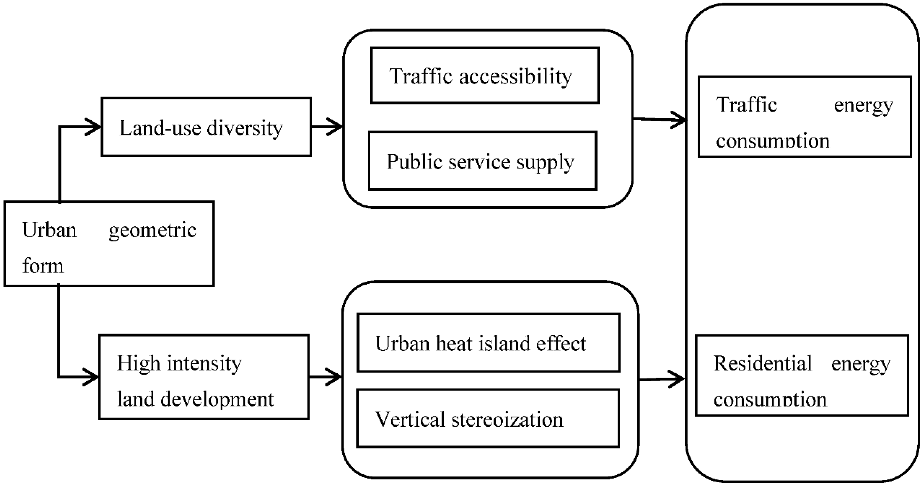
As mentioned above, compact urban form affects traffic and residential energy consumption through land use diversification and development intensity. According to the previous discussion, land diversification will make residents spend less time commuting. On the other hand, the less compact the urban boundary is, the longer the distance from the periphery to the centre will be, while the rent price decreases exponentially with the increase of the distance from the centre. Thus, families who reside in farther suburbs can afford much larger houses to meet their lifestyle needs [47]; however, the larger the area of affordable housing is, the higher the residential energy consumption is.
Therefore, the impact of the urban compact form on household energy consumption is uncertain which depends on the superposition effect of the two effects: if the urban compact form is dominated by reducing the impact of traffic on energy consumption, the urban compact form will reduce the energy consumption of residents; if the residential energy consumption is indirectly affected by the compensation of residential area, the higher the urban compact form, the higher the household energy consumption (Figure 1).
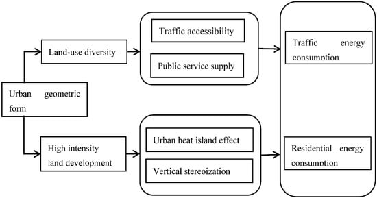
Figure 1.
Mechanism of Urban Geometric form on Household Energy Consumption.
If the urban compact form increases the residential energy consumption, it shows that the increase of household residential energy consumption due to the compensation of residential area by this spatial form is greater than the saving of transportation energy consumption due to the reduction of commuting distance. If the urban spatial form is originally very dense and the traffic congestion pressure will be great, then the compact form is more likely to cause congestion inside the city and increase the traffic energy consumption. We suspect that the negative effects of urban form will be more severe in cities with higher density. At the same time, if the urban transport infrastructure is improved, such as increasing the per capita road area, it may reduce congestion and reduce the commuting energy consumption without changing the original urban form and commuting distance, thus offsetting some of the negative impacts of compact form on residents‘ direct energy consumption.
3. Data and Empirical Strategy
3.1. Calculation of Household Energy Consumption
Overall, we have replicated Zhang et al.’s [48] methodology and expanded the estimation of household energy consumption to include the years 2000, 2010 and 2020. For individual cities, urban household energy consumption is measured as the sum of four sources: electricity (eec), gas (gec), transportation (tec) and central heating (cec). Specific formulas for calculating individual components of household energy consumption are reported in Table 1.

Table 1.
Estimation Methods of Urban Household Energy Consumption.
3.2. Qualifying Urban Geometric Form
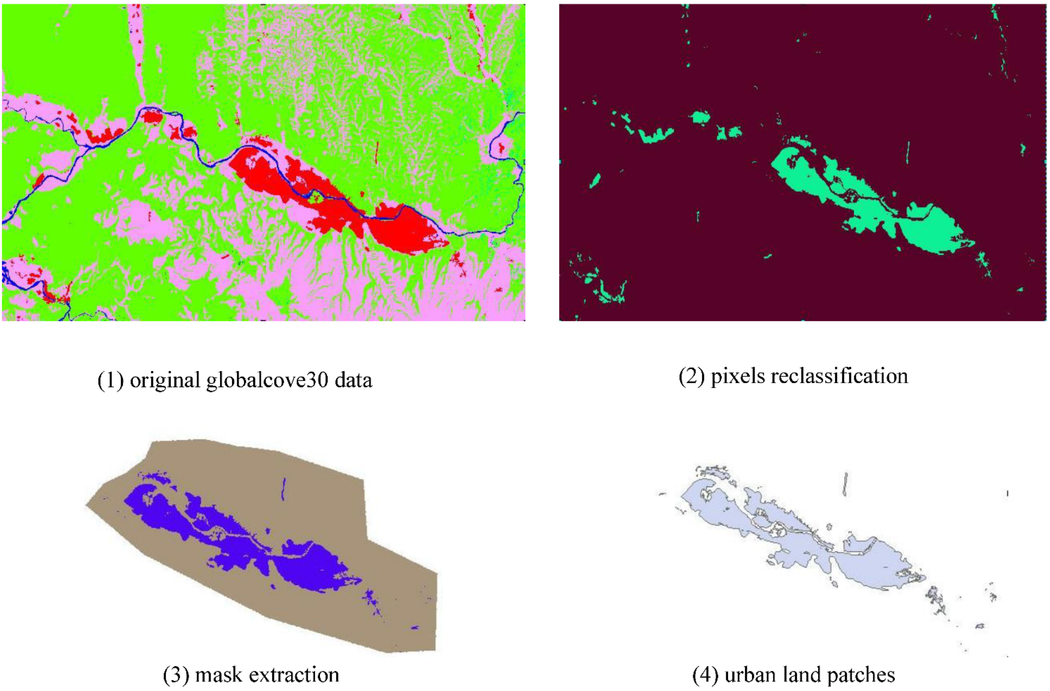
The urban geometric form data are extracted from the GlobalLand30 dataset released by the National Geomatics Center of China; this land cover data includes data for the years 2000, 2010 and 2020 with 30 m pixels. We use the impervious layer (code number 80) in the artificial cover type as the urban construction land.
The data processing steps are as follows: First, we reclassified the urban pixels. Since China’s urban sprawl is intervened by governmental land approvals and permissions, which implies that urban areas expand within urban jurisdictions. Thus, we delineate the contour boundary of the municipal district by boundary data of county-level administrative districts and a Google Earth historical map. Third, once the urban patches (contiguous or un-contiguous clusters of pixels) are identified, thus urban form index can be calculated. Figure 2 shows the data process taking Lanzhou city in 2010 as an example.

Figure 2.
Urban geometric form process.
The index of the moment of inertia (IMI) does not require continuity of urban form, which is more suitable to measure urban form with fragmentary, noncontiguous and polycentric characteristics. Thus, we use IMI to characterize the urban geometric form [14]. The arithmetic formula is given by:
In Formula (1), γi is the indicator which is equal to 1 when the cell i is the urban and 0 otherwise, r is the resolution of the raster and di is the distance of the cell I from the centroid. IMI is closer to 1 when the urban geometric form is heavily dispersed and closer to 1 when it is most compact for a given area.
3.3. Control Variables
Overall, we take urban density, urban structure, urbanization rate, urban population scale, urban household income, government intervention, energy-saving technology and infrastructure supply as control variables.
Firstly, urban density is measured by urban population density. Secondly, the urban monocentric or polycentric structures can be described as clustering of employment instead of the population at the district level [49]. We define the district with the highest density of employment as the main centre, and the polycentricity index is calculated as below:
where xit denotes the ratio between the employments of district i and the main centre in year t, n is the total number of districts for individual cities.
Besides these two variables, we also control other variables that may correlate with geometric and influence energy consumption. First, as mentioned above, urban household energy consumption has scale effects [30]. And the urban population is a proxy for urban size (pop). Second, richer families tend to travel much farther between the workplace and home, and we use average wages per worker as a proxy for household income (income). Third, energy supply needs infrastructure investments, which are funded by governments. Government fiscal expenditure covers infrastructure, urban planning and so on [50]. Thus, we better control governmental intervention and infrastructure supply in estimation and the public expenditure of municipal districts by the GDP of municipal districts is a proxy for governmental intervention (gov) and road density is a proxy for infrastructure supply (infra). Technological innovation can save household energy consumption, but it may also have a rebound effect [3]. We use the number of patents granted by prefecture-level cities to denote it (tech). Lastly, the urbanization rate is negatively correlated with household energy consumption [51,52], so we add the urbanization rate to control variables as well (urban).
3.4. Data Sources
The data on the electricity consumption of residents in each city is from China City Statistical Yearbook. The data on gas consumption, which consists of gas, coal gas, and natural gas, is gathered from China Urban Construction Statistical Yearbook. The data on central heating areas are gathered from China Urban Construction Statistical Yearbook, while unit coal consumption for heating is reported in Energy Conservation Design Standard in China. For transportation-related consumptions, the analysis accounts for taxis, buses and private vehicles. Following Zhang et al. [49], bus speed and fuel factors are set to 16 km/h and 32 L/100 km. Similarly, we set annual taxi mileage and the corresponding fuel factor to 12,000 km and 10 L/100 km. Statistics of private cars are mostly provincial total, and city-level data are only provided in China Regional Economic Statistical Yearbook for 2006–2013. For 2000 and 2020, we have responded in provincial and municipal yearbooks and statistical bulletins.
As control variables, the data on population density, urbanization rate, urban population scale and infrastructure supply comes from the corresponding annual China Urban Construction Statistical Yearbook. The data on household income and government intervention comes from the corresponding annual China Urban Statistical Yearbook. The data of patent authorization numbers of prefecture-level cities derive from the China Patent Announcement System on the official website of the State Intellectual Property Office. Statistical descriptions of variables are shown in Table 2.
Table 2.
Statistical description of variables.
According to the China Statistical Yearbook of 2021, per capita energy consumption is 0.438 tce (ton of standard coal equivalent). According to the proportion of energy consumption of urban and rural residents in China and the proportion of urbanization, we can estimate the urban household energy consumption is about 0.625 to 0.748 tce. In our study, the average urban household energy consumption is 0.672 tce, indicating that our estimation of urban household energy consumption is reliable.
3.5. Estimation Strategy
Since the core explanatory variable urban compact form is derived from high-definition land cover data in the years 2000, 2010 and 2020, we use panel data to explore the relationship between urban geometric form and household energy consumption. Panel data can reduce the heteroscedasticity problem that exists in cross-sectional data studies, thus more robust to identify the impact of urban form on urban household energy consumption. The empirical model is set as follows:
In Formula (3), hdeit denotes the urban household energy consumption of city i in period t, and compit denotes the geometric form of the city i. Xit is the set of control variables. ui denotes the city fixed effect and vt denotes the year fixed effect. εit is the residual term; this article focuses on the value of β0.
4. Results
4.1. Baseline Regression Results
Baseline regression results are shown in Table 3. Model 1 reported the estimation coefficients without control variables. Model 2 and 3 reported the impact of urban form compactness on household energy consumption. Early studies suggest that there is a U-shaped relationship between urban density and household energy consumption, so we put the first-order term and the quadratic term of urban density into the model to control, respectively.
Table 3.
Baseline regression results.
In these three models, the time fixed effect was added to control the macro impact, and the urban individual fixed effect was added to control the impact of urban individual differences. The results show that urban form compactness is negatively related to household energy consumption significantly. The setting of the first or second order of urban density does not affect the regression results. Besides, we conduct a VIF test for multicollinearity and cross-sectional dependence tests. VIF value of model 2 and model 3 is 1.96 and 2.84, which implies no covariance between the independent variables. As our sample data is short panel data, we use Pesaran’s CD test as the cross-sectional dependence test. The Pesaran’s CD test values of these three models are larger than 0.1, which implies no cross-sectional dependence.
The estimation coefficients of control variables in Table 3 meet our expectations. In model 2, both urban density and polycentric structure are significantly negatively correlated with household energy consumption, which echoes with the previous studies on the impact of urban form on household energy consumption [11,12,13,14,15,16,17,18,19,20,21,22,23,24,25,26,27]. For other control variables, urbanization rate and technology are positively correlated with household energy consumption. For every 1% increase in the urbanization rate, the household energy consumption will increase by 1.09%, and this result is consistent with previous studies by Wang [51,52]. As for saving-energy technology, for every 1% increase in the technology patents granted, the household energy consumption will increase by 1.04%, which implies that technological innovation has rebound effects [4,5]. Energy-saving technological innovations may improve energy efficiency, but residents may demand more comfortable lifestyles with more energy services in houses.
4.2. Endogeneity Problem
The benchmark model setting may have endogenous problems in three dimensions. Firstly, the reverse causal effect between key variables and dependent variables. Under the development goal of energy conservation and environmental protection, cities are more likely to use low-energy vehicles, such as subways. The construction of subways accelerates the urban land expansion, thereby increasing the perimeter of land patches and decreasing urban compactness; this reverse causality will make the estimation coefficient biased. Secondly, Sample selection bias. Sample data are not randomly generated, and the sample does not include Langfang, Tongliao, Jieyang, and other forty-four prefecture-level cities of the municipal districts due to data availability, which may cause estimation results biased. Lastly, the formation of urban geometric form is not a random process. Urban geometric form is influenced by urban planning and natural landscapes. Thus, it is difficult to use quasi-natural experiments to explore the causal relationship between urban geometric form and energy consumption.
Therefore, we use the instrumental variable method to solve the above endogenous bias. In this paper, the urban land ruggedness is the instrumental variable for urban geometric forms. As we mentioned above, urban geometric form is affected by natural topography and geomorphology. The land use of cities which are located in mountainous hills, valley terraces and coastal is scattered and winding, and their urban geometric index is lower; however, the cities located in the plain area tend to expand continuously due to weak topographic constraints, hence their urban geometric index is larger.
The regression results of instrumental variables are shown in Model 4 and Model 5 of Table 3. Model 4 does not add the quadratic term of urban density, while model 5 controls it. The results show that the LM statistics of the unidentifiable test and the F statistics of the weak instrumental variable test are large; it rejects the assumptions of unidentifiable and weak instrumental variable identification, indicating the instrumental variables selected in this paper are effective. The impact of urban compact form on household energy consumption is still significantly negative, which is similar to the previous benchmark regression results, and implies that the benchmark regression results may underestimate the reduction effect of urban compact form.
4.3. Robustness Checks
The above analysis of urban geometric form and household energy consumption may lead to some doubts. For example, urban central heating and summer cooling have obvious regional differences. Northern China is cold in winter, so central heating is needed, while the South needs cooling in hot summer. Although the above regression results have controlled the fixed effect of the city, the estimation results in this paper will be biased as long as the city suffered from a certain fluctuation in time (such as extreme weather).
To solve this problem, a series of robustness tests are conducted in this paper. Firstly, the heating energy consumption is deleted from the total household energy consumption, hence generating the index of hde_noheat. Secondly, time-varying climatic characteristics, such as temperature effects, are given further consideration. Suppose the average temperature in June of a year is higher than that of previous years. In that case, the increase of cooling energy consumption in summer is more likely due to the high temperature rather than the urban geometric form. Therefore, we use the annual average temperature in June to construct virtual variables (Year*Temp): suitable temperature area (15–25 degrees Celsius) and high-temperature area (higher than 25 degrees Celsius). And then add the cross-term of temperature suitable area, high-temperature area and year dummy variable to the regression equation.
In the above robustness tests (Table 4), we found that there is still a significant negative relationship between urban geometric form and household energy consumption, and the benchmark result is robust.
Table 4.
Robustness analysis.
4.4. Heterogeneity Analysis
China has a vast territory, and there are great differences in urban size, spatial location and urban planning process. Therefore, this paper further discusses the heterogeneity of urban geometric form and household energy consumption in the dimension of spatial structure, spatial location and urban scale. First, we divide cities into large cities (the population of municipal districts is more than 1 million), medium cities (500,000–1 million) and small cities (less than 500,000). Second, we divide cities into subgroups of Eastern China and Middle and West China. Lastly, the polycentric structure is grouped according to the mean value of the polycentricity index (0.274). If the value is smaller than the average value, then it belongs to the monocentric spatial structure subgroup; and if the value is larger than the average value, then it belongs to the polycentric spatial structure subgroup. The two-way fixed effect method is used to estimate these models.
The results in Table 5 show that the compact form of the larger-sized city group (Model 10) and medium city group (Model 11) significantly decreases the household energy consumption, and the compact form of the small city group (Model 12) does not significantly increase household energy consumptions; these results imply that the urban compact form has reduction effects only on large and medium-sized cities.
Table 5.
Heterogeneity analysis.
The spatial location heterogeneity analysis results are shown in model 13 and model 14; these results show that the impact of urban form on urban household energy consumption shows no spatial location heterogeneity, which implies the compact cities locate in the eastern, middle, or western parts of China have lower household energy consumption.
The analysis results of monocentric and polycentric structures are shown in Model 15 and Model 16. Previous studies suggest that polycentric spatial structure can effectively reduce urban energy consumption compared with monocentric structures [7,8,9,10]. We find that compact form has similar reduction effects both on the monocentric and polycentric spatial structures; these results imply that the previous studies on urban spatial structure may neglect the impact of urban geometric form, we may need to re-examine the robustness of the impact of the urban spatial structure on household energy consumption.
5. Mechanism Analysis
The impact of compact form on commuting time and per capita living area is analyzed to analyze the mechanism of urban geometric form on household energy consumption.
The commuting time data come from the China Time Use Survey (CTUS) of 2008, which is surveyed by the National Statistical Bureau in ten provinces, such as Beijing, Tianjin, Hebei, et al. CTUS takes the population aged 15–74 years old in the selected households as the survey object. The survey households consist of urban samples selected from the existing urban and rural household income and expenditure survey outlets in 10 provinces and cities. A total of 16,661 households and 37,142 persons are surveyed. CTUS adopts the internationally accepted time survey log form, and systematically records the various activities of all residents aged 15–74 in the surveyed households on rest days and working days (24 h) at intervals of every 10 min. We use the city code to match the respondents onto cities level, and then generate the commuting time data for work or school of each city. The cross-sectional data of 2010 are only used for this regression. The results are shown in Models 17–19 in Table 6.
Table 6.
Mechanism Analysis.
The regression coefficient of compact form in large and medium-sized cities is significantly negative, while that of small cities is significantly positive; this may be because the layout of public facilities in small cities is too concentrated, induced by large traffic at the same time confluence; it causes serious traffic congestion, and the energy consumption effect of transportation in the small city is reversed.
The living area per capita data comes from the ratio of the area of residential land to the total population of urban areas in the Statistical Yearbook of Urban Construction in China. As shown in Models 20–22 in Table 6, the coefficient of the compact form of medium-sized cities is significantly negative, indicating that the urban geometric form of large and small cities is not relevant to living area per capita. While the regression coefficient of the compact form of large cities is significantly positive (Model 20), indicating that the compact development of large cities improves the intensity of urban development. The land intensive development meets the needs of residents for better living conditions and larger residential areas, thereby improving the household energy consumption of residents in large cities.
Overall, compact form reduces household energy consumption in medium-sized cities by reducing commuting time and residential area and decreasing commuting time in large cities.
6. Conclusions and Discussion
We comprehensively analyze the impact of urban geometric form on household energy consumption with panel data of China’s 253 prefecture-level cities. Three main conclusions can be drawn:
- (1)
- The regression results of the overall sample show that the urban form will significantly reduce household energy consumption, and the estimation results are consistent by using the instrumental variables of land ruggedness. Robust checks take into account the central heating differences between the north and south, as well as extreme temperatures on household energy consumption, and find that the estimation results are robust.
- (2)
- The heterogeneity of urban geometric form and household energy consumption was analyzed in the dimension of spatial structure, spatial location, and urban scale; these results imply that the urban compact form has reduction effects only on large and medium-sized cities. We find that compact form has similar reduction effects both on the monocentric and polycentric spatial structures. What’s more, there is no spatial location heterogeneity, which implies the compact cities located in the eastern, middle, or western parts of China.
- (3)
- Mechanism analysis shows that urban geometric form reduces the household energy consumption in medium-sized cities by reducing commuting time and residential areas and decreasing commuting time in large cities. The land-intensive development meets the needs of residents for better living conditions and larger residential areas, thereby improving the household energy consumption of residents in large cities.
The findings in this study suggest that compact urban geometry is conducive to achieving carbon peaks and carbon neutrality goals; meanwhile, these approaches vary from urban size but not affected by region or location heterogeneity. Low-carbon urban planning policies should pay attention to urban size heterogeneity. Three policies can be drawn:
- (1)
- Decision-makers should pay attention to the full use of stock land and appropriately to promote the high-density development of urban land. Land infills, such as underutilized land and brownfields redevelopment, to reduce commute demands. In this process, the natural space should keep counteracting the negative effects of highly compact cities (i.e., urban heat island effect and lower quality of life).
- (2)
- As for large cities, decision-makers should pay attention to the rebound of residential energy consumption. Urban compact form increases the living area per capita in larger cities, which possibly increases residential energy consumption. Thus, it would be wise to increase the green building supply in large-sized cities. New built residential buildings should follow the green building standards, thereby effectively preventing the rebound of residential energy consumption.
- (3)
- As for small cities, the compact form of small cities cannot significantly reduce household energy consumption, which implies small cities should facilitate infrastructure supply to improve land utilization efficiency.
Although our study uses three years of panel data, the urban form high-definition data is only observed within two decades. Further studies may use observations with a larger time span, so much richer variations of urban land patches could be observed. Due to data availability, we have changed independent variables into commuting time and living area per capita in mechanism analysis. Further studies may use the moderation and mediation model to clearly articulate the mechanism of urban form on household energy consumption.
Author Contributions
Translation, software and data analysis, Y.G.; Conceptualization, resource preparation, data analysis, and writing—original draft, Y.H. All authors have read and agreed to the published version of the manuscript.
Funding
This work was funded by the Humanities and Social Sciences of Education Ministry of People’s Republic of China, grant number 17YJC790055.
Institutional Review Board Statement
Not applicable.
Informed Consent Statement
Not applicable.
Data Availability Statement
Not applicable.
Acknowledgments
We greatly appreciate Huang Qin of Harbin Institute of Technology (Shenzhen) for her thorough data processing.
Conflicts of Interest
The authors declare no conflict interest.
References
- Scotford, E.; Minas, S. Probing the hidden depths of climate law: Analysing national climate change legislation. Rev. Eur. Comp. Int. Environ. Law 2018, 28, 67–81. [Google Scholar] [CrossRef]
- Hepburn, C.; Qi, Y.; Stern, N.; Ward, B.; Xie, C.; Zenghelis, D. Towards carbon neutrality and China’s 14th Five-Year Plan: Clean energy transition, sustainable urban development, and investment priorities. Environ. Sci. Ecotechnol. 2021, 8, 100130. [Google Scholar] [CrossRef]
- Lin, B.; Liu, H. A study on the energy rebound effect of China’s residential building energy efficiency. Energy Build. 2015, 86, 608–618. [Google Scholar] [CrossRef]
- Zhang, J.; Chang, Y.; Zhang, L.; Li, D. Do technological innovations promote urban green development?—A spatial econometric analysis of 105 cities in China. J. Clean. Prod. 2018, 182, 395–403. [Google Scholar] [CrossRef]
- Fan, F.; Zhang, K.; Dai, S.; Wang, X. Decoupling analysis and rebound effect between China’s urban innovation capability and resource consumption. Technol. Anal. Strat. Manag. 2021, 5, 1–15. [Google Scholar] [CrossRef]
- Fan, J.-L.; Chen, K.-Y.; Zhang, X. Inequality of household energy and water consumption in China: An input-output analysis. J. Environ. Manag. 2020, 269, 110716. [Google Scholar] [CrossRef]
- Miao, L. Examining the impact factors of urban residential energy consumption and CO2 emissions in China—Evidence from city-level data. Ecol. Indic. 2017, 73, 29–37. [Google Scholar] [CrossRef]
- Bekun, F.V. Mitigating Emissions in India: Accounting for the Role of Real Income, Renewable Energy Consumption and Investment in Energy. Int. J. Energy Econ. Policy 2022, 12, 188–192. [Google Scholar] [CrossRef]
- de la Puente-Gil, Á.; González-Martínez, A.; Borge-Diez, D.; Blanes-Peiró, J.J.; De Simón-Martín, M. Electrical Consumption Profile Clusterization: Spanish Castilla y León Regional Health Services Building Stock as a Case Study. Environments 2018, 5, 133. [Google Scholar] [CrossRef]
- Pérez-Montalvo, E.; Zapata-Velásquez, M.-E.; Benítez-Vázquez, L.-M.; Cermeño-González, J.-M.; Alejandro-Miranda, J.; Martínez-Cabero, M.; de la Puente-Gil, Á. Model of monthly electricity consumption of healthcare buildings based on climatological variables using PCA and linear regression. Energy Rep. 2022, 8, 250–258. [Google Scholar] [CrossRef]
- Newman, P.W.G.; Kenworthy, J.R. Gasoline Consumption and Cities: A Comparison of U.S. Cities with a Global Survey. J. Am. Plan. Assoc. 1989, 55, 24–37. [Google Scholar] [CrossRef]
- Mindali, O.; Raveh, A.; Salomon, I. Urban density and energy consumption: A new look at old statistics. Transp. Res. Part A: Policy Pract. 2004, 38, 143–162. [Google Scholar] [CrossRef]
- Holden, E.; Norland, I.T. Three Challenges for the Compact City as a Sustainable Urban Form: Household Consumption of Energy and Transport in Eight Residential Areas in the Greater Oslo Region. Urban Stud. 2005, 42, 2145–2166. [Google Scholar] [CrossRef]
- Ewing, R.; Rong, F. The impact of urban form on U.S. residential energy use. Hous. Policy Debate 2008, 19, 1–30. [Google Scholar] [CrossRef]
- Liu, X.; Sweeney, J. Modelling the impact of urban form on household energy demand and related CO2 emissions in the Greater Dublin Region. Energy Policy 2012, 46, 359–369. [Google Scholar] [CrossRef]
- Kashem, S.B.; Irawan, A.; Wilson, B. Evaluating the dynamic impacts of urban form on transportation and environmental outcomes in US cities. Int. J. Environ. Sci. Technol. 2014, 11, 2233–2244. [Google Scholar] [CrossRef]
- Fang, C.; Wang, S.; Li, G. Changing urban forms and carbon dioxide emissions in China: A case study of 30 provincial capital cities. Appl. Energy 2015, 158, 519–531. [Google Scholar] [CrossRef]
- Lo, A.Y. Small is green? Urban form and sustainable consumption in selected OECD metropolitan areas. Land Use Policy 2016, 54, 212–220. [Google Scholar] [CrossRef]
- Lee, S.; Lee, B. The influence of urban form on GHG emissions in the U.S. household sector. Energy Policy 2014, 68, 534–549. [Google Scholar] [CrossRef]
- Zhu, K.; Tu, M.; Li, Y. Did Polycentric and Compact Structure Reduce Carbon Emissions? A Spatial Panel Data Analysis of 286 Chinese Cities from 2002 to 2019. Land 2022, 11, 185. [Google Scholar] [CrossRef]
- Kaza, N. Urban form and transportation energy consumption. Energy Policy 2019, 136, 111049. [Google Scholar] [CrossRef]
- Guo, R.; Leng, H.; Yuan, Q.; Song, S. Impact of Urban Form on CO2 Emissions under Different Socioeconomic Factors: Evidence from 132 Small and Medium-Sized Cities in China. Land 2022, 11, 713. [Google Scholar] [CrossRef]
- Liu, X.; Wang, M.; Qiang, W.; Wu, K.; Wang, X. Urban form, shrinking cities, and residential carbon emissions: Evidence from Chinese city-regions. Appl. Energy 2020, 261, 114409. [Google Scholar] [CrossRef]
- Buliung, R.N.; Kanaroglou, P.S. Urban Form and Household Activity-Travel Behavior. Growth Chang. 2006, 37, 172–199. [Google Scholar] [CrossRef]
- Brownstone, D.; Golob, T.F. The impact of residential density on vehicle usage and energy consumption. J. Urban Econ. 2009, 65, 91–98. [Google Scholar] [CrossRef]
- Liu, C.; Shen, Q. An empirical analysis of the influence of urban form on household travel and energy consumption. Comput. Environ. Urban Syst. 2011, 35, 347–357. [Google Scholar] [CrossRef]
- Debbage, N.; Shepherd, J.M. The urban heat island effect and city contiguity. Comput. Environ. Urban Syst. 2015, 54, 181–194. [Google Scholar] [CrossRef]
- Saiz, A. The Geographic Determinants of Housing Supply. Q. J. Econ. 2010, 125, 1253–1296. [Google Scholar] [CrossRef]
- Harari, M. Cities in Bad Shape: Urban Geometry in India. Am. Econ. Rev. 2020, 110, 2377–2421. [Google Scholar] [CrossRef]
- Liu, Y.; Fang, F.; Li, Y. Key issues of land use in China and implications for policy making. Land Use Policy 2014, 40, 6–12. [Google Scholar] [CrossRef]
- Lin, G.C.S.; Ho, S.P.S. The State, Land System, and Land Development Processes in Contemporary China. Ann. Assoc. Am. Geogr. 2005, 95, 411–436. [Google Scholar] [CrossRef]
- Liang, X.; Liu, X.; Li, X.; Chen, Y.; Tian, H.; Yao, Y. Delineating multi-scenario urban growth boundaries with a CA-based FLUS model and morphological method. Landsc. Urban Plan. 2018, 177, 47–63. [Google Scholar] [CrossRef]
- Jin, H.; Qian, Y.; Weingast, B.R. Regional decentralization and fiscal incentives: Federalism, Chinese style. J. Public Econ. 2005, 89, 1719–1742. [Google Scholar] [CrossRef]
- Lichtenberg, E.; Ding, C. Local officials as land developers: Urban spatial expansion in China. J. Urban Econ. 2009, 66, 57–64. [Google Scholar] [CrossRef]
- Wu, K.-Y.; Zhang, H. Land use dynamics, built-up land expansion patterns, and driving forces analysis of the fast-growing Hangzhou metropolitan area, eastern China (1978–2008). Appl. Geogr. 2012, 34, 137–145. [Google Scholar] [CrossRef]
- Feng, R.; Wang, K. The direct and lag effects of administrative division adjustment on urban expansion patterns in Chinese mega-urban agglomerations. Land Use Policy 2021, 112, 105805. [Google Scholar] [CrossRef]
- He, X. Energy effect of urban diversity: An empirical study from a land-use perspective. Energy Econ. 2022, 108, 105892. [Google Scholar] [CrossRef]
- Garrett, M.; Wachs, M. Transportation Planning on Trial: The Clean Air Act and Travel Forecasting; Sage Publications: Thousand Oaks, CA, USA, 1996; ISBN 978-0-8039-7352-7. [Google Scholar]
- Calthorpe, P. The Next American Metropolis: Ecology, Community, and the American Dream, 5th ed.; Princeton Architectural Press: New York, NY, USA, 1997; ISBN 978-1-878271-68-6. [Google Scholar]
- Larson, W.; Yezer, A. The energy implications of city size and density. J. Urban Econ. 2015, 90, 35–49. [Google Scholar] [CrossRef]
- Cervero, R.; Kockelman, K. Travel demand and the 3Ds: Density, diversity, and design. Transp. Res. Part D Transp. Environ. 1997, 2, 199–219. [Google Scholar] [CrossRef]
- Guerra, E.; Caudillo, C.; Goytia, C.; Quiros, T.P.; Rodriguez, C. Residential location, urban form, and household transportation spending in Greater Buenos Aires. J. Transp. Geogr. 2018, 72, 76–85. [Google Scholar] [CrossRef]
- Johnson, A. Bus Transit and Land Use: Illuminating the Interaction. J. Public Transp. 2003, 6, 21–39. [Google Scholar] [CrossRef]
- Glaeser, E.L.; Kahn, M.E. The greenness of cities: Carbon dioxide emissions and urban development. J. Urban Econ. 2010, 67, 404–418. [Google Scholar] [CrossRef]
- Larivière, I.; Lafrance, G. Modelling the electricity consumption of cities: Effect of urban density. Energy Econ. 1999, 21, 53–66. [Google Scholar] [CrossRef]
- Nichols, B.G.; Kockelman, K.M. Life-cycle energy implications of different residential settings: Recognizing buildings, travel, and public infrastructure. Energy Policy 2014, 68, 232–242. [Google Scholar] [CrossRef]
- Fujita, M.; Thisse, J.-F. Economics of Agglomeration: Cities, Industrial Location, and Regional Growth; Cambridge University Press: Cambridge, UK; New York, NY, USA, 2002; ISBN 978-0-521-80138-6. [Google Scholar]
- Zhang, Y.; Qin, Y.; Yan, W.; Zhang, J.; Zhang, L.; Lu, F.; Wang, X. Urban Types and Impact Factors on Carbon Emissions from Direct Energy Consumption of Residents in China. Geogr. Res. 2012, 32, 345–356. [Google Scholar]
- Zhang, T.; Sun, B.; Li, W. The economic performance of urban structure: From the perspective of Polycentricity and Monocentricity. Cities 2017, 68, 18–24. [Google Scholar] [CrossRef]
- Kwon, K. Polycentricity and the role of government-led development: Employment decentralization and concentration in the Seoul metropolitan area, 2000–2015. Cities 2021, 111, 103107. [Google Scholar] [CrossRef]
- Wang, M.; Madden, M.; Liu, X. Exploring the Relationship between Urban Forms and CO2 Emissions in 104 Chinese Cities. J. Urban Plan. Dev. 2017, 143, 04017014. [Google Scholar] [CrossRef]
- Wang, Q. Effects of urbanisation on energy consumption in China. Energy Policy 2014, 65, 332–339. [Google Scholar] [CrossRef]
Publisher’s Note: MDPI stays neutral with regard to jurisdictional claims in published maps and institutional affiliations. |
© 2022 by the authors. Licensee MDPI, Basel, Switzerland. This article is an open access article distributed under the terms and conditions of the Creative Commons Attribution (CC BY) license (https://creativecommons.org/licenses/by/4.0/).