Business Income Tax from Profit-Seeking Enterprises and Spatial Autocorrelation: Do Local Economic Characteristics Matter?

Abstract

We seek to explore whether local economic characteristics affect the collection of profit-seeking enterprise (PSE) income tax in Taiwan, by adopting panel data from 2001 to 2020 collected in its counties and cities. The results of this analysis of spatial econometric modeling indicate that the increase in sales of profit-seeking enterprises (SPSE) has a positive and significant direct effect on the collection of PSE income tax in this county and city. In terms of spatial spillover effects, when the number of profit-seeking enterprises (NPSE) in neighboring regions increases and the percentage of employees working in industrial sectors (PEI) increases, they will then impact the increase in PSE income tax collection in any particular county and city. We find that the amount of PSE income tax collection relates to the agglomeration economy. The findings of this study may be provided as a reference for local governments to conduct administrative construction on the formulation of PSE income tax collection.

1. Introduction

The level of business income tax reflects the strength of profitability of profit-seeking enterprises (hereafter PSE). The business income tax revenues from PSE in Taiwan grew from over TWD 100 billion 20 years ago to TWD 647.9 billion in 2019. The level of business income tax revenues dropped when the tax rate was reduced from 25% to 17% in 2010, in response to the 2008 global financial and 2009 European sovereign crises, while the total business income tax revenues exceeded TWD 400 billion in 2014 as the business environment improved; this figure rose further after the tax rate was adjusted to 20% in 2018. The percentage of business income tax revenues from PSE increased gradually from 10% of the total tax revenues, 20 years ago, to 24.4% in 2020; business income tax revenues have become the largest source of tax revenues in Taiwan. Aghion et al. [1] indicate that “taxation is central for many aspects of this environment: tax revenues fund public infrastructure, education and schools, legal systems, and much more.” Infrastructures are linked to the competitiveness ranking of most countries. According to the latest International Institute for Management Development (IMD), Taiwan’s ranking climbed from the 17th in 2018 to the 7th in 2022, the highest in the World Competitiveness Yearbook since 2013. Among the four indicators used to compile the rankings, Taiwan ranked 13th in terms of infrastructure. In addition to the international competitiveness ranking, the domestic competitiveness ranking among cities is also an important indicator of each citizen’s living satisfaction. This is the reason why local governments endeavor to create an environment conducive to business investments (e.g., expenditures related to economic development and the expenses for the city for agriculture, industry, transportation, and other economic services) with a variety of policies boosting the local economy. Evidence of the effects of local government’s duties and activities in regional developments, leading to spatial spillover in nearby regions, was identified in previous studies [2,3,4,5]. In the current study, we aim to investigate the growth of business income tax revenues from PSE in different cities from the perspective of spatial effects, due to local economic characteristics. This has existed in the literature but receives relatively little consideration.

The current study aims to fill the following three gaps. First, traditional econometrics suffer from limitations in terms of the analysis of spatial relations and values. This is because the assumptions of independent and identically distributed variables in traditional econometric methods are obviously not in line with the reality of spatial autocorrelation. As a result, model estimates and the inferences derived from them are not adequately robust [6]. Traditional approaches do not provide a full view of spatial effects and cannot truly reflect the influencing factors on business income tax revenues assessed by different regions. Geographic locations are relevant to business income tax revenues [7]. Studies report that ignorance of the spatial effects of regional economic developments causes bias [8]. As business income tax is the most important source of tax revenue in Taiwan, there may be a spatial autocorrelation between the amounts of PSE business income tax revenues among cities. However, few studies on this issue have investigated the possibility; therefore, we hope to fill this research gap in the existing studies.

Second, the spatial econometric results may allow us to verify whether local economic characteristics, such as infrastructure [1], expenditures on economic development [2], and employed population structures [9] exist within the overall agglomeration phenomenon for the spatial spillover effect on PSE income tax in neighboring regions. The spillover effects of local economic characteristics have been a focal point of extensive academic research. For example, Boarnet [4] states that the more robust the infrastructure in a region, the more attractive the production factors, such as capital and labor, from the neighboring areas. According to Cohen and Morrison Paul [5], public spending in a region, especially spending on infrastructure, creates positive spatial spillover effects on the economic growth of adjacent areas. López et al. [2] posit that the function of local governments is to provide a wide range of public services, which may lead to spatial spillover in nearby cities. Therefore, local governments’ fiscal policy and other administrative measures may have a direct or indirect influence on the endowment and flows of production factors. It also results in significant external effects on the business environment and naturally attracts PSE to establish a business presence and, in turn, contributing to the growth of business income tax revenues. As far as the spatial dependence of assessment of business income tax revenues is concerned, PSE behavior in geographic areas does not exist in silos. Rather, such phenomena are spatially related in some ways to adjacent areas. The distribution of business income tax revenues has a certain spatial pattern in which distribution intensity in different areas is subject to the influence of local environmental regulations and neighborhood effects. To our knowledge, no published studies in the field of taxation have identified the possible presence of local economic characteristic spillover effects on PSE income tax in neighboring regions.

Third, the World Health Organization (WHO) declared COVID-19 a public health emergency of international concern (PHEIC) on 30 January 2020 and then declared it a global pandemic on 11 March 2020 when it was shown to be highly infectious. The current COVID-19 pandemic has significantly changed people’s economic behaviors and has affected the development of many industries and countries, which inevitably impacted the collection of the PSEs’ income taxes. In the published literature, few studies have explored the effects of the COVID-19 pandemic on the income tax collection of such enterprises. The research period of this study covered the COVID-19 pandemic period, which exactly fills the gap in past studies.

The main purposes of this paper include: (1) exploring whether there is an overall agglomeration phenomenon for spatial autocorrelation in the net amount of PSE income tax in Taiwanese counties and cities, as well as the agglomeration situation in specific counties and cities; (2) exploring the direct effects of local economic characteristics on the collection of PSE income tax in local counties and cities; (3) exploring the spatial spillover effects of local economic characteristics in neighboring counties and cities on the collection of PSE income tax in local counties and cities. In the next chapters, we present a literature review and development of hypotheses, the empirical model, and the measurement of variables. The empirical analyses include spatial autocorrelation verification, a LISA cluster map, and spatial econometric modeling diagnosis, as well as the analysis of direct effects and spatial spillover effects. Lastly, we offer a conclusion and put forward policy implications, study limitations, and future study directions.

2. Literature Review and Development of Hypotheses

2.1. Spatial Econometric Models

According to Tobler’s [10] first law of geography (TFL), everything is related to everything else, but near things are more related than distant things. TFL is concerned with variable correlations in different spaces, i.e., spatial dependencies or spatial autocorrelation. Cliff and Ord [11] reported that the measurement of spatial autocorrelation is primarily focused on the values represented by neighboring spatial units (e.g., counties or states). Similar values indicate the existence of spatial autocorrelation. Goodchild [12] mentioned that spatial autocorrelation is the quantification of potential spatial dependency as a geographic phenomenon. It describes the degrees of similarity in the phenomenon at a location and the phenomenon at neighboring locations, to discriminate the status of spatial clustering. Spatial autocorrelation is the inspection of the spatial difference between variables in a given spatial unit and variables in nearby spaces. Anselin [13] regarded spatial autocorrelation as the potential spatial dependency of a geographic phenomenon. It is about describing the degree of spatial similarity between a specific region and nearby regions, to discern the characteristics of spatial clustering. Therefore, spatial autocorrelation is essentially a discussion of the correlation between a particular region and adjacent regions. It is an examination of the degree of nearby regional effects and an exploration of the potential influencing mechanism of spatial effects [14].

The analysis of spatial autocorrelation sheds light on whether the distribution of spatial phenomena is spatially autocorrelated. Spatial autocorrelation indicates a region’s greater similarity with neighboring regions or smaller similarity from distant (or not adjacent) regions. A high level of spatial autocorrelation in a region will cause spatial phenomena with the same characteristics to converge, while a low degree of spatial autocorrelation in a region will disperse the spatial phenomena through the space. Spatial autocorrelation comes in two extremes: (1) positive spatial autocorrelation, if the observed region is highly similar to neighboring regions and dissimilar to non-neighboring regions; and (2) negative spatial autocorrelation, if the observed region is dissimilar to nearby regions and similar to non-neighboring regions. Similarities in the economic conditions of nearby regions, the convergence of society and culture, and economic radiation in the form of population displacement, industrial development, and resource concentration all contribute to the increasing spatial clustering of adjacent regions. Contagion or diffusion effects, i.e., the so-called spatial spillover, may exist if an observed region is highly similar to neighboring regions; regional economic developments are subject to the influence of spatial factors. Hence, spatial spillover effects are an integral element of regional economic development.

Before 2000, a large amount of research based on spatial econometrics used cross-sectional data. As spatial econometrics developed, panel data modeling started to emerge after 2000 [15,16,17,18,19,20,21]. For instance, Schmidheiny [15] examined how income tax differences in the Basel metropolitan area affect the address selection strategy of residents. Karkalakos and Kotsogiannis [7] examined corporate income taxes in different provinces of Canada. They show that corporate income taxes in some provinces are affected by the tax policies of nearby provinces at the same time. Klemm and Van Parys [16] explored the influence of national business income tax rates in more than 40 countries in Latin America, the Caribbean, and Africa on foreign direct investments from 1985 to 2004. Loretz and Moore [17] studied the decision-making and planning of corporate taxes in 32 countries from 1998 to 2006. Kopczewska et al. [18] explored the influence of capital, labor, and consumption on public debt in 34 countries from 2002 to 2011. Cheng and Pu [19] reviewed the relationship between the effective rates of earned income taxes and capital income taxes and economic growth in 31 provinces in China from 2007 to 2013. Qi et al. [20] explored the influence of tax policies and taxation structures in 31 provinces in China from 2009 to 2018. Boly et al. [21] studied the spillover effect of national tax policies in Africa on foreign direct investments.

Spatial econometric models in the last ten years have been widely used in studies regarding land and real estate [22,23,24,25,26]. Liao and Wang [22] adopted a spatial quantile regression model to build a distance decay matrix, so as to control the effects of spatial dependence in Changsha, China, while Li et al. [25] adopted a spatial econometric method to distinguish the emotions of real estate investors and to analyze the correlation between the emotions of real estate investors and housing prices. Huang et al. [3] showed that an increase in tax income would have a positive direct effect on the local housing transaction volume, in turn, contributing to the growth of property tax. As mentioned above, business income tax revenues are the largest source of tax revenues in Taiwan, while few studies on the assessment of tax revenues in Taiwan refer to the perspective of the spatial effects of influencing factors on PSE income tax. Spatial statistics and spatial econometrics provide a new tool and method for the analysis and research of spatial data. Spatial econometric modeling can address those spatial effects that have a significant influence on economic activities and, hence, fill in the gap left by traditional econometric modeling.

2.2. Development of Hypotheses

This study involves the development of two major hypotheses: firstly, the direct influences of regional economic developments of the local cities/counties and the relevant employment and industry structures on the PSE income tax in the local cities/counties; secondly, the spatial spillover effect or spatial competition effect of regional economic developments in the neighboring cities/counties and the relevant employment and industry structures on PSE income tax in the neighboring cities/counties.

2.2.1. Regional Economic Characteristics and PSE Income Tax

The local economic characteristics of a certain region may change enterprise behaviors [27]. Good infrastructures in a certain region are beneficial to local development. The more sophisticated the infrastructures of a certain region, the more attractive the production factors, such as the capital and labor of neighboring regions [4]. Government expenditure is one of the major policy tools employed to achieve macroeconomic stability. Through fiscal expenditure, local governments could push forward economic development projects, creating an environment suitable for the survival and development of enterprises and, in turn, attracting more enterprises. The number of enterprises attracted by the local economy, as well as the profit-making capacities of such enterprises, would influence the levying of PSE income tax.

The spillover effect of the local economic environment has been investigated in many studies [2,4,5,28,29]. For instance, Cohen and Morrison Paul [5] and Pereira and Roca-Sagalés [29] discovered that public spending in a certain region, especially on infrastructure construction, has a positive spatial spillover effect on the economic growth of its neighboring regions. López et al. [2] suggested that the key function of local government is to provide comprehensive public services that will result in a spatial spillover effect in the neighboring cities. In addition, Kameda et al. [30] also mentioned that there is a very strong mutual interdependency between local economies when the border effect does not exist; that is, the government’s spending on the local economy could easily spill over to neighboring economies.

The local government’s fiscal policies and other administrative measures not only have direct or indirect influences on production factors, such as labor, capital, technology, information, and the flow of relevant factors but they also bring about important externality to the environmental regulation of business operations. These policies and measures naturally attract PSEs to establish business operation facilities, increasing the revenue of PSE income tax. Thus, hypothesis 1a (direct effect) and hypothesis 1b (spatial spillover effect) are proposed as follows:

Hypothesis 1 (1a).

The regional economic characteristics of the local cities/counties (expenditure of economic development, the number of PSE, and the sales amount of PSEs) have significant influences on the net revenues of PSE income tax in local cities/counties.

Hypothesis 1 (1b).

The regional economic characteristics of the neighboring cities/counties (expenditure of economic development, the number of PSE, and the sales amount of PSE) have significant influences on the net revenues of PSE income tax in the neighboring cities/counties.

2.2.2. Employed Population Structure, Industrial Structure, and PSE Income Tax

The continuous adjustment of the industrial structure could promote a country’s economic and social development. In particular, there is a close relationship between industrial structure and economic growth [31,32,33]. Bashir et al. [33] pointed out that there was bidirectional causality between the added values of industries and the variables of economic growth in Indonesia’s economy. Conversely, Zhao and Tang [34] probed the relationship between the industrial structure and economic growth of China and Russia from 1995 to 2008. Relatively speaking, compared to the Russian economy, the Chinese economy focused more on the manufacturing industry and less on the service industry. China’s economic growth in 2003–2008 was faster than in 1996–2002. The main reason for such rapid growth in 2003–2008 was primarily attributed to contributions from the manufacturing industry and, to a lesser extent, the service industry. Regarding the aspect of human resources, Fan et al. [35] mentioned that there was an obvious positive correlation between economic growth and the proportion of technicians employed in the state-owned sector, which was labor-intensive, or in the capital-intensive mixed sector. Zhao and Tang [34] pointed out that in Russia, the service industry contributed most strongly to economic growth, followed by the primary industry, driven by the mining, petroleum, and natural gas extraction industries. Kraftova et al. [31] studied the influence of industrial structure on the economic growth dynamics of the Czech Republic. They suggested that if the Czech Republic increased the contribution of the second industry to the total added value, the labor productivity of the whole national economy would be promoted. However, if the contribution of the third industry to the total added value were increased, the labor productivity of the whole national economy would decline.

These transitions in the industrial structure might increase productivity and promote economic growth, continually speeding up the structure’s changes and transformations. Such a process might influence the enterprise income tax. Adjusting the whole industrial structure needs support and assistance from the government’s tax revenue. This means that there is a correlation, to some extent, between the industrial structure and the government’s tax revenue. Past studies suggested that the allocation of production factors could influence the evolution of the industrial structure, affecting economic growth and taxation. Labor is one of the most important production factors [9]. The allocation of labor in the industrial structure could be deemed a disposition of the said structure. Hence, hypothesis 2a (direct effect) and hypothesis 2b (spatial spillover effect) are proposed as follows:

Hypothesis 2 (2a).

The employed population structure and the industrial structure of the local Taiwan cities/counties (proportion of industrial workers; the proportion of workers in the service industry; the proportion of workers in the 25–44 age group; the proportion of workers in the 45–64 age group) have a significant influence on the net revenues of PSE income tax in local cities/counties.

Hypothesis 2 (2b).

The employed population structure and the industrial structure of the neighboring cities/counties (proportion of industrial workers; the proportion of workers in the service industry; the proportion of workers in the 25–44 age group; the proportion of workers in the 45–64 age group) have a significant influence on the net revenues of PSE income tax in the neighboring cities/counties.

The following section explains the research methodology and the empirical model of this paper.

3. Materials and Methods

Setting of Spatial Econometric Model

LeSage and Pace [6] developed the spatial Durbin model (SDM) by including the lags of dependent variables and the lags of independent variables to derive better estimates. Based on SDM, we constructed an empirical model as follows:

$$\ln NABI{T}_{it}=\rho {{\displaystyle \sum }}_{j=1}^N{W}_{ij}\ln NABI{T}_{jt}+\alpha +\mathsf{\beta }{\mathbf{X}}^{\prime }+\mathsf{\theta }\mathbf{W}{\mathbf{X}}^{\prime }+{\mu }_i+{\epsilon }_{it}, i\ne j$$

(1)

where $\rho$ is the spatial lag coefficient, the spatial autocorrelation coefficient of the dependent variable for neighboring regions to indicate the direction and degree of influence of $\ln NABI{T}_{jt}$ in the nearby region on $\ln NABI{T}_{it}$ in this region. The test on the spatial lag coefficient $\rho$ further examines the spatial relationships between neighboring areas. A statistically significant $\rho$ shows the spatial dependency between the dependent variable of neighboring regions and the dependent variable of this specific region. $\rho \ne 0$ indicates the existence of spatial relationships with neighboring regions. A $\rho$ greater than 0 indicates positive spatial autocorrelation. $\ln NABI{T}_{it}$ is the dependent variable; i, j are local cities in Taiwan; $\mathbf{W}=W_{ij}$ is the spatial weights matrix, which consists of a square matrix that is symmetrical from left to right and from top to bottom, with the number of rows and columns indicating the number of regions. The contiguity matrix is employed to define neighboring relationships, with 1 indicating two nearby regions and 0 if they are not. The diagonal line also indicates zero to indicate that there is no neighboring relationship between one city and the particular region in question. $\mathbf{W}$ is typically defined to express the spatial neighboring relationships of the n positions:

$$\mathbf{W}=W_{ij}=\left[\begin{array}{cccc}{w}_{11}& w_{12}& \dots & w_{1n}\\ w_{21}& w_{22}& \dots & w_{2n}\\ ⋮& ⋮& \dots & ⋮\\ w_{n1}& w_{n2}& \dots & w_{nn}\end{array}\right]$$

(2)

The spatial neighboring of units is classified into rook contiguity, bishop contiguity, or queen contiguity. Rook contiguity refers to a common edge between two spatial units, while bishop contiguity is the sharing of a common vertex, and queen contiguity is the sharing of a common edge or a common vertex [36]. In this study, we employed queen contiguity to define spatial neighboring relationships. A number of rules are available for the construction of spatial weight matrices. Those most frequently used are based on neighboring relationships and distance. $\mathbf{W}$ expresses the spatial and neighboring relationships of 22 cities. The three island counties do not demonstrate neighboring relationships with each other; hence, the value is zero.

$NABI{T}_{it}$ is the net and actually assessed business income tax from PSE of city i in year t. Business income taxes are levied from the net incomes of PSE. The tax filing period runs from 1 May to 31 May annually. If the headquarters of PSE are in Taiwan, income from outside Taiwan should be consolidated and assessed for business income tax. The calculation of taxable income is based on subtracting all costs and expenses from total revenue during the year. $W_{ij}\ln NABI{T}_{jt}$ is the spatial autocorrelation matrix of the dependent variable of nearby regions and is an endogenous variable, indicating the influence of $\ln NABI{T}_{jt}$ in neighboring regions j on $\ln NABI{T}_{it}$ in region i. $\alpha$ is the constant term, and $\mathsf{\beta }$ is the coefficient vector. X = [$P{D}_{it},\ln EE{D}_{it}$, $\ln NPS{E}_{it}$, $\ln SPS{E}_{it},PE{I}_{it}$, $PE{S}_{it}$, $PE{Y}_{it}$, $PE{M}_{it}$] is the vector of independent variables. $\mathsf{\beta }{\mathbf{X}}^{\prime }$ is the original effect of each independent variable in this region on $\ln NABI{T}_{it}$. $\mathsf{\theta }$ is the spatial autocorrelation coefficient vector of the independent variable of neighboring regions, reflecting the influence of our independent variable vector X, in nearby regions on $\ln NABI{T}_{it}$ in this region. $\mathsf{\theta }\mathbf{W}{\mathbf{X}}^{\prime }$ is the spatial autocorrelation matrix of the independent variables of nearby regions, reflecting the spatial effects of all independent variables of the neighboring areas. A positive $\theta$ value suggests proactive effects from neighboring regions on $\ln NABI{T}_{it}$, while a negative $\theta$ value indicates competitive effects from nearby regions on this region. ${\mu }_i$ represents the spatial effects of city i. Error terms, ${\epsilon }_{it}$, are independently distributed for spatial autocorrelation. In this study, the variables and definitions are organized as defined in

Table 1. Variables and definitions.

Variable	Definition
$NABI{T}_{it}$	$NABI{T}_{it}$ is the net and actually assessed business income tax from PSE of city i in year t. Business income taxes are levied from the net incomes of PSE.
$P{D}_{it}$	$P{D}_{it}$ is the number of people on average per square kilometer of city i in year t, is calculated by dividing the number of people with household registration by the area of the land.
$EE{D}_{it}$	$EE{D}_{it}$ represents expenditures related to the economic development of city i in year t, is the expenses for the city for agriculture, industry, transportation, and other economic services.
$NPS{E}_{it}$	$NPS{E}_{it}$ is the number of companies in city i in year t with tax registration per Article 28 of Chapter 5 of the Value-added and Non-value-added Business Tax Act.
$SPS{E}_{it}$	$SPS{E}_{it}$ is the sales of PSE in city i at year t according to tax filings or assessments.
$PE{I}_{it}$	$PE{I}_{it}$ is the percentage of employees working in industrial sectors in city i in year t, is the number of employees in the industrial sectors (including mining and quarrying; manufacturing; utilities; construction) as a percentage of the total workforce (number of employees in industrial sectors/total number of employees).
$PE{S}_{it}$	$PE{S}_{it}$ is the percentage of employees working in service sectors in city i in year t, is to the number of employees in the service sectors (including wholesale and retail; hotels and restaurants; transportation, warehousing and communication; finance and insurance; real estate; professional, scientific, technical and education services; health and social work activities; cultural, sport and recreational services; public administration) as a percentage of the total workforce (number of employees in service sectors/total employees).
$PE{Y}_{it}$	$PE{Y}_{it}$ is the number of employees aged between 25 and 44/total employees in city i at year t.
$PE{M}_{it}$	$PE{M}_{it}$ is the number of employees aged between 45 and 64/total employees in city i at year t.

.

Considering the issue of inflation, we deflate the nominal values with the consumer price index (CPI) into real values to eliminate the influence of inflation. The nominal $NABI{T}_{it}$, $EE{D}_{it}$, and $SPS{E}_{it}$ are deflated to eliminate such an influence. For example, the nominal NABIT from PSE/CPI × 100 = real value of NABIT from PSE. To reduce the variance of the variables, we take a natural logarithm of the above five variables. In this study, Stata 16.0 was utilized to analyze the spatial econometric model.

4. Results

4.1. Summary Statistics

We collected our data from 2001 to 2020 for 22 cities in Taiwan from the R.O.C. (Taiwan) National Statistics website (https://eng.stat.gov.tw/mp.asp?mp=5, accessed on 20 May 2021).

Table 2. Summary of the descriptive statistics.

Var.	Obs.	Mean	Std. Dev.	Min	25th Perc.	Med	75th Perc.	Max
NABIT	440	16,579,062.6	32,770,355.7	6874.4	743,511.9	2,402,589.0	18,700,000.0	218,651,080.7
PD	440	1498.1	2165.1	61.2	304.3	752.1	1644.4	9951.5
EED	440	6588.6	6915.1	670.7	2303.7	3804.9	7138.7	36,884.3
NPSE	440	54,335.7	61,332.0	748.4	16,041.5	23,044.8	77,629.4	244,591.5
SPSE	440	1,548,995,474.7	2,534,559,957.5	1,650,626.6	162,000,000.0	399,000,000.0	2,070,000,000.0	14,085,753,950.0
PEI	440	32.9	9.8	14.6	25.0	31.8	41.2	52.8
PES	440	59.1	11.4	38.4	50.1	57.0	69.5	81.6
PEY	440	54.4	5.0	37.5	51.5	55.0	57.7	64.0
PEM	440	35.0	5.5	22.4	31.1	35.1	38.5	54.0

Note: For the definition of variables, please refer to Section 3: Methodology.

and

Table 3. Pearson correlation analysis.

	NABIT	PD	EED	NPSE	SPSE	PEI	PES	PEY	PEM
NABIT	1
PD	0.783 ***	1
EED	0.713 ***	0.410 ***	1
NPSE	0.775 ***	0.477 ***	0.886 ***	1
SPSE	0.963 ***	0.760 ***	0.770 ***	0.857 ***	1
PEI	−0.056	−0.192 ***	0.089	0.173 ***	−0.008	1
PES	0.297 ***	0.488 ***	0.108 *	0.110 *	0.262 ***	−0.745 ***	1
PEY	0.124 **	0.233 ***	0.056	0.200 ***	0.166 ***	0.389 ***	−0.111 *	1
PEM	0.042	−0.034	0.049	−0.080	−0.006	−0.463 ***	0.376 ***	−0.907 ***	1

Note: * p < 0.05; ** p < 0.01; *** p < 0.001.

summarize the descriptive statistics and the correlation matrix with raw values for variables, respectively. Table 2 shows a drastic difference between the maximum and minimum values of NABIT, the dependent variable, and the independent variables related to regional economic features, such as EED, NPSE, and SPSE. This finding indicates the imbalance in Taiwan’s regional economic development.

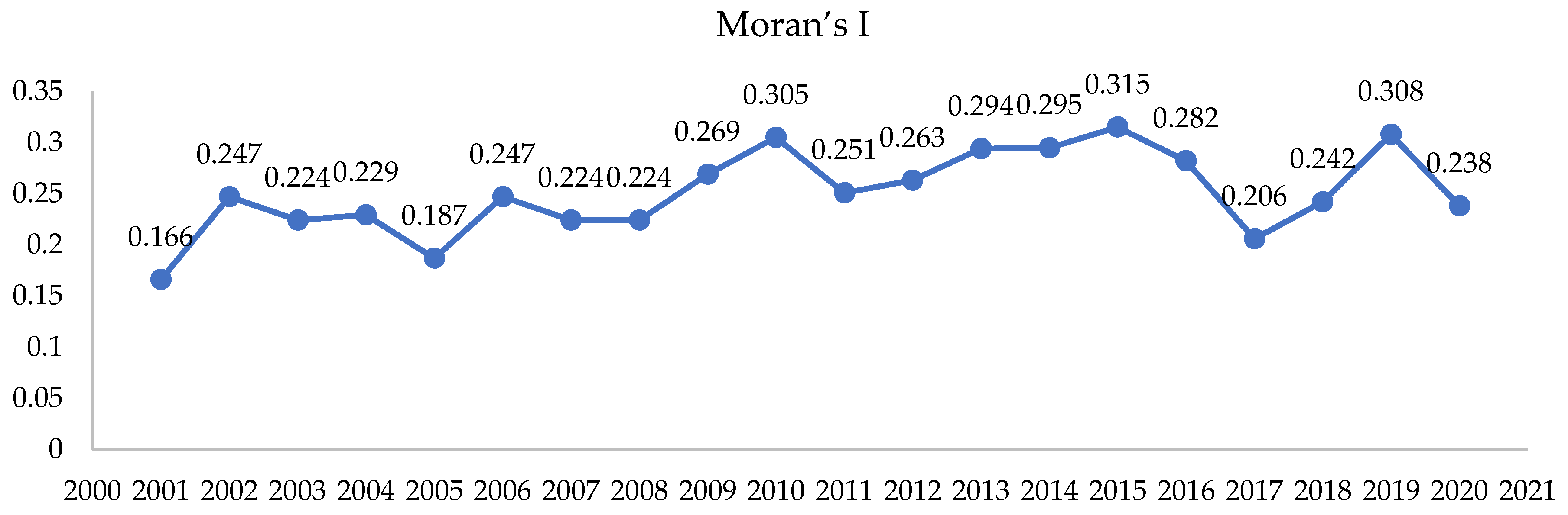
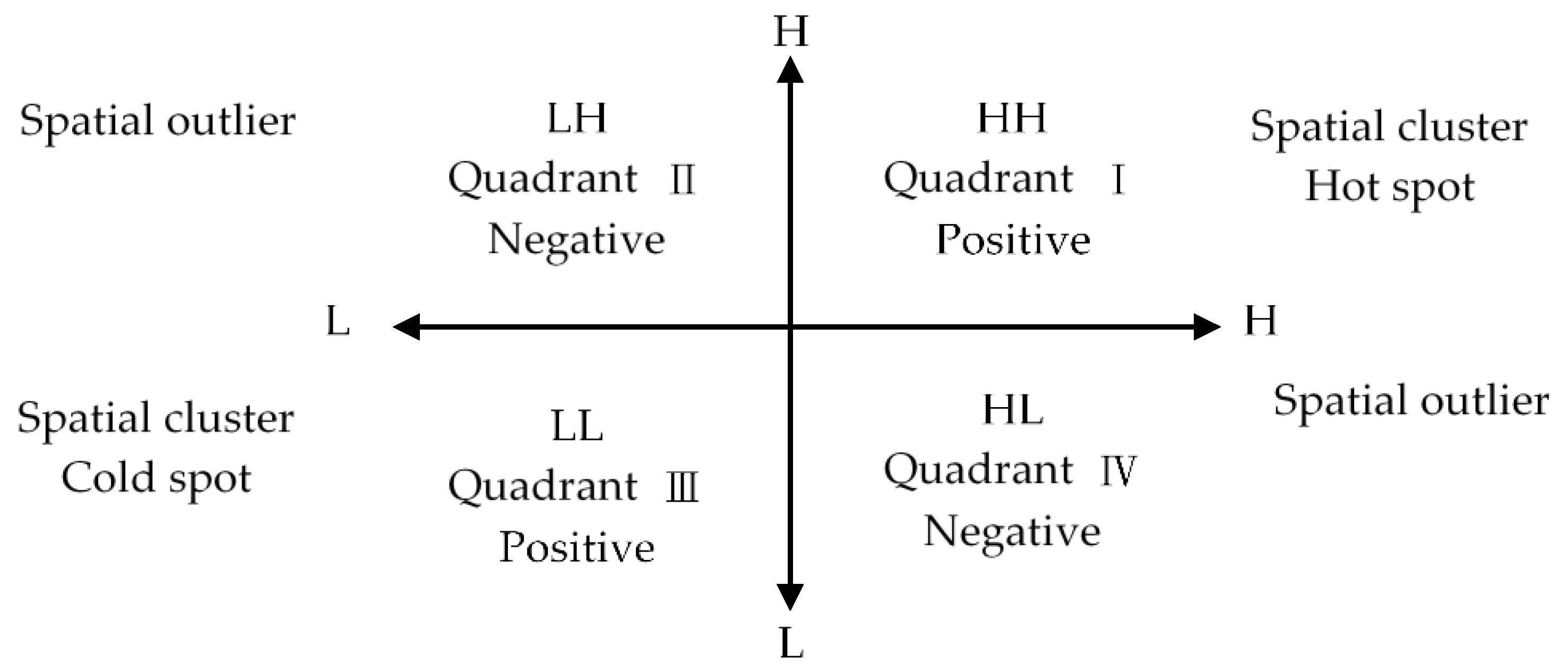
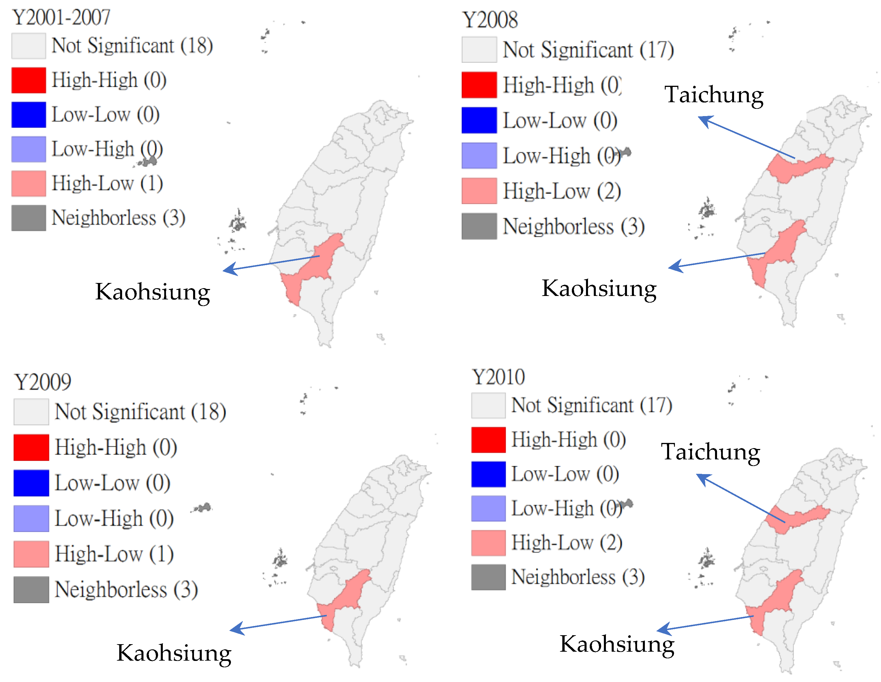
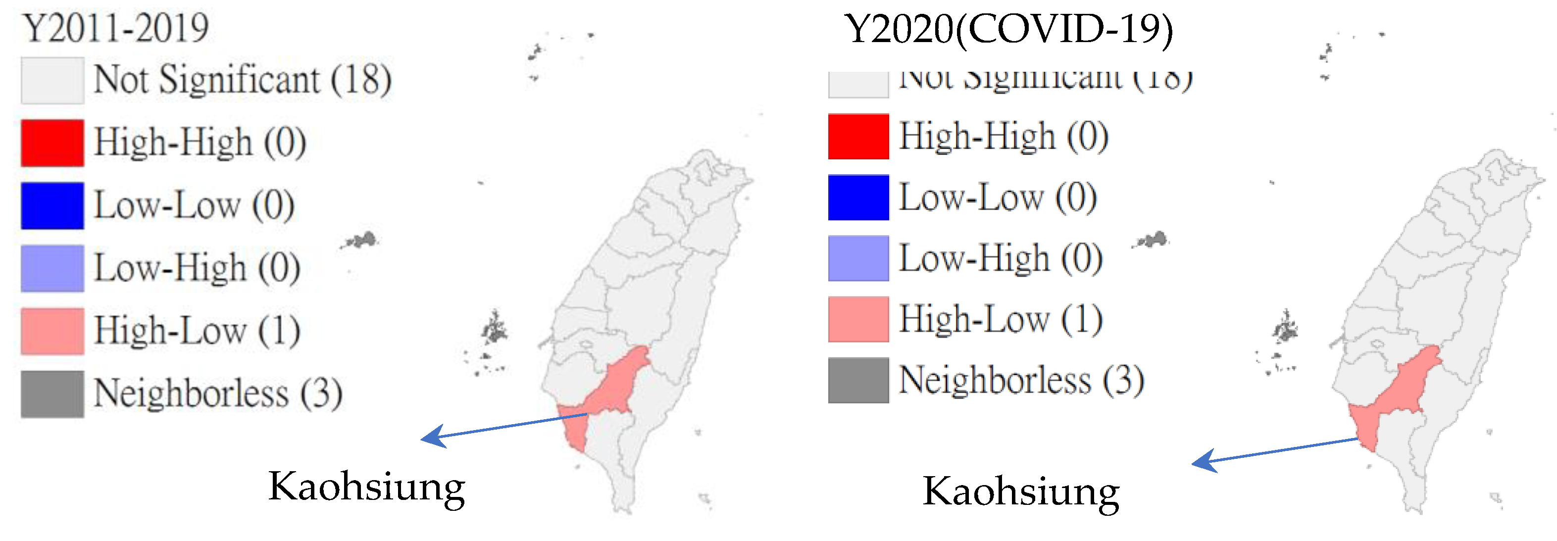
4.2. Spatial Autocorrelation Tests

Among the spatial autocorrelation measurements, Moran’s I boasts better statistical power and is the most widely used spatial autocorrelation indicator. The range of Moran’s I values is in [−1, 1]. A value closer to 1 indicates a stronger positive spatial autocorrelation, while a value closer to −1 presents a stronger negative spatial autocorrelation [37]. The technique establishes an understanding of spatial clusters but cannot analyze regional changes or pinpoint the spatial distribution of hot spots.

All Moran’s I values are at a 5% significance level, suggesting a significant and positive spatial autocorrelation in NABIT from PSE among cities, indicating strong spatial clustering in PSE’s NABIT among various cities in Taiwan. Figure 1 presents the trend of Moran’s I-values for the NABIT from PSE among cities from 2001 to 2020; the values gradually trend upward.

Anselin [38] divides the local indicator of spatial association (LISA) statistics into four quadrants according to the degree of spatial clustering, to indicate the spatial relationships between this region and the neighboring regions. LISA provides an explanatory model of spatial interactions. Moran’s I is unable to reveal spatial clustering among cities or the spatial autocorrelation of different regions, and LISA can address this gap.

Among the four quadrants of LISA (Figure 2), the first and the third quadrants are the areas where similar values cluster. The first quadrant shows a high degree of clustering, while the third quadrant shows a low degree of clustering. The first and third quadrants represent the pull-through effect, i.e., the influence caused by changes in the nearby regions. This is usually referred to as the basis of spatial diffusion. Significant and positive spatial autocorrelation refers to a given region being surrounded by regions of similar attribute values. This is known as spatial clustering. A spatial cluster can be classified as either a hot spot or a cold spot. The first quadrant indicates hot spots (denoted as High-High), in which the observed values are high for both the researched region and the adjacent regions. The third quadrant indicates cold spots (Low-Low), in which the observed values are low for both the researched region and the adjacent regions.

The second and fourth quadrants are indicators of negative spatial autocorrelation and are the areas where different values cluster. These quadrants show mutual exclusion effects, i.e., a negative influence of the changes in adjacent regions on the observed values. The second quadrant, Low-High, is where low observed values are surrounded by high values, while the fourth quadrant, High-Low, is where high observed values are surrounded by low values. Significantly negative spatial autocorrelation suggests great variance between the observed values in this region and the observed values in neighboring regions. This is called a spatial outlier.

The test results of the LISA analysis are graphed into a map and segmented with the levels of significance. Different colored blocks indicate the degree of spatial autocorrelation. This facilitates the observation of changes in the LISA analysis, clustered at different time points, and visualizes the changes in spatial structures over time.

Figure 3 shows the LISA clustering of the PSE’s NABIT in Taiwan, indicating that the statistics are significant for Kaohsiung from 2001 to 2020 and in Taichung in 2008 and 2010. The LISA results for other cities are not significant. The LISA values for NABIT from PSE in Kaohsiung and Taichung are classified as High-Low, suggesting that PSE’s NABIT in Kaohsiung and Taichung are higher than the overall mean and that those from nearby cities are lower than the overall mean. The differences are statistically significant.

4.3. Panel Unit-Root Test

When the unit root exists in the time sequence, the data generation process is of a random-walk nature; that is, these variables have non-stationary time sequence features. The expected values of the variable or variance of the non-stationary time sequence are not fixed. Consequently, the estimated results of these models do not apply to the prediction. This study suggests that it is necessary to carry out the unit root test of NABIT on the dependent variable. Our dependent variable includes time-series data; hence, unit-root tests are required. The panel unit-root test methods used by this paper are tests of the Levin-Lin-Chu unit-root [39] and the Harris-Tzavalis unit-root [40].

Table 4. Unit root test.

Unit Root Test	Stat.	p-Value
Levin-Lin-Chu unit-root test H0: Panels contain unit roots
Unadjusted t	−6.104
Adjusted t*	−2.310	0.014
Harris-Tzavalis unit-root test H0: Panels contain unit roots
Rho	0.793	0.022

’s panel unit-root test results report no unit roots for the stationary time series data of NABIT, using PSE as the dependent variable. Hence, there is no need to proceed with the first difference.

4.4. Spatial Model Selection

LeSage and Pace [6] reported that SDM can be simplified into either the SAR model or SEM. Consequently, tests are conducted on the hypotheses for model selection. Given that H₀: $\theta$ = 0, if the null hypothesis is rejected, SDM cannot be simplified into the SAR model; hence, SDM is a more reasonable option. Given that H₀: $\theta$ + $\rho \mathsf{\beta }=0$, if the null hypothesis is rejected, SDM cannot be simplified into SEM; therefore, SDM is a more reasonable option.

As shown in

Table 5. The results of spatial autoregressive model (SAR).

$Y_{it}=\alpha +\rho {\displaystyle \sum }_{j=1}^N{W}_{ij}{Y}_{jt}+\mathsf{\beta }{X}_{it}+{\mu }_i+{\epsilon }_{it}$, ${\epsilon }_{it}~N\left(0,{\sigma }^2\right),i\ne j$ $\mathrm{where}{Y}_{it}\mathrm{is}\mathrm{the}\mathrm{dependent}\mathrm{variable};\rho \mathrm{is}\mathrm{the}\mathrm{spatial}\mathrm{autocorrelation}\mathrm{coefficient};W_{ij}\mathrm{is}\mathrm{the}\mathrm{spatial}\mathrm{weight}\mathrm{matrix};\mathsf{\beta }\mathrm{is}\mathrm{the}\mathrm{coefficient};X_{it}$$\mathrm{is}\mathrm{the}\mathrm{independent}\mathrm{variable};{\mu }_i$$\mathrm{is}\mathrm{the}\mathrm{spatial}\mathrm{effect};{\epsilon }_{it}$ is the error term.
Var.	Model 1 SAR with spatial fixed effects		Model 2 SAR with spatial and time fixed effects		Model 3 SAR with random effects
	Coef.	Std. Err.	Coef.	Std. Err.	Coef.	Std. Err.
PD	0.001 **	0.000	0.001 *	0.000	0.000	0.000
lnEED	0.047	0.044	0.016	0.044	0.031	0.050
lnNPSE	0.383 *	0.187	−0.122	0.239	0.163	0.149
lnSPSE	0.986 ***	0.119	0.917 ***	0.131	0.930 ***	0.114
PEI	0.018	0.015	−0.002	0.015	0.026 **	0.010
PES	0.011	0.013	0.006	0.013	0.019 *	0.009
PEY	0.014	0.013	0.099 ***	0.016	0.029 *	0.014
PEM	−0.027 *	0.013	0.040	0.022	0.034 *	0.013
Constant					−10.968 ***	1.301
n		440		440		440
$\mathrm{Spatial}\rho$	0.399 ***	0.041	0.096	0.059	0.045 *	0.022
within R2	0.644		0.338		0.603
between R2	0.743		0.843		0.983
overall R2	0.713		0.812		0.963
Log-likelihood	−80.155		−41.872		−166.972
Wald test	$H_0: \theta =0$ $x^2$ = 64.30 *** p-value = 0.000		$H_0: \theta =0$ $x^2$ = 74.17 *** p-value = 0.000		$H_0: \theta =0$ $x^2$ = 117.24 *** p-value = 0.000
Likelihood-ratio test	$\mathrm{LR}{x}^2$ = 60.85 *** p-value = 0.000		$\mathrm{LR}{x}^2$ = 74.03 *** p-value = 0.000		$\mathrm{LR}{x}^2$ = 110.33 *** p-value = 0.000

Note: * p < 0.05, ** p < 0.01, *** p < 0.001. Only equations with significant coefficients (p < 0.05) are added to illustrate every empirical result. Model 1: $\ln NABI{T}_{it}=0.001{\ast \mathrm{PD}}_{it}+0.383{\ast \mathrm{lnNPSE}}_{it}+0.986{\ast \mathrm{lnSPSE}}_{it}-0.027{\ast \mathrm{PME}}_{it}$; Model 2: $\ln NABI{T}_{it}=0.001{\ast \mathrm{PD}}_{it}+0.917{\ast \mathrm{lnSPSE}}_{it}+0.099{\ast \mathrm{PMY}}_{it}$; Model 3:$\ln NABI{T}_{it}=-10.968+0.93{\ast \mathrm{lnSPSE}}_{it}+0.026{\ast \mathrm{PEI}}_{it}+0.019{\ast \mathrm{PES}}_{it}+0.029{\ast \mathrm{PEY}}_{it}+0.034{\ast \mathrm{PEM}}_{it}.$

, between an SAR model with spatial fixed effects and an SDM with spatial fixed effects, Wald’s $x^2$ = 64.30 (p < 0.001) and the likelihood ratio’s $x^2$ = 60.85 (p < 0.001) show that an SDM with spatial fixed effects is a more reasonable option. According to

Table 6. The results of spatial error model (SEM).

$Y_{it}=\alpha +\mathsf{\beta }{X}_{it}+{\mu }_i+{\phi }_{it}$ $\mathrm{where}{Y}_{it}\mathrm{is}\mathrm{the}\mathrm{dependent}\mathrm{variable};\mathrm{the}\mathrm{subscript}i\mathrm{is}\mathrm{the}\mathrm{region};\mathsf{\beta }\mathrm{is}\mathrm{the}\mathrm{regression}\mathrm{coefficient};X_{it}$$\mathrm{is}\mathrm{the}\mathrm{independent}\mathrm{variable};{\mu }_{i }$$\mathrm{is}\mathrm{the}\mathrm{spatial}\mathrm{effect};{\phi }_{it}$ is the error term. ${\phi }_{it}=\lambda {\displaystyle \sum }_{j=1}^N{W}_{ij}{\phi }_{jt}+{\epsilon }_{it},{\epsilon }_{it}~N\left(0,{\sigma }^2\right),i\ne j$ $\mathrm{where}\lambda \mathrm{is}\mathrm{the}\mathrm{spatial}\mathrm{autocorrelation}\mathrm{coefficient}\mathrm{of}\mathrm{the}\mathrm{error}\mathrm{term};W_{ij}$$\mathrm{is}\mathrm{the}\mathrm{spatial}\mathrm{weight}\mathrm{matrix};{\epsilon }_{it}$ is the error term of spatial autocorrelation.
Var.	Model 4 SEM with spatial fixed effects		Model 5 SEM with spatial and time fixed effects		Model 6 SEM with random effects
	Coef.	Std. Err.	Coef.	Std. Err.	Coef.	Std. Err.
PD	0.001 **	0.000	0.001 *	0.000	0.000	0.000
lnEED	0.036	0.042	0.009	0.042	0.061	0.044
lnNPSE	0.295	0.192	−0.087	0.231	−0.033	0.106
lnSPSE	1.036 ***	0.120	0.942 ***	0.127	1.095 ***	0.078
PEI	0.012	0.015	0.000	0.015	0.012	0.008
PES	0.007	0.013	0.005	0.013	0.003	0.007
PEY	0.047 **	0.015	0.095 ***	0.015	0.049 **	0.015
PEM	0.014	0.016	0.041 *	0.021	0.030 *	0.015
Constant					−11.400 ***	1.412
n		440		440		440
$\mathrm{Spatial}\lambda$	0.513 ***	0.057	0.064	0.065	0.479 ***	0.053
within R2	0.593		0.340		0.584
between R2	0.840		0.796		0.990
overall R2	0.819		0.770		0.966
Log-likelihood	−88.290		−40.610		−138.804
Wald test	$H_0:\theta +\rho \mathsf{\beta }=0$ $x^2$ = 67.76 *** p-value = 0.000		$H_0:\theta +\rho \mathsf{\beta }=0$ $x^2$ = 78.60 *** p-value = 0.000		$H_0:\theta +\rho \mathsf{\beta }=0$ $x^2$ = 120.94 *** p-value = 0.000
Likelihood-ratio test	$\mathrm{LR}{x}^2$ = 77.12 *** p-value = 0.000		$\mathrm{LR}{x}^2$ = 71.51 *** p-value = 0.000		$\mathrm{LR}{x}^2$ = 54.00 *** p-value = 0.000

Note: * p < 0.05, ** p < 0.01, *** p < 0.001. Only equations with significant coefficients (p < 0.05) are added to illustrate every empirical result. Model 4:$\ln NABI{T}_{it}=0.001{\ast \mathrm{PD}}_{it}+1.036{\ast \mathrm{lnSPSE}}_{it}+0.047{\ast \mathrm{PEY}}_{it}$; Model 5: $\ln NABI{T}_{it}=0.001{\ast \mathrm{PD}}_{it}+0.942{\ast \mathrm{lnSPSE}}_{it}+0.095{\ast \mathrm{PEY}}_{it}$; Model 6:$\ln NABI{T}_{it}=-11.40+1.095{\ast \mathrm{lnSPSE}}_{it}+0.049{\ast \mathrm{PEY}}_{it}+0.030{\ast \mathrm{PEM}}_{it}$.

, between SEM with spatial fixed effects and SDM with spatial fixed effects, Wald’s $x^2$ = 67.76 (p < 0.001) and the likelihood-ratio test of $x^2$ = 77.12 (p < 0.001) indicate that an SDM with spatial fixed effects is a more reasonable option. The results of the Wald and likelihood-ratio tests on the three models (SAR, SEM, and SDM) suggest that SDM is a more reasonable option.

4.5. SDMs Results

For the overall model goodness-of-fit (GoF), the estimates of the spatial models are based on the maximum likelihood estimation (MLE). The non-linear test values of MLE are derived from the model and the coefficients are maximized. Only the GoF tests based on non-linear principles, such as the log-likelihood, the Akaike information criterion (AIC), and the Schwartz Bayesian information criterion (BIC) can be used. The largest log-likelihood value or the smallest AIC or BIC value indicate the better model. The AIC and BIC values refer to the assessment of model GoF, in which a smaller value indicates greater GoF.

However, the spatially lagged coefficient $\rho$ of Model 8 did not reach a significant level ($\rho$ = 0.035, p > 0.05). Models 7 and 9 of

Table 7. The results of spatial Durbin model (SDM).

$Y_{it}=\alpha +\mathsf{\beta }{X}_{it}+{\mu }_i+{\phi }_{it}$ $\mathrm{where}{Y}_{it}\mathrm{is}\mathrm{the}\mathrm{dependent}\mathrm{variable};\mathrm{the}\mathrm{subscript}i\mathrm{is}\mathrm{the}\mathrm{region};\mathsf{\beta }$$\mathrm{is}\mathrm{the}\mathrm{regression}\mathrm{coefficient};X_{it}$$\mathrm{is}\mathrm{the}\mathrm{independent}\mathrm{variable};{\mu }_{i }$$\mathrm{is}\mathrm{the}\mathrm{spatial}\mathrm{effect};{\phi }_{it}$ is the error term. ${\phi }_{it}=\lambda {\displaystyle \sum }_{j=1}^N{W}_{ij}{\phi }_{jt}+{\epsilon }_{it}, {\epsilon }_{it}~N\left(0,{\sigma }^2\right)$$,i\ne j$ $\mathrm{where}\lambda \mathrm{is}\mathrm{the}\mathrm{spatial}\mathrm{autocorrelation}\mathrm{coefficient}\mathrm{of}\mathrm{the}\mathrm{error}\mathrm{term};W_{ij}$$\mathrm{is}\mathrm{the}\mathrm{spatial}\mathrm{weight}\mathrm{matrix};{\epsilon }_{it}$ is the error term of spatial autocorrelation.
Var.	Model 7 SDM with spatial fixed effects		Model 8 SDM with spatial and time fixed effects		Model 9 SDM with random effects
	Coef.	Std. Err.	Coef.	Std. Err.	Coef.	Std. Err.
PD	0.001 *	0.000	0.000	0.000	0.000	0.000
lnEED	0.024	0.042	0.033	0.040	0.034	0.043
lnNPSE	0.171	0.189	0.510 *	0.237	0.019	0.121
lnSPSE	0.866 ***	0.120	1.067 ***	0.125	1.027 ***	0.091
PEI	0.021	0.015	0.018	0.015	0.017	0.011
PES	0.003	0.013	−0.004	0.013	0.002	0.010
PEY	0.017	0.016	0.016	0.017	0.030 *	0.015
PEM	−0.029	0.018	−0.004	0.021	−0.014	0.016
W × PD	−0.001 *	0.000	−0.001 *	0.000	0.000	0.000
W × lnEED	−0.078	0.062	0.002	0.062	−0.021	0.064
W × lnNPSE	1.865 ***	0.465	2.065 ***	0.555	0.457	0.257
W × lnSPSE	−0.310	0.221	0.246	0.254	−0.444 *	0.173
W ×PEI	0.038	0.021	0.020	0.021	0.032 *	0.015
W × PES	0.032	0.021	0.007	0.021	0.030 *	0.015
W × PEY	−0.023	0.026	−0.011	0.030	−0.062 **	0.019
W × PEM	−0.029	0.026	−0.012	0.035	−0.010	0.023
Constant					−7.664 ***	1.551
n		440		440		440
$\mathrm{Spatial}\rho$	0.328 ***	0.055	0.035	0.075	0.340 ***	0.050
within R2	0.704		0.672		0.675
between R2	0.646		0.672		0.981
overall R2	0.621		0.651		0.964
Log-likelihood	−49.728		−4.855		−111.805
AIC	135.457		45.710		263.611
BIC	209.019		119.272		345.346
$\mathrm{Hausman}{x}^2$	18.62 *		15.29
Hausman p-value	0.0170		0.0537

Note: * p < 0.05, ** p < 0.01, *** p < 0.001. Only equations with significant coefficients (p < 0.05) are added to illustrate every empirical result. Model 7:$\ln NABI{T}_{it}=0.001{\ast \mathrm{PD}}_{it}+0.866{\ast \mathrm{lnSPSE}}_{it}-0.001\ast \mathrm{W}\times PD+1.865\ast \mathrm{W}\times {\mathrm{lnNPSE}}_{it}$; Model 8:$\ln NABI{T}_{it}=0.510{\ast \mathrm{lnNPSE}}_{it}+1.067{\ast \mathrm{lnSPSE}}_{it}-0.001\ast \mathrm{W}\times PD+2.065\ast \mathrm{W}\times {\mathrm{lnNPSE}}_{it}$; Model 9:$\ln NABI{T}_{it}=-7.664+1.027{\ast \mathrm{lnSPSE}}_{it}+0.03{\ast \mathrm{PEY}}_{it}-0.444\ast \mathrm{W}\times {\mathrm{lnSPSE}}_{it}+0.032\ast \mathrm{W}\times {\mathrm{PEI}}_{it}+0.03\ast \mathrm{W}\times {\mathrm{PES}}_{it}-0.062\ast \mathrm{W}\times {\mathrm{PEY}}_{it}$.

show that the Hausman test is $x^2$ = 18.62, p < 0.05, thereby rejecting the random effect hypothesis, indicating that Model 7 is better than Model 9 in this study. The log-likelihood value of Model 7 is larger than that of Model 9. The AIC and BIC values in Model 7 are smaller than those of Model 9. Therefore, we use Model 7 to examine the spatial fixed-effect SDM. The spatial lag coefficient $\rho$ of SDM with the spatial fixed effects is significantly positive ($\rho$ = 0.328, p < 0.001), showing spatial autocorrelation with PSE’s NABIT in different cities, and justifies the inclusion of spatial effects in our study. The results from the SDM with spatial fixed effects are the same as those presented from global Moran’s I and exhibit a positive spatial autocorrelation, overall. Previously, we have learned about the agglomeration situation in specific counties and cities by means of LISA analysis. For example, Taichung and Kaohsiung belong to H-L districts with a high PSE income tax in their own counties and cities and a low PSE income tax in their neighboring counties and cities. LISA results are aimed at specific counties and cities, which are not contradictory to the results of SDM and global Moran’s I being aimed at the whole country.

4.6. SDM, Direct, and Spillover and Spatial Fixed Effects

SDM also takes into account the spatial interaction effects [8]. The direct reference of results on spatially estimated parameters to determine whether the existence of spatial spillover leads to inaccurate conclusions due to feedback effects. As the model includes spatially lagged independent variables and dependent variables, the estimates cannot directly reflect marginal effects or the direct influence of independent variables on dependent variables. We decomposed SDM into direct, spatial spillover, and total effects.

Table 8. Direct, indirect, and total effects of SDM with spatial fixed effects.

Variables	Direct Effect		Indirect Effect		Total Effect
	Coef.	Std. Err.	Coef.	Std. Err.	Coef.	Std. Err.
PD	0.001	0.000	−0.001	0.001	0.000	0.001
lnEED	0.017	0.042	−0.082	0.077	−0.066	0.097
lnNPSE	0.341	0.199	2.290 ***	0.563	2.631 ***	0.678
lnSPSE	0.858 ***	0.116	−0.017	0.270	0.841 **	0.314
PEI	0.025	0.015	0.054 *	0.024	0.079 *	0.032
PES	0.006	0.014	0.041	0.026	0.047	0.033
PEY	0.016	0.016	−0.023	0.030	−0.007	0.031
PEM	−0.032	0.018	−0.049	0.030	−0.081 **	0.030

Note: * p < 0.05, ** p < 0.01, *** p < 0.001.

demonstrates the results of the decomposition of SDM with spatial fixed effects. The increase in sales of profit-seeking enterprises (SPSE) has a positive and significant impact on the collection of PSE income tax in this region. If the sales of PSE increase by 1 percentage point in this region, then the actual net amount of PSE income tax will increase by 0.858 percentage points.

This study has found two factors with positive and significant spatial spillover effects: the number of profit-seeking enterprises (NPSE) and the percentage of employees working in industrial sectors (PEI). When NPSE in neighboring regions increased by 1 percentage point, the PSE income tax in this region fell by 2.29 percentage points. When the PEI in neighboring regions increased by 1 percentage point, the PSE income tax in this region rose by 0.054 percentage points. Due to the influence of the agglomeration factor, local economic environment characteristics correlate with business behaviors [41]. The two factors have obviously proved that the amount of PSE income tax relates to the agglomeration economy.

Finally, in terms of the total effect, the increases in NPSE, SPSE, and PEI are all beneficial to the collection of PSE income tax. However, the increase in PEM runs adverse to the collection of PSE income tax.

5. Conclusions and Implications

5.1. Conclusions

Based on the spatial correlation and spatial dependency described by Moran’s I and the LISA analyses, the NABITs from PSE in Taiwan cities are spatially clustered. Compared to other cities, the PSE’s NABITs in Kaohsiung and Taichung are more spatially clustered and exhibit a negative spatial autocorrelation. The difference between these two municipalities and nearby cities is significant. This is particularly the case with Kaohsiung from 2001 to 2020, compared to adjacent cities. The difference between Taichung and adjacent cities is only significant in 2008 and 2010. The first export zone in the world was set up in Kaohsiung. As an industrial zone established by Taiwan to attract foreign capital, it has made significant contributions to the economic development of Taiwan. Many PSE, especially small-and-medium enterprises in the field of manufacturing, have been subsequently set up and concentrated in Kaohsiung. Over time, Kaohsiung has become a city of industrial clusters. In Taichung, the Central Taiwan Science Park started to attract companies in 2006 and encouraged manufacturers in the surrounding areas to upgrade and transform. As a result, Taichung has become a technology hub in central Taiwan. Development in central Taiwan is centered on Taichung, while development in southern Taiwan is centered on Kaohsiung.

We have found that the increase in the sales of profit-seeking enterprises (SPSE) has a positive and significant direct effect on the PSE income tax in this region. The increases in the number of profit-seeking enterprises (NPSE) and the percentage of employees working in industrial sectors (PEI) have positive and significant spatial spillover effects on PSE income tax in neighboring counties and cities (NPSE-PEI spillover effect). The occurrence of this phenomenon may be related to Taiwan’s tax system and transport infrastructure. Payment of PSE income tax is exempted for those enterprises with an annual taxable income of no more than TWD 120,000, while a 20% tax is levied on the total taxable income of a PSE with an annual taxable income of more than TWD 120,000. According to the statistics of the Ministry of Finance, half of the Taiwanese enterprises have a tax amount of zero. These are likely to be the cooperation manufacturers of large companies. Tax-paying companies are generally registered in six special municipalities, but living and operating business cost in the municipalities is significantly higher than in their nearby regions [26]; therefore, small businesses and workforces may choose to locate and live in non-metropolitan areas. Taiwan’s tax system and transport infrastructure may explain the NPSE-PEI spillover effect on PSE income tax in neighboring counties and cities.

Moreover, we seem to find that the amount of PSE income tax relates to the agglomeration economy. Csíki et al. [41] mentioned that the location factor affecting the site selection of a company is most closely related to the development of infrastructure. The agglomeration of a company is a dynamic process. Along with continuous economic development in various counties and cities, the spatial agglomeration of economic activities and industrial distribution has led to the continuous development of many companies, with six special municipalities as the core. Therefore, better infrastructure construction in the region, stronger industrial development strength, and land development conducive to building factories are the three factors that will effectively attract more PSEs to set up factories and operate in these areas. All these factors have a positive impact on the increase in PSE income tax.

5.2. Policy Implications

López et al. [2] have indicated that the effects of a specific local government’s investment in public services can lead to spatial spillover in nearby cities, result in external effects on the business environment, and attract PSE to establish a business presence. This, in turn, increases the local government’s PSE income tax revenues. Lu et al. [42] found that when central and local governments cooperate to open prestigious universities and foster land development in the underdeveloped areas of populous cities, this accelerates local economic development and population growth. Hwang and Quigley [43] mentioned that the growth of income taxes from PSEs reflects the results of the business cycle and may influence the land developers’ decision-making process in housing markets. In other words, growth in NABIT should be counted as the result of successful urban planning.

As the economies of the various Taiwan cities/counties develop, the agglomeration of PSEs has become a dynamic process. Many industries have gradually gathered around the six special municipalities, due to the spatial agglomeration effect of economic activities and the distribution of different industries. In Taiwan, cities/counties with a higher population density always have greater budget resources, tending to be more economically developed. Hence, PSEs often gather in cities/counties with highly concentrated populations. Studying the influential factors of the net revenues of PSE income tax is an indispensable process for acquiring a deeper understanding of the economic developments of the various cities/counties in Taiwan. As far as the practical conditions are concerned, regional differences exist between the industrial structures and economic development levels of the various cities/counties, resulting in an imbalance in Taiwan’s economic development, thereby hindering economic growth. The empirical findings of this study can contribute to our understanding of the spatial autocorrelation of the net revenues of the PSE income tax in various cities/counties. In addition, this data can also be used as a reference for government administration. It is expected that the findings of this study will prove beneficial to the comprehensive economic development of Taiwan and the amelioration of rural-urban disparity.

5.3. Research Limitations

Given the limitations regarding the procurement of research materials, this study only probes into the spatial autocorrelation of the net revenues of PSE income tax in the various Taiwanese cities/counties and the relevant factors. The spatial effects should include spatial autocorrelation and heterogeneity. Regional heterogeneity implies a lack of autocorrelation between different regions, such as downtown areas and suburbs, developed and underdeveloped regions, and others. For instance, the economic developments of the special municipalities and non-special municipalities of Taiwan differ quite profoundly from each other. When spatial heterogeneity and autocorrelation coexist, the traditional methods of econometrics would no longer be applicable. However, this may become a complex condition that poses some difficulty in terms of distinguishing between spatial heterogeneity and autocorrelation. This problem could probably be solved only by acquiring more suitable research materials and utilizing more sophisticated spatial econometric models.

5.4. Future Research Directions

Due to spatial autocorrelation or heterogeneity among different cities/counties, the influences of the regional economic features, the employed population, and the industrial structure on the levying of PSE income tax in each city/county are different. This study explores the economic conditions of the various cities/counties through the analytical method of spatial econometric models, which provide a better understanding of the determining factors of the levying amount of PSE income tax. Meanwhile, it is also believed that other variables are worth investigating. Therefore, it is suggested that subsequent researchers look for suitable variables for modeling and analysis through the relevant literature or other theories. For instance, the influence of the development of the real estate market on the levying of income tax may be further studied in the future. Another suggestion to subsequent researchers is to extend this topic to the discussion of spatial heterogeneity and utilize more sophisticated spatial econometric models to discover more conclusions.

References

1. Aghion, P.; Akcigit, U.; Cagé, J.; Kerr, W.R. Taxation, corruption, and growth. Eur. Econ. Rev. 2016, 86, 24–51. [Google Scholar] [CrossRef]
2. López, F.A.; Martinez-Ortiz, P.J.; Cegarra-Navarro, J.G. Spatial spillovers in public expenditure on a municipal level in Spain. Ann. Reg. Sci. 2017, 58, 39–65. [Google Scholar] [CrossRef]
3. Huang, H.C.; Chu, S.H.; Peng, C.L.; Liao, T.H. The spatial spillover effect of local fiscal expenditure in regional housing market: The case of Taiwan. J. Hous. Built Environ. 2022, 37, 1339–1365. [Google Scholar] [CrossRef]
4. Boarnet, M. Spillovers and the locational effects of public infrastructure. J. Reg. Sci. 1998, 38, 381–400. [Google Scholar] [CrossRef]
5. Cohen, J.P.; Paul, C.J.M. Public Infrastructure Investment, Interstate Spatial Spillovers, and Manufacturing Costs. Rev. Econ. Stat. 2004, 86, 551–560. Available online: https://www.jstor.org/stable/3211646 (accessed on 22 October 2021). [CrossRef]
6. LeSage, J.; Pace, R.K. Introduction to Spatial Econometrics; CRC Press, Taylor & Francis Group: New York, NY, USA, 2009. [Google Scholar] [CrossRef]
7. Karkalakos, S.; Kotsogiannis, C. A Spatial Analysis of Provincial Corporate Income Tax Responses: Evidence from Canada. Can. J. Econ. 2007, 40, 782–811. Available online: http://www.jstor.org/stable/4620632 (accessed on 22 October 2021). [CrossRef]
8. Rey, S.J.; Montouri, B.D. US regional income convergence: A spatial econometric perspective. Reg. Stud. 1999, 33, 143–156. [Google Scholar] [CrossRef]
9. Cissé, I.; Dubé, J.; Brunelle, C. New business location: How local characteristics influence individual location decision? Ann. Reg. Sci. 2020, 64, 185–214. [Google Scholar] [CrossRef]
10. Tobler, W.R. A computer movie simulating urban growth in the Detroit region. Econ. Geogr. 1970, 46, 234–240. [Google Scholar] [CrossRef]
11. Cliff, A.D.; Ord, J.K. Spatial Autocorrelation; Pion: London, UK, 1973. [Google Scholar]
12. Goodchild, M.F. A spatial analytical perspective on geographic information system. Int. J. Geogr. Inf. Syst. 1987, 1, 327–334. [Google Scholar] [CrossRef]
13. Anselin, L. Spatial Econometrics: Methods and Models; Kluwer Academic: Dordrecht, The Netherlands, 1988. [Google Scholar] [CrossRef]
14. Goodchild, M.F.; Anselin, L.; Appelbaum, R.P.; Harthorn, B.H. Toward spatially integrated social science. Int. Reg. Sci. Rev. 2000, 23, 139–159. [Google Scholar] [CrossRef]
15. Schmidheiny, K. Income segregation and local progressive taxation: Empirical evidence from Switzerland. J. Public Econ. 2006, 90, 429–458. [Google Scholar] [CrossRef]
16. Klemm, A.; Van Parys, S. Empirical evidence on the effects of tax incentives. Int. Tax Public Financ. 2012, 19, 393–423. [Google Scholar] [CrossRef]
17. Loretz, S.; Moore, P.J. Corporate tax competition between firms. Int. Inst. Public Financ. 2013, 20, 725–752. [Google Scholar] [CrossRef]
18. Kopczewska, K.; Kudła, J.; Walczyk, K.; Kruszewski, R.; Kocia, A. Spillover effects of taxes on government debt: A spatial panel approach. Policy Stud. 2016, 37, 274–293. [Google Scholar] [CrossRef]
19. Cheng, X.; Pu, Y.P. Effective Tax Rates, Spatial Spillover, and Economic Growth in China: An Empirical Study Based on the Spatial Durbin Model. Ann. Econ. Financ. 2017, 18, 73–97. Available online: http://aeconf.com/Articles/May2017/aef180104.pdf (accessed on 10 July 2022).
20. Qi, Y.; Peng, W.; Xiong, N.N. The effects of fiscal and tax incentives on regional innovation capability: Text extraction based on python. Mathematics 2020, 8, 1193. [Google Scholar] [CrossRef]
21. Boly, A.; Coulibaly, S.; Kéré, E. Tax policy, foreign direct investment and spillover effects in Africa. J. Afr. Econ. 2020, 29, 306–331. [Google Scholar] [CrossRef]
22. Liao, W.C.; Wang, X. Hedonic house prices and spatial quantile regression. J. Hous. Econ. 2012, 21, 16–27. [Google Scholar] [CrossRef]
23. Tu, Y.; Sun, H.; Yu, S.M. Spatial autocorrelations and urban housing market segmentation. J. Real Estate Financ. Econ. 2007, 34, 385–406. [Google Scholar] [CrossRef]
24. Elhorst, J.P.; Emili, S. A spatial econometric multivariate model of Okun’s law. Reg. Sci. Urban Econ. 2022, 93, 103756. [Google Scholar] [CrossRef]
25. Li, J.; Wang, Y.; Liu, C. Spatial effect of market sentiment on housing price: Evidence from social media data in China. Int. J. Strateg. Prop. Manag. 2022, 26, 72–85. [Google Scholar] [CrossRef]
26. Nanda, A.; Yeh, J.H. Spatio-temporal diffusion of residential land prices across Taipei regions. SpringerPlus 2014, 3, 505. [Google Scholar] [CrossRef] [PubMed]
27. Yu, H.W.; Liao, L.Q.; Qu, S.Y.; Fang, D.B.; Luo, L.F.; Xiong, G.Q. Environmental regulation and corporate tax avoidance: A quasi-natural experiments study based on China’s new environmental protection law. J. Environ. Manag. 2021, 296, 113160. [Google Scholar] [CrossRef] [PubMed]
28. Frère, Q.; Leprince, M.; Paty, S. The Impact of Intermunicipal Cooperation on Local Public Spending. Urban Stud. 2014, 51, 1741–1760. Available online: https://www.jstor.org/stable/26145822 (accessed on 10 July 2022). [CrossRef]
29. Pereira, A.M.; Roca-Sagalés, O. Spillovers effects of public capital formation: Evidence from the Spanish regions. J. Urban Econ. 2003, 53, 238–256. [Google Scholar] [CrossRef]
30. Kameda, T.; Namba, R.; Tsuruga, T. Decomposing local fiscal multipliers: Evidence from Japan. Jpn. World Econ. 2021, 57, 101053. [Google Scholar] [CrossRef]
31. Kraftova, I.; Mateja, Z.; Prasilova, P. Economic performance: Variability of businesses within each industry and among industries. Inz. Ekon. Eng. Econ. 2011, 22, 459–467. [Google Scholar] [CrossRef]
32. Simonen, J.; Svento, R.; Juutinen, A. Specialization and diversity as drivers of economic growth: Evidence from high-tech industries. Pap. Reg. Sci. 2015, 94, 229–247. [Google Scholar] [CrossRef]
33. Zhao, J.F.; Tang, J.M. Industrial structure change and economic growth: A China-Russia comparison. China Econ. Rev. 2018, 47, 219–233. [Google Scholar] [CrossRef]
34. Bashir, A.; Suhel, S.; Azwardi, A.; Atiyatna, D.P.; Hamidi, I.; Adnan, N. The Causality between Agriculture, Industry, and Economic Growth: Evidence from Indonesia. Etikonomi 2019, 18, 155–168. Available online: https://smartlib.umri.ac.id/assets/uploads/files/a8b8c-9428-37315-1-pb.pdf (accessed on 10 July 2022). [CrossRef]
35. Fan, S.M.; Yan, J.J.; Sha, J.H. Innovation and economic growth in the mining industry: Evidence from China’s listed companies. Resour. Policy 2017, 54, 25–42. [Google Scholar] [CrossRef]
36. Sawada, M. Global Spatial Autocorrelation Indices—Moran’s I, Geary’s C and the General Cross-Product Statistic; University of Ottawa: Ottawa, ON, Canada, 2004; Available online: http://www.lpc.uottawa.ca/publications/moransi/moran.htm (accessed on 22 October 2021).
37. Moran, P.A.P. Notes on continuous stochastic phenomena. Biometrika 1950, 7, 17–23. [Google Scholar] [CrossRef]
38. Anselin, L. Local indicators of spatial association: LISA. Geogr. Anal. 1995, 27, 93–115. [Google Scholar] [CrossRef]
39. Levin, A.; Lin, C.F.; Chu, C.S.J. Unit root tests in panel data: Asymptotic and finite-sample properties. J. Econom. 2002, 108, 1–24. [Google Scholar] [CrossRef]
40. Harris, R.; Tzavalis, E. Inference for unit roots in dynamic panels where the time dimension is fixed. J. Econom. 1999, 91, 201–226. [Google Scholar] [CrossRef]
41. Csíki, O.; Horváth, R.; Szász, L. A study of regional-level location factors of car manufacturing companies in the EU. Acta Oecon. 2019, 69, 13–39. [Google Scholar] [CrossRef]
42. Lu, C.L.; Liao, W.C.; Peng, C.W. Developers’ perspectives on timing to build: Evidence from microdata of land acquisition and development. J. Hous. Econ. 2020, 49, 101709. [Google Scholar] [CrossRef]
43. Hwang, M.; Quigley, J.M. Economic fundamentals in local housing markets: Evidence from U.S. metropolitan regions. J. Reg. Sci. 2006, 46, 425–453. [Google Scholar] [CrossRef] [Green Version]
Figure 1. Moran’s I-value trends of PSE’s NABIT among Taiwanese cities from 2001 to 2020.
Land 11 01533 g001
Figure 2. The local indicator of a spatial association (LISA) cluster.
Land 11 01533 g002
Figure 3. LISA graph of NABIT from PSE enterprises among Taiwan cities from 2001 to 2020.
Land 11 01533 g003aLand 11 01533 g003b